Capturing the Turning Hook of Stress-Dilatancy Curve of Crushable Calcareous Sand

Abstract

For crushable calcareous sand, the stress-dilatancy curve has a significant turning hook around the peak stress ratio, the hook contains the main features of the loading process, including the phase transformation point and the peak stress ratio point. However, more than half of this turning hook, i.e., the line after the peak stress ratio point, is usually ignored by known stress-dilatancy models. It is difficult to directly establish the stress-dilatancy model with such turning hook characteristics, since such turning hook demonstrates that the dilatancy is not a single-valued function of the stress ratio. Based on the first law of thermodynamic, we related dilatancy to breakage energy. Then, we mapped breakage energy from the stress-energy plane to the strain-energy plane to avoid the non-single-valued function problem. Then, the stress-dilatancy model was conveniently established. Compared with the other four existing stress-dilatancy models, the benefit of our modeling process is that it can easily capture the turning hook of the stress-dilatancy curve. Our model is also verified by simulating colloidal-silica-stabilized and MICP-stabilized calcareous sands, as well as three types of calcareous sands, respectively.

1. Introduction

Stress-dilatancy relationship is the basic mechanical property of sand, and it is the flow rule in plasticity. For crushable calcareous sand, triaxial tests show that the stress-dilatancy curve contains an apparent turning hook around the peak stress ratio, while this hook corresponds to the main part of loading process, including the phase transformation point and the peak stress ratio point (see Figure 1). However, for stress-dilatancy modeling, the line segment after the peak stress ratio is usually ignored (see the blue line in Figure 1b), i.e., the entire turning hook is not fully modeled, but such a line segment corresponds to more than half of the whole loading process (see the blue line in Figure 1a), thereby missing more than half of the loading process.

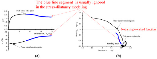
Figure 1. The turning hook of the stress−dilatancy curve corresponds to the main part of the loading process:(a) stress ratio versus axial strain curve and volumetric strain versus axial strain curve; (b) stress-dilatancy curve. (Data from Wu et al., 2021 [1], calcareous sand, confining pressure = 100 kPa).

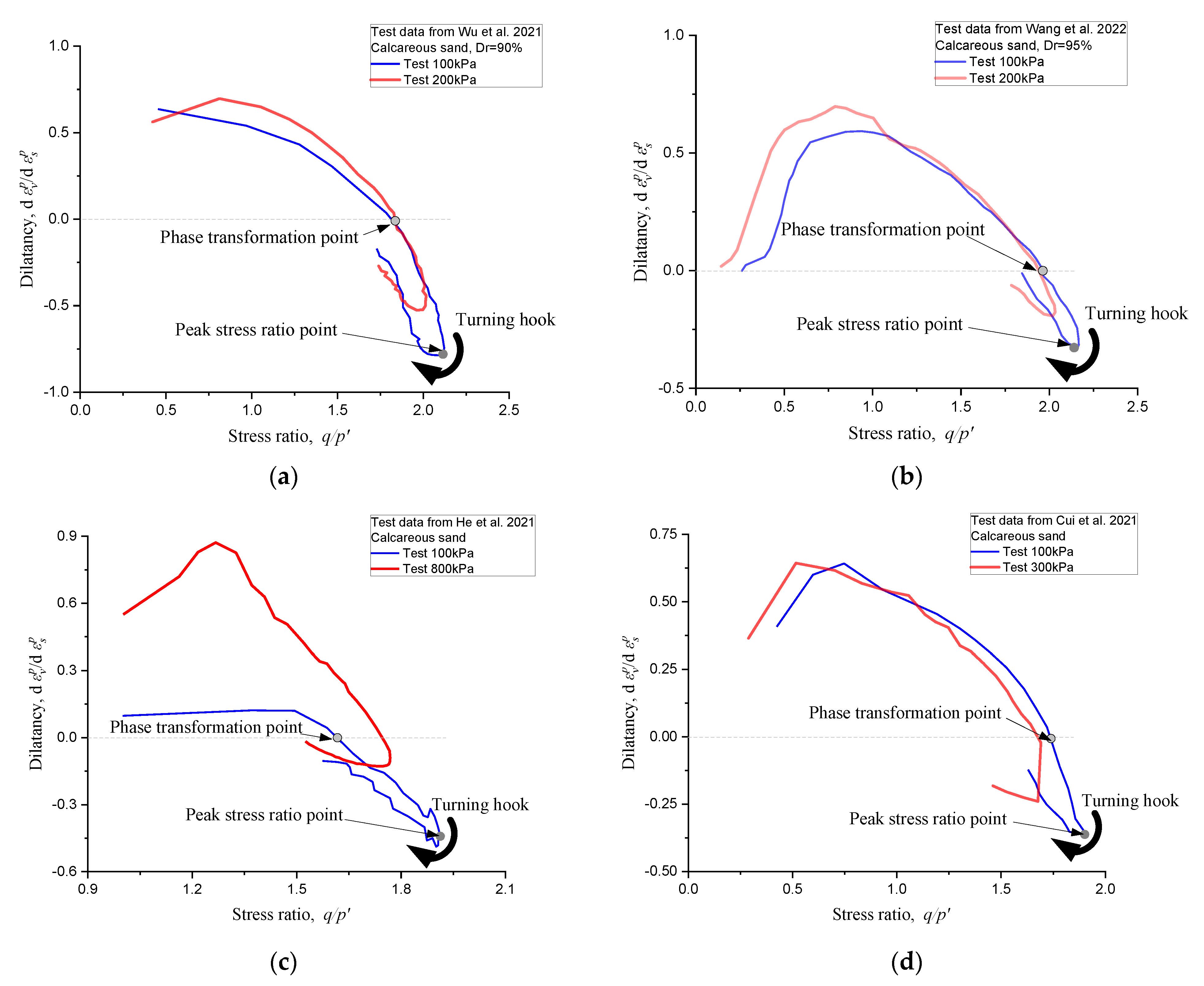
The above-mentioned turning hooks are shown by various triaxial tests. Figure 2 shows the turning hooks of five calcareous sands (Wu et al., 2021 [1], Wang et al., 2022 [2], He et al., 2021 [3], Cui et al., 2021 [4], Zhang & Luo 2020 [5]) and one MICP (microbially induced carbonate precipitation) stabilized calcareous sand (Cui et al., 2021 [4]).

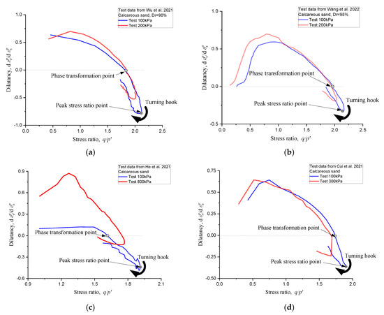
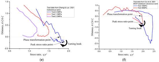
Figure 2. Turning hooks of stress−dilatancy curves of five crushable calcareous sands and one MICP-stabilized calcareous sand: (a) Wu et al., 2021 [1]; (b) Wang et al., 2022 [2]; (c) He et al., 2021 [3]; (d) Cui et al., 2021 [4]; (e) Zhang & Luo 2021 [5]; (f) Cui et al., 2021 [4].

However, the existing stress-dilatancy models usually ignore such turning hooks, i.e., the curve after the peak stress ratio point is not depicted. For instance, those models include classic soil models, such as Cam-Clay model (Roscoe&Burland 1968 [6]), Modified Cam-Clay model (Schofield& Wroth1968 [7]) and Rowe’s model (Rowe 1962 [8]); those models also include plastic models for non-crushable sands (Lu et al., 2021 [9], Gajo et al., 2019 [10], Yan & Li 2011 [11], Yu et al., 2007 [12]), models for crushable calcareous sands derived under the framework of thermodynamics (Collins & Hilder 2002 [13]; Collins & Muhunthan 2003 [14]; Collins et al., 2005 [15], Zhang et al., 2021 [16], Xiao et al., 2021 [17]), and models for crushable calcareous sand established by Zhang & Luo 2020 [5] and Wang et al., 2022 [2].

The difficulty in modeling the whole turning hook is that dilatancy is not a single-valued function of stress ratio (see Figure 1b), the turning hook around the peak stress ratio point). Thus, it is difficult to find a function that directly fits the stress-dilatancy relationship.

This paper presents a method to capture the turning hook of the stress-dilatancy curve, especially for the line segment after the peak stress ratio point. Based on the first law of thermodynamics, we related dilatancy to breakage energy which was mapped from the stress-energy plane to the strain-energy plane. Then we established a relationship between stress ratio and shear strain. Based on the above two works, our stress-dilatancy model is conveniently established to capture the entire turning hook. We performed triaxial tests on colloidal-silica-stabilized calcareous sand to verify our model and compare our model to four existing stress-dilatancy models. Our model is also verified by MICP-stabilized calcareous sand and three types of calcareous sands in the literatures.

2. Stress-DilatancyModel

2.1. Model Establishment

Based on the first law of thermodynamics, we assume that the plastic part of external work done on the boundaries of the sand sample is equal to the sum of dissipation and breakage energy, as shown in Equation (1).

$$W=\mathsf{\Phi }+E_B$$

(1)

where $W$ is the plastic work on the boundaries, $\mathsf{\Phi }$ is the dissipation, and $E_B$ is the breakage energy. Here we ignore elasticity strain energy, as Wan & Guo (1999) [18], Li &Dafalias (2000) [19], and Hanley et al. (2018) [20] treated the sand specimens, which means ε_v ≈ ${\epsilon }_v^p$ and ε_s ≈ ${\epsilon }_s^p$, where ε_v, ${\epsilon }_v^p$, ε_s and ${\epsilon }_s^p$ are volumetric strain, plastic volumetric strain, shear strain and plastic shear strain, respectively. By differentiating Equation (1), we have

$$\dot{W}=\dot{\mathsf{\Phi }}+{\dot{E}}_B$$

(2)

where $\dot{W}$, $\dot{\mathsf{\Phi }}$ and ${\dot{E}}_B$ are the rates of $W$, $\mathsf{\Phi }$, and $E_B$, respectively. ${\dot{E}}_B$ represents the rate of breakage energy and should be no less than zero. The boundary work rate $\dot{W}$ can be expressed in triaxial variables using

$$\dot{W}=p^{\prime }\mathrm{d}{\epsilon }_v^p+q\mathrm{d}{\epsilon }_s^p$$

(3)

where $p^{\prime }$ is the mean effective stress, $q$ is the triaxial shear stress, $\mathrm{d}{\epsilon }_v^p$ is plastic volumetric strain increment, and $\mathrm{d}{\epsilon }_s^p$ is plastic shear strain increment. We assume the dissipation rate has the form of Cam Clay Model

$$\dot{\mathsf{\Phi }}=p\cdot M\cdot \mathrm{d}{\epsilon }_s^p$$

(4)

where $M$ is the stress ratio at the critical state. Here we mainly consider the breakage during triaxial shearing, so the form of breakage energy rateis assumed as shown in Equation (5).

$${\dot{E}}_B=\frac{\mathrm{d}{E}_B}{\mathrm{d}{\epsilon }_s^p}\mathrm{d}{\epsilon }_s^p$$

(5)

Substituting Equations (3)–(5) into Equation (2), we have the following equation.

$$\frac{\mathrm{d}{\epsilon }_v^p}{\mathrm{d}{\epsilon }_s^p}=M-\eta +\frac{1}{p^{\prime }}\frac{\mathrm{d}{E}_B}{\mathrm{d}{\epsilon }_s^p}$$

(6)

where $\eta$ is the stress ratio and $\eta =q/p^{\prime }$.

Next, we need to get the form of breakage-energy related variable $\mathrm{d}{E}_B/\mathrm{d}{\epsilon }_s^p$ in Equation (6). Though we can get the curves of $\mathrm{d}{E}_B/\mathrm{d}{\epsilon }_s^p$ versus stress ratio $\eta$ from triaxial tests, it is difficult to give an analytical expression for $\mathrm{d}{E}_B/\mathrm{d}{\epsilon }_s^p$ in terms of $\eta$ directly, since $\mathrm{d}{E}_B/\mathrm{d}{\epsilon }_s^p$ is not a single-valued function of stress ratio $\eta$ (see Figure 1b). So we map breakage-energy related variable from the stress-energy plane to the strain-energy plane, i.e., we map $\mathrm{d}{E}_B/\mathrm{d}{\epsilon }_s^p$ from the $\mathrm{d}{E}_B/\mathrm{d}{\epsilon }_s^p$ vs. $\eta$ plane to the $\mathrm{d}{E}_B/\mathrm{d}{\epsilon }_s^p$ vs. ${\epsilon }_s^p$ plane. Then it is easier to get the form of $\mathrm{d}{E}_B/\mathrm{d}{\epsilon }_s^p$ expressed in terms of shear strain ${\epsilon }_s^p$, since the derivative of breakage energy $\mathrm{d}{E}_B/\mathrm{d}{\epsilon }_s^p$ is a single-valued function of ${\epsilon }_s^p$.

We use the normal-distribution-type function to fit the derivative of breakage energy on the strain-energy plane, as shown in Equation (7).

$$\frac{\mathrm{d}{E}_B}{\mathrm{d}{\epsilon }_s^p}=\frac{p^{\prime }}{\sqrt{2\pi }{C}_1}\exp \left(\frac{-{\left({\epsilon }_s^p-C_2\right)}^2}{2B_1^2}\right)+p^{\prime }{C}_3-p^{\prime }M+p^{\prime }\eta$$

(7)

where $B_1^{}$, $C_1$, $C_2$ and $C_3$ are parameters, respectively. Substituting Equation (7) into Equation (6) yields

$$\frac{\mathrm{d}{\epsilon }_v^p}{\mathrm{d}{\epsilon }_s^p}=\frac{1}{\sqrt{2\pi }{C}_1}\exp \left(\frac{-{\left({\epsilon }_s^p-C_2\right)}^2}{2B_1^2}\right)+C_3$$

(8)

To fulfill the requirement of critical state, i.e., when ${\epsilon }_s^p\to \infty$, we have $\mathrm{d}{\epsilon }_v^p/\mathrm{d}{\epsilon }_s^p\to 0$, so replacing $C_3$ in Equation (8) with $C_3\exp \left(-{\epsilon }_s^p\right)$ yields Equation (9).

$$\frac{\mathrm{d}{\epsilon }_v^p}{\mathrm{d}{\epsilon }_s^p}=\frac{1}{\sqrt{2\pi }{C}_1}\exp \left(\frac{-{\left({\epsilon }_s^p-C_2\right)}^2}{2B_1^2}\right)+C_3\exp \left(-{\epsilon }_s^p\right)$$

(9)

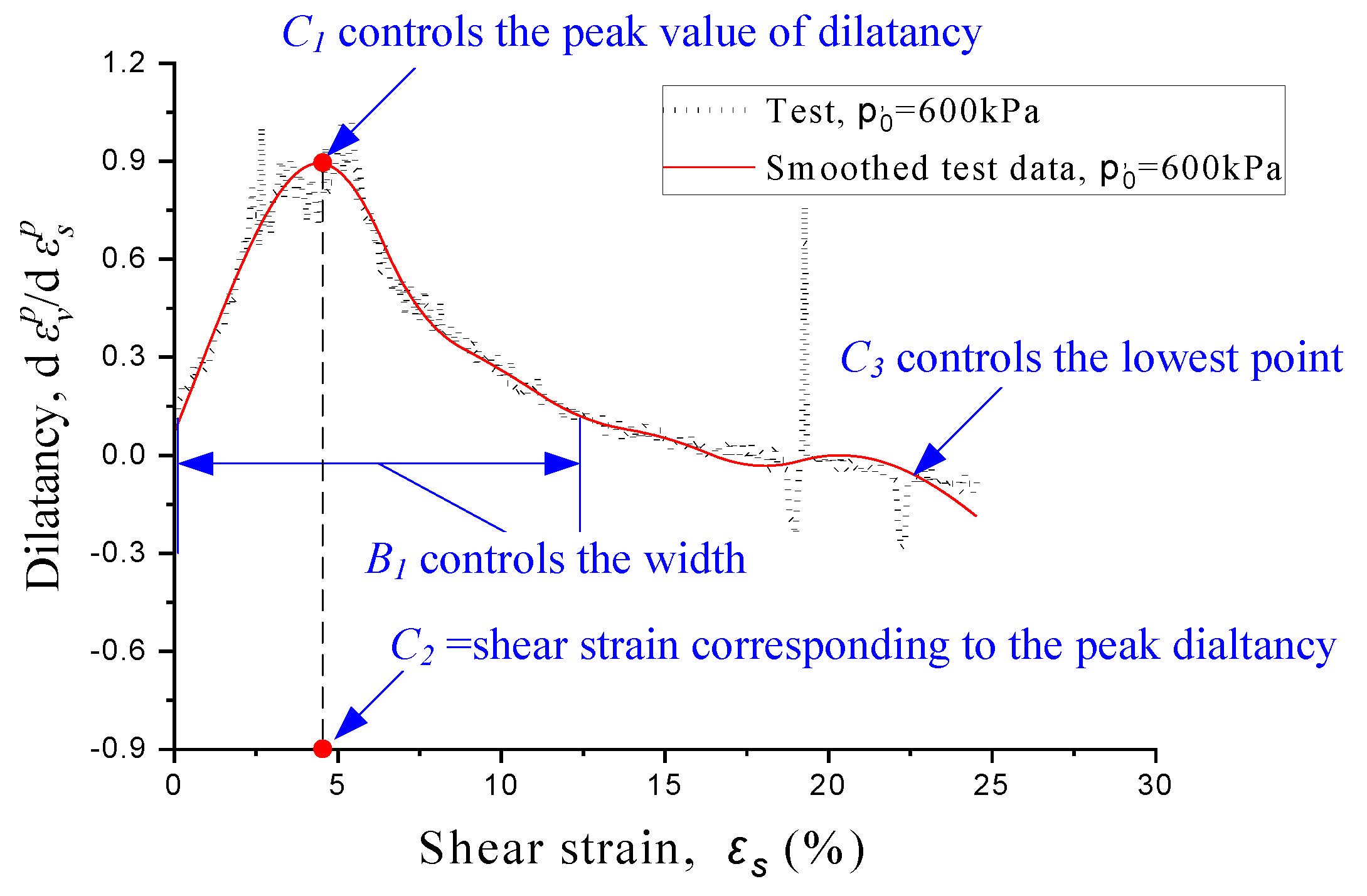
In Figure 3, we show the effect of these parameters on the curve of dilatancy versus shear-strain: $B_1^{}$ controls the horizontal width of the curve, $C_1$ controls the peak dilatancy, $C_2$ is equal to the shear strain corresponding to the peak dilatancy, and $C_3$ controls the minimum value of the curve.

Figure 3. Smoothing test data for dilatancy fitting on the strain−dilatancy plane.

We smooth the curve of dilatancy versus shear strain for curve fitting, as shown by the red line in Figure 3, since the test curve (see the dotted line in Figure 3) has too many burrs which make our curve fitting difficult. These burrs are caused by taking the derivative of the test data of the volumetric strain. We smooth the test data in the following steps: (1) for the test data, we take the volumetric strain every 30 points, then get the spline-interpolated curve of volumetric-strain versus shear-strain; (2) by the first-order differentiation of the spline-interpolated volumetric-strain with respect to shear-strain, we get the smoothed curve of dilatancy versus shear-strain (see the red line in Figure 3). Note that our parameter calibration is based on the smoothed strain-dilatancy curve.

Traditionally, stress-dilatancy model is defined on the plane of dilatancy vs. stress ratio, so we need to convert Equation (9) from the strain-dilatancy plane to the stress-dilatancy plane. Here we establish the relationship between the stress ratio and the shear strain to complete this conversion. This relationship is shown in Equation (10).

$$\frac{q}{p}=\frac{\beta {\left(\frac{e_c}{e}\right)}^{m}M{\epsilon }_s^p}{{\left(\frac{e_c}{e}\right)}^{m}M+\beta {\epsilon }_s^p}$$

(10)

where $m$ and $\beta$ are parameters, $e$ is the void ratio and $e_c$ is the void ratio at the critical state. At the critical state, for the left of Equation (10) we have $q/p\to M$, while for the right side, when ${\epsilon }_s^p\to \infty$ we have $e\to e_c$ and $\beta {\left(e_c/e\right)}^{m}M{\epsilon }_s^p/\left. [{\left(e_c/e\right)}^{m}M+\beta {\epsilon }_s^p\right]\to M$. Therefore, at the critical state both sides of Equation (10) are equal to $M$, respectively, so that Equation (10) fulfills the requirement of critical state.

Equation (10) is rewritten to express ${\epsilon }_s^p$ as a function of $q/p$, as shown in Equation (11).

$${\epsilon }_s^p=\frac{\frac{q}{p}{\left(\frac{e_c}{e}\right)}^{m}M}{\beta {\left(\frac{e_c}{e}\right)}^{m}M-\beta \frac{q}{p}}$$

(11)

Substituting Equation (11) into Equation (9) yields the flow rule on the stress-dilatancy plane, as shown in Equation (5).

$$\frac{\mathrm{d}{\epsilon }_v^p}{\mathrm{d}{\epsilon }_s^p}=\frac{1}{\sqrt{2\pi }{C}_1}\exp \left(\frac{-1}{2B_1^2}{\left(\frac{\frac{q}{p}{\left(\frac{e_c}{e}\right)}^{m}M}{\beta {\left(\frac{e_c}{e}\right)}^{m}M-\beta \frac{q}{p}}-C_2\right)}^2\right)+C_3\exp \left(-\frac{\frac{q}{p}{\left(\frac{e_c}{e}\right)}^{m}M}{\beta {\left(\frac{e_c}{e}\right)}^{m}M-\beta \frac{q}{p}}\right)$$

(12)

2.2. Effects of Parameters on Dilatancy

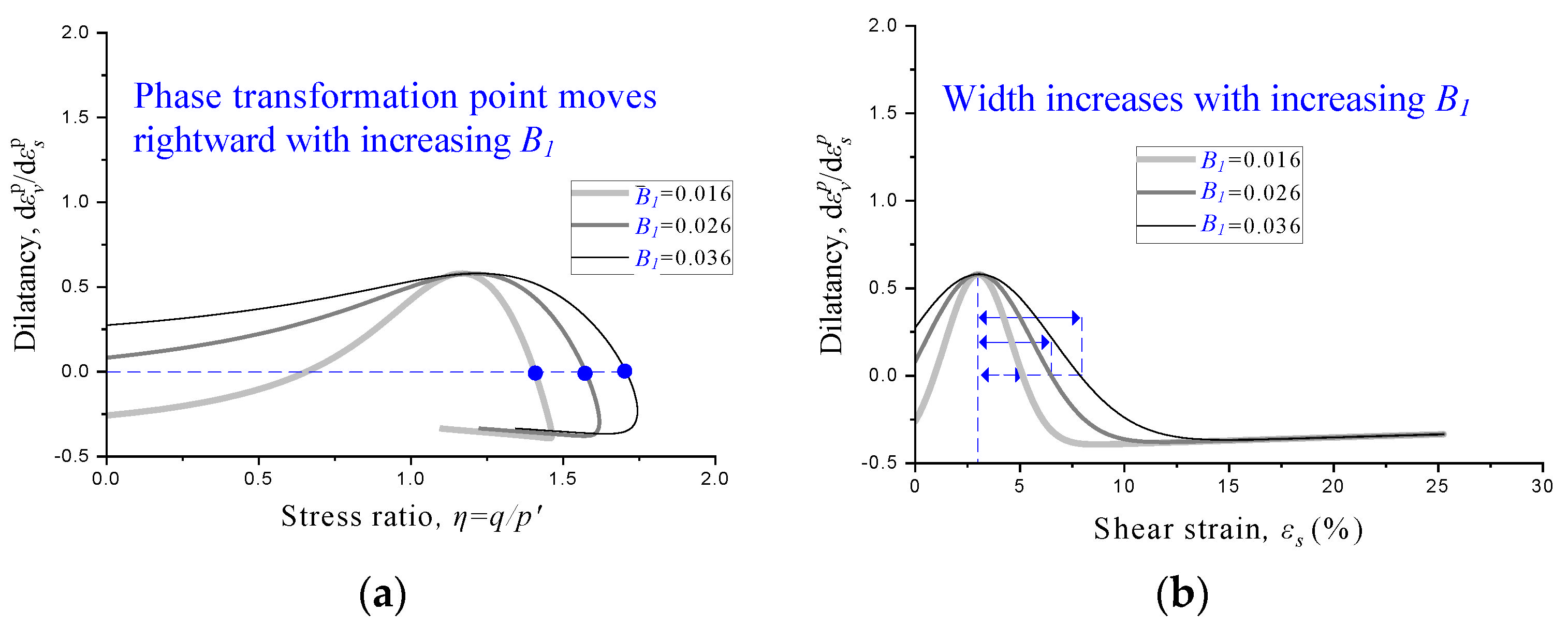
Here we show the effect of $B_1^{}$, $C_1$, $C_2$ and $C_3$ on the dilatancy $\mathrm{d}{\epsilon }_v^p/\mathrm{d}{\epsilon }_s^p$. Figure 4 shows that as $B_1^{}$ increases, the horizontal width of the curve increases on the strain-dilatancy plane (see Figure 4a), while the phase transformation point (namely the peak volumetric strain point and $\mathrm{d}{\epsilon }_v^p/\mathrm{d}{\epsilon }_s^p$ = 0) moves rightward on the stress-dilatancy plane (see Figure 4b).

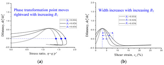
Figure 4. Effect of B₁ on dilatancy: (a) flow rule defined on the plane of dilatancy versus shear strain, and (b) flow rule defined on the stres−dilatancy plane.

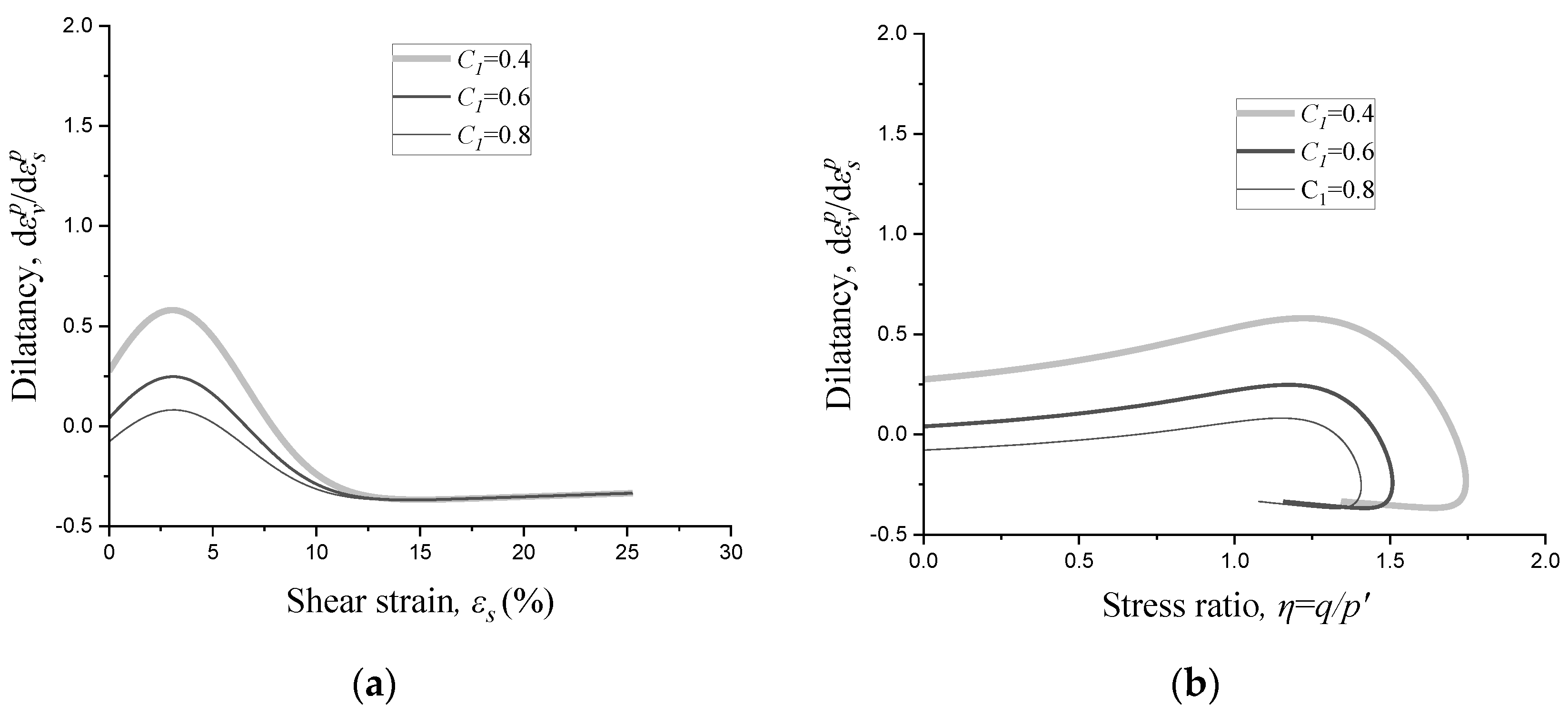
Figure 5 shows that $C_1$ controls the peak dilatancy. As $C_1$ increases, the peak dilatancy decreases onboth the strain−dilatancy plane (see Figure 5a) and the stress−dilatancy plane (see Figure 5b).

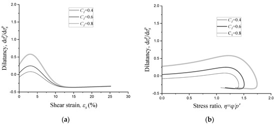
Figure 5. Effect of C₁ on dilatancy: (a) flow rule defined on the plane of dilatancy versus shear strain, and (b) flow rule defined on the stress−dilatancy plane.

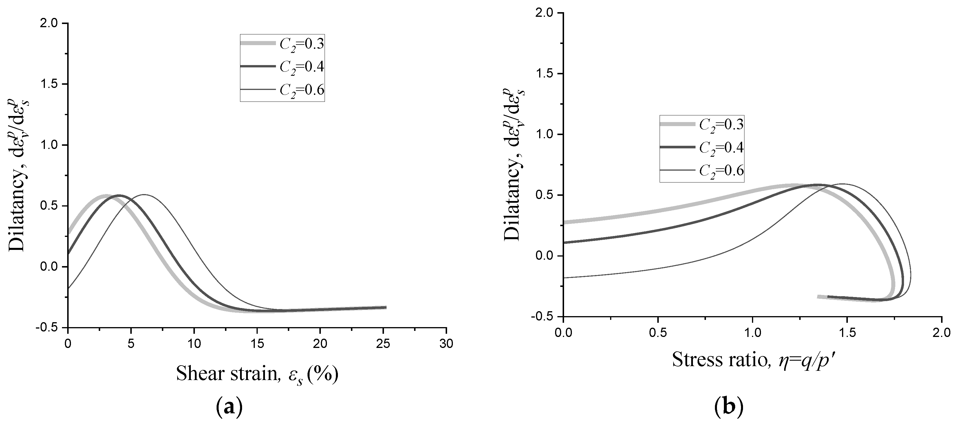
Figure 6 shows that $C_2$ controls the shear strain corresponding to the peakdilatancy. As $C_2$ increases, the phase transformation points and the curves move rightward onboth the strain-dilatancy plane (see Figure 6a) and the stress-dilatancy plane (see Figure 6b).

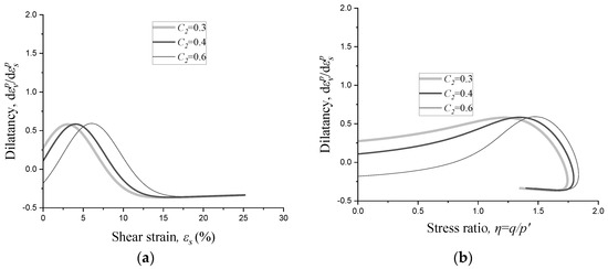
Figure 6. Effect of C₂ on dilatancy: (a) flow rule defined on the plane of dilatancy versus shear strain, and (b) flow rule defined on the stress−dilatancy plane.

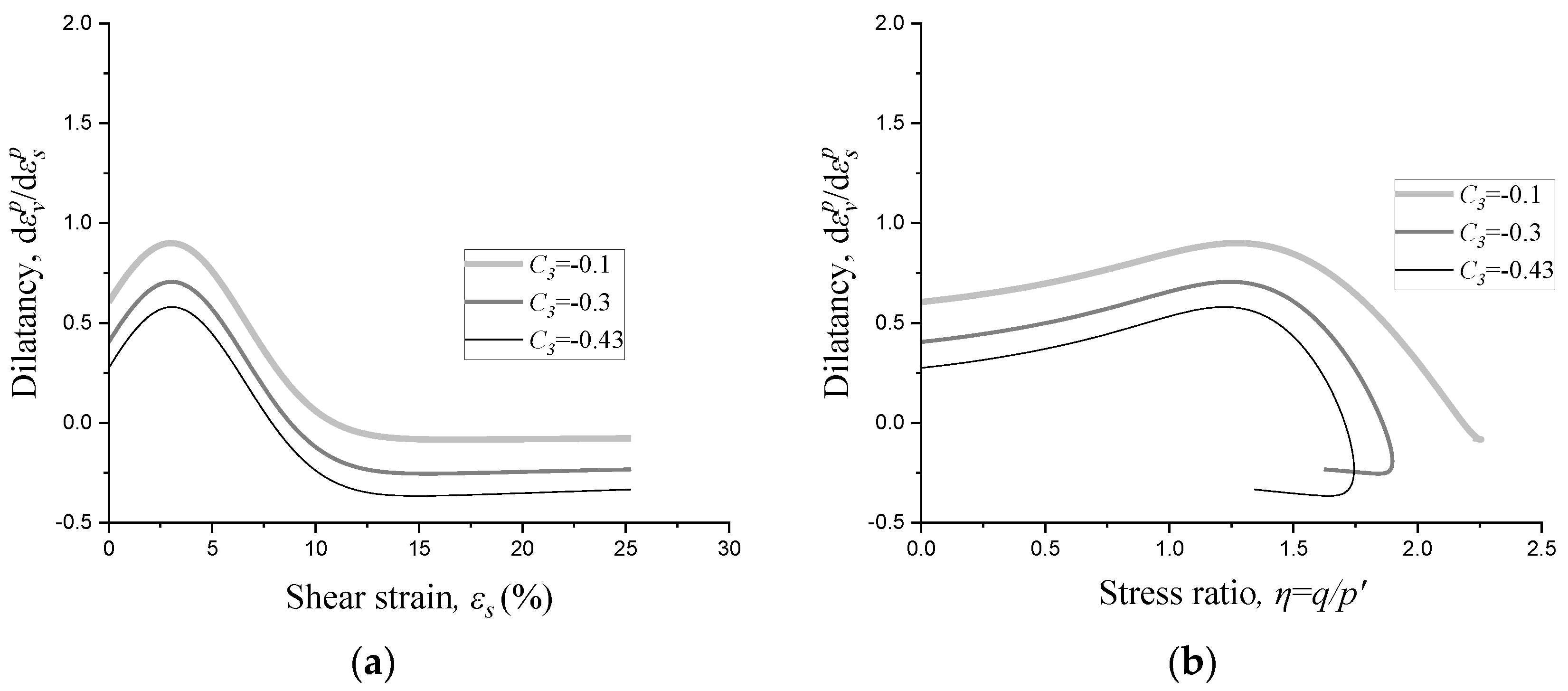
Figure 7 shows that $C_3$ controls the lowest value of dilatancy. As $C_3$ increases, the curves move upwardonboth the strain-dilatancy plane (see Figure 7a) and the stress−dilatancy plane (see Figure 7b).

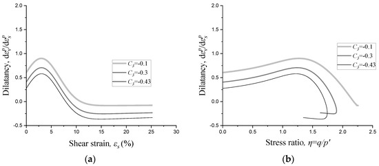
Figure 7. Effect of C₃ on dilatancy: (a) flow rule defined on the plane of dilatancy versus shear strain, and (b) flow rule defined on the stress−dilatancy plane.

3. Model Verification by Colloidal-Silica-Stabilized Calcareous Sand

We performed triaxial tests on calcareous sand stabilized by nanowire-dispersed colloidal silica. Then we use the test data to verify our stress-dilatancy model.

3.1. Experimental Materials

The marine calcareous sand used was from the Philippines. Index properties of the sand are listed in Table 1.

Table 1. Properties of sand sample.

Specific Gravity, Gs	Max. Dry Density (kg/m3)	Min. Dry Density (kg/m3)	Relative Density	Coefficient of Uniformity, Cu	Coefficient of Curvature, Cc
2.79	1370	1190	0.516	1.9	1.09

Colloidal silica can seep rapidly and meet the requirement of long-distance transportationthrough sand due to its low viscosity, then nano-silica particles in the colloidal silica agglomerate to form gel to cement sand particles. Extensive experiments have been performed to study the properties of sand stabilized by colloidal silica [21,22,23,24,25,26,27,28,29]. The colloidal silica was provided by Qingdao Maike Silica Gel Dessicant Co., Ltd., Qingdao, China, and the concentration used was 20% by weight. For colloidal silica, silica nano-particles are suspended and repel each other under an alkaline environment, with diameter distributions of 10–20 nm. The physical properties of the colloidal silica are shown in Table 2.

Table 2. Physical properties of the colloidal silica.

SiO2 (%)	pH	Density (g/cm3)	Viscosity (Pa.s)	Average Particle Size (nm)
20%	8.5~10.0	1.12~1.14	5.0 × 10−3	10~20

Fiber-dispersed colloidal silica can enhance the strength of stabilized sand [30,31]. The silicon carbide (SiC) nanowires used in the testswere produced by Nanjing Xianfeng Nano Material Technology Co., Ltd., Nanjing, China.The content of SiC nanowiresis 0.02% by weight of colloidal silica. The physical properties of SiC nanowires are shown in Table 3.

Table 3. Properties of SiC nanowires.

Diameter (nm)	Length (μm)	Density (g/cm3)	Purity (%)
100–600	50–100	3.21	98

3.2. Specimen Preparation and Testing Apparatus

The specimens of stabilized calcareous sand were formed as the following steps: first, the pH of the colloidal silica was adjusted to 5.0–5.5 by adding acetic acid, then the colloidal silica was stirred with SiC nanowires for 30 min by a magnetically driven bar (see Figure 8a); secondly, SiC nanowires were further dispersed by ultrasonic dispersion for 60 min (see Figure 8b); finally, by using a peristaltic pump, SiC-nanowire-dispersed colloidal-silica was slowly injected into the sand from the bottom of a cylindrical mold (see Figure 8c). Then the liquid colloidal silica was gradually transformed into solid silica gel, and the SiC nanowires dispersed in the silica gel served as reinforcing fibers. This SiC-nanowire-reinforced silica-gel could bond sand particles, thereby stabilizing sand specimens. The stabilized specimens were cured for 3 days before testing.

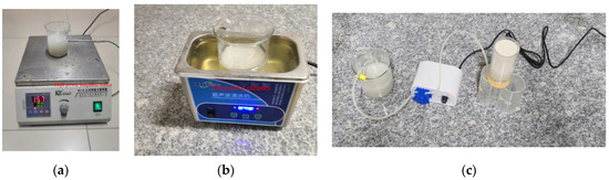
Figure 8. Specimen preparation: (a) magnetically stirred mixture of SiC nanowires and colloidal silica, (b) ultrasonic dispersion of SiC nanowires in colloidal silica, and (c) the SiC-nanowire-dispersed colloidal-silica seeped through sand.

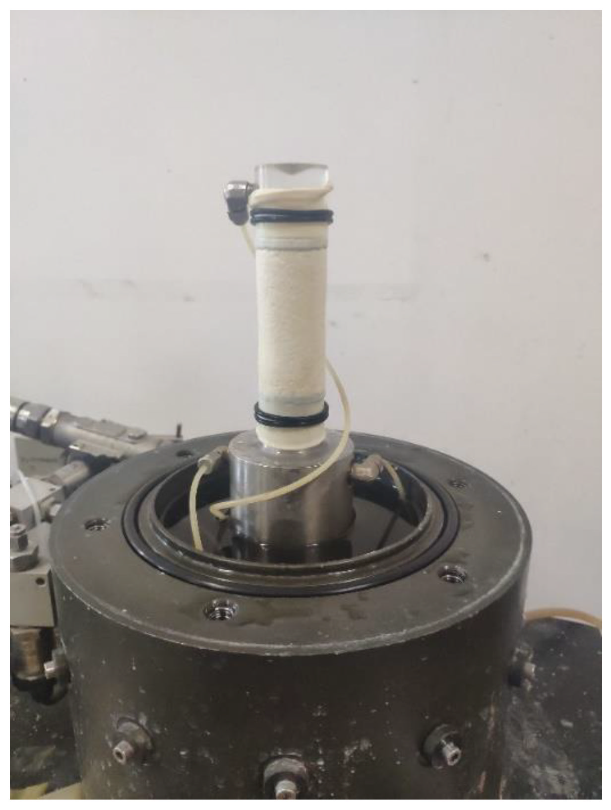
AGDS advanced triaxial system (see Figure 9) was used to carry out drained triaxial compression tests on specimens. The diameter and height of the test specimen were 38 mm and 76 mm, respectively.

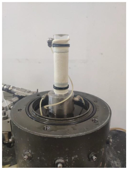
Figure 9. Specimen for drained triaxial compression test.

3.3. Experimental Plan

For stabilized specimens, the initial mean effective stresses in drained triaxial tests were 100 kPa, 200 kPa and 600 kPa. At the initial mean effective stresses of 100 kPa, 200 kPa and 600 kPa, the initial void ratios were 0.731, 0.701, and 0.652, respectively. All the specimens were fully saturated. During each triaxial test, the confining pressure (horizontal stress) is set equal to the initial mean effective stress. To illustrate the particle breakage, unstabilized calcareous sands were sieved after triaxial testing to show the changes in particle size distribution.

3.4. Testing Results

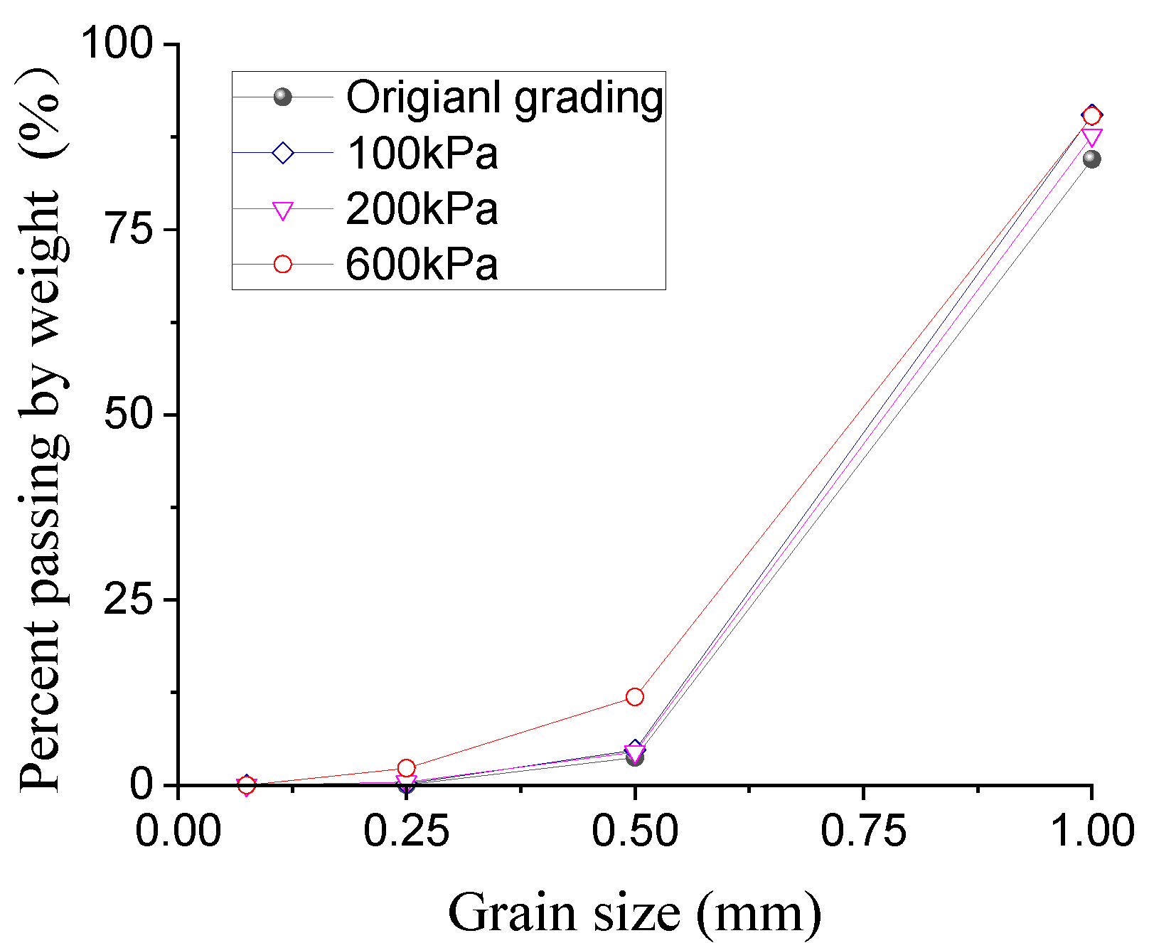
To illustrate the occurrence of particle breakage, for unstabilized calcareous sand, Figure 10 shows grain size distribution (GSD) curves before and after the triaxial tests. Apparently, the amount of breakage increases as the initial mean effective stress increases from 100 kPa to 600 kPa.

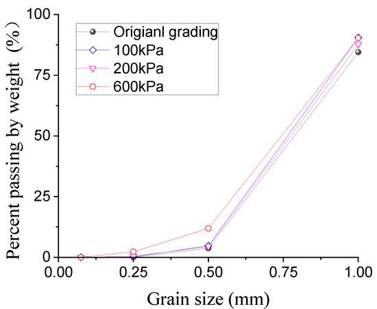
Figure 10. Grain size distribution of unstabilized calcareous sand after triaxial tests.

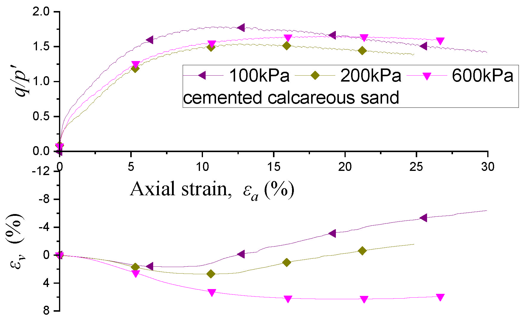
Figure 11 shows stress ratios and volumetric strains of stabilized calcareous sand under different initial mean effective stresses. Here $q/p^{\prime }$ denotes the stress ratio, and $q$ and $p^{\prime }$ are the shear stress and the mean effective stress, respectively. For the volumetric strain versus axial strain curves, since volumetric strain is defined as positive when contraction occurs, the specimens contract first then dilate under low initial mean effective stresses (100 kPa and 200 kPa), while under relatively high initial mean effective stress (600 kPa) the specimen mainly exhibits contraction.

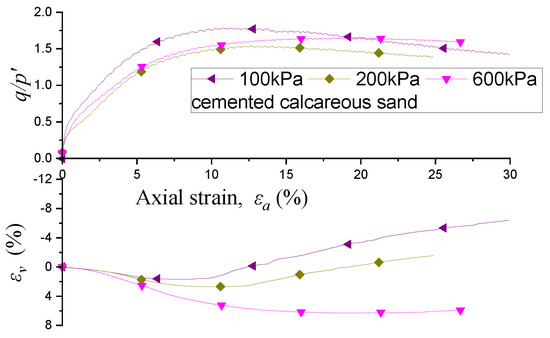
Figure 11. Stress ratio and volumetric strain behaviors of stabilized calcareous sand.

3.5. Parameter Determination

For the parameters used in Equation (10), $M$ is the stress ratio at the critical state, $\beta$ is the initial slope of the curve of stress-ratio versus shear-strain, and $m$ affects the peak value of stress ratio and is determined by fitting the test curve of stress-ratio versus shear-strain. Finally, these three parameters,$M$, $\beta$, and $m$, are, respectively, determined as the average value of tests with different initial mean effective stresses. Another variable $e_c$ is the void ratio at the critical state and we express it as a function of initial mean effective stress, as shown in Equation (13).

$$e_c=e_{\Gamma }^0-{\lambda }_c^0\mathrm{In}\left({p^{\prime }}_0\right)$$

(13)

where $e_{\Gamma }^0$ and ${\lambda }_c^0$ are curve fitting parameters and are determined as 2.68 and 0.16, respectively.

For parameters in the flow rule on the strain-dilatancy plane, we determine the values of $B_1^{}$, $C_1$, $C_2$ and $C_3$ in the following steps:

Step 1: For $C_2$, let ${\epsilon }_s^{d\max }$ be the shear stress corresponding to the peak dilatancy, and we set $C_2$ = ${\epsilon }_s^{d\max }$. Then we take the average value of $C_2$ from tests with different initial mean effective stresses.

Step 2: Based on Equation (9), $C_3$ controls the minimum value of dilatancy and is determined by fitting the test curve of dilatancy versus shear strain; we use the least square method to fit $C_3$ as a function of initial mean effective stress ${p^{\prime }}_0$, as shown in Equation (14).

$$C_3=C_a+C_b\mathrm{In}\left({p^{\prime }}_0\right)$$

(14)

where $C_a$ and $C_b$ are the parameters of least-squares fitting and are determined as −3.52 and 0.26, respectively.

Step 3: $C_1$ controls the peak dilatancy which is denoted as $d_{\max }$. Then Substituting $C_2$ = ${\epsilon }_s^{d\max }$ (obtained in Step 1), $C_3$ (obtained in Step 2), ${\epsilon }_s^p$ = ${\epsilon }_s^{d\max }$ (obtained from test), and $C_1$ = $d_{\max }$ (obtained from test) into Equation (9) yields Equation (15) for calculating $C_1$. We take the average value of $C_1$ from tests with different initial mean effective stresses.

$$C_1=\frac{1}{\sqrt{2\pi }\left(d_{\max }-C_3\exp \left(-{\epsilon }_s^{d\max }\right)\right)}$$

(15)

Step 4: $B_1^{}$ is determined by the transformation point (namely the peak volumetric strain point where $\mathrm{d}{\epsilon }_v^p/\mathrm{d}{\epsilon }_s^p$ = 0). Let ${\epsilon }_s^{V\max }$ be the shear strain corresponding to the transformation point, then substituting ${\epsilon }_s^p$ = ${\epsilon }_s^{V\max }$, $\mathrm{d}{\epsilon }_v^p/\mathrm{d}{\epsilon }_s^p$ = 0, $C_1$ (obtained in Step 3), $C_2$ (obtained in Step 1) and $C_3$ (obtained in Step 2) into Equation (9) yields Equation (16) for calculating $B_1^{}$. We take the average value of $B_1^{}$ from tests with different initial mean effective stresses.

$$B_1^{}=\sqrt{-\frac{{\left({\epsilon }_s^{V\max }-C_2\right)}^2}{2\mathrm{In}\left(-\sqrt{2\pi }{C}_1{C}_3\exp \left(-{\epsilon }_s^p\right)\right)}}$$

(16)

Parameters used for stress-dilatancysimulation are listed in Table 4.

Table 4. Parameters for prediction of calcareous sand under breakage and cementation failure.

$\mathit{M}$	$\mathit{\beta }$	$\mathit{m}$	${\mathit{e}}_{\mathit{\Gamma }}^0$	${\mathit{\lambda }}_{\mathit{c}}^0$	${\mathit{B}}_1$	${\mathit{C}}_1$	${\mathit{C}}_2$	${\mathit{C}}_3$
								${\mathit{C}}_{\mathit{a}}$	${\mathit{C}}_{\mathit{b}}$
1.49	120	2.9	2.68	0.16	0.036	0.42	0.039	−3.52	0.26

3.6. Simulation of Stress-Dilatancy Relationship

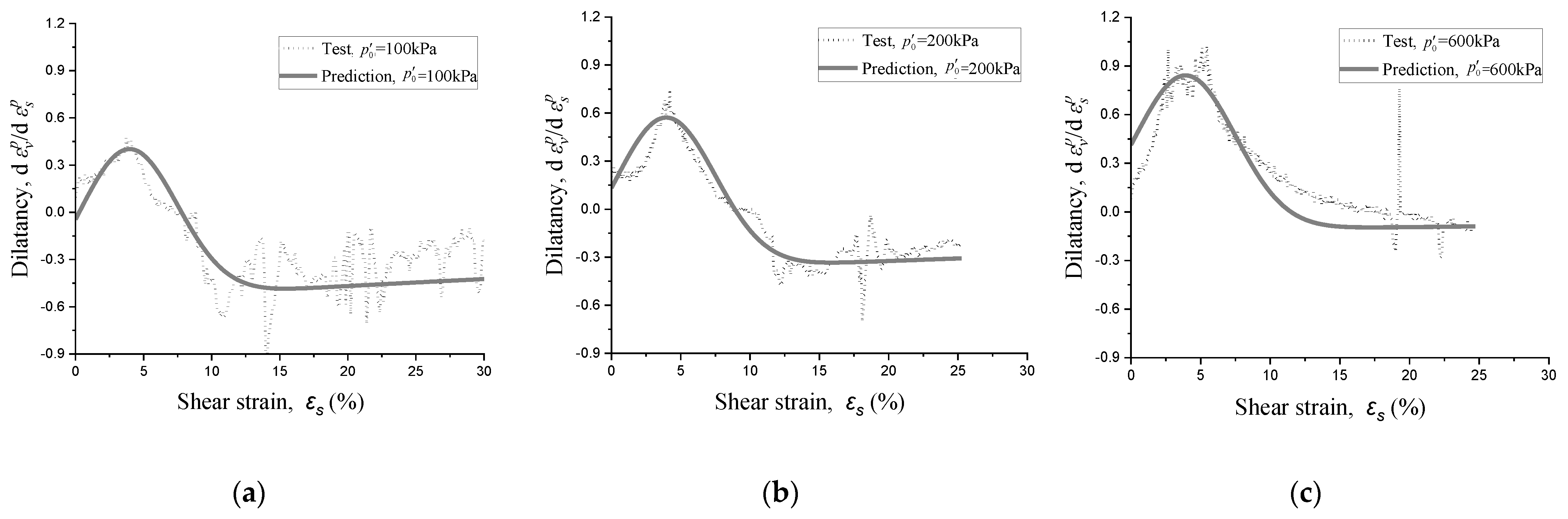
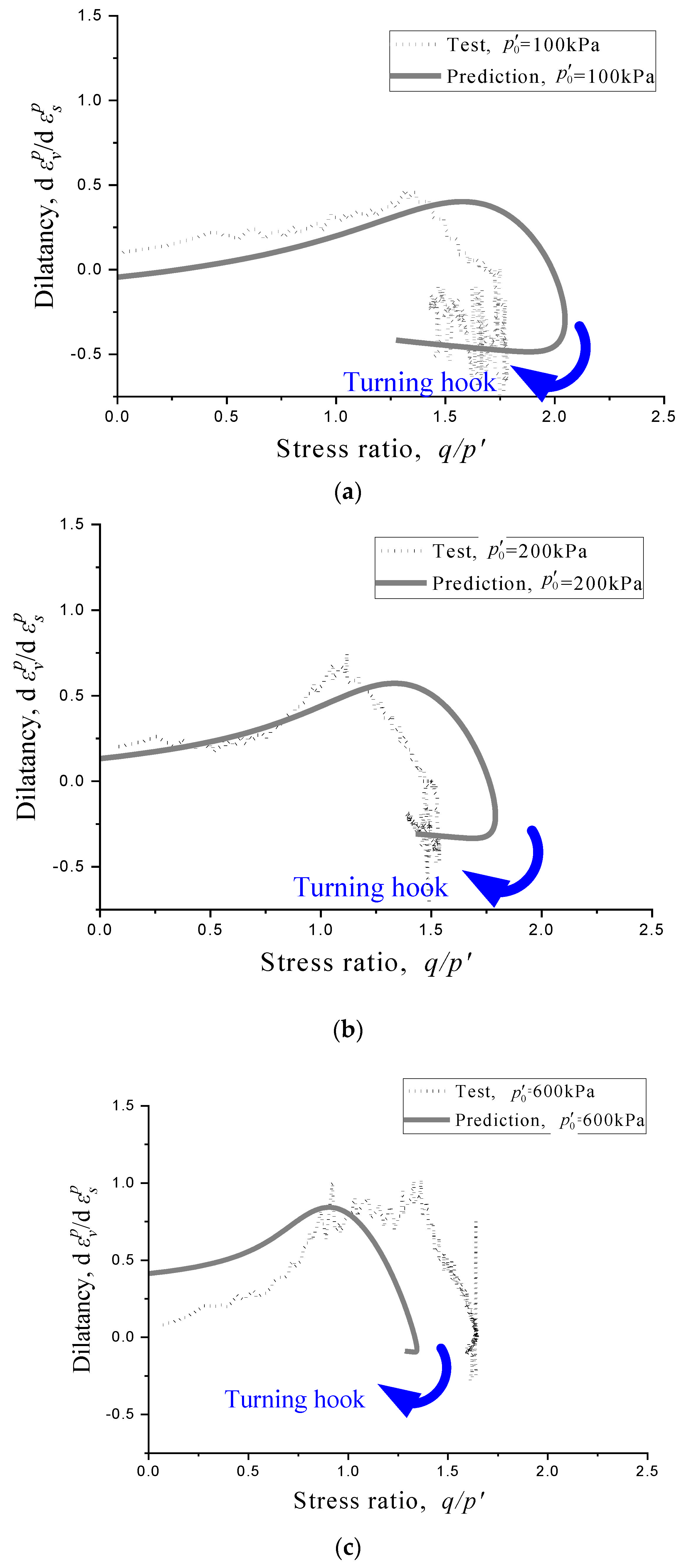
Our prediction of dilatancy is in good agreement with the test curves on the plane of dilatancy versus shear-strain, as shown in Figure 12. When the dilatancy in Figure 12 is converted to the stress-dilatancy plane, we can obtain the stress-dilatancy relationship (see Figure 13). Here we use Equations (9) and (10) to plot the stress-dilatancy curve, i.e., we use Equations (9) and (10) to calculate dilatancy $\mathrm{d}{\epsilon }_v^p/\mathrm{d}{\epsilon }_s^p$ and stress ratio $q/p$, respectively, then use the shear strain to relate the corresponding dilatancy $\mathrm{d}{\epsilon }_v^p/\mathrm{d}{\epsilon }_s^p$ and stress ratio $q/p$. Our stress-dilatancy model shows the characteristics of the test data, i.e., our model can capture the turing hook of stress-dilatancy curve, especially the line segment after the peak stress ratio (see Figure 13). We established Equation (10) for relating the stress ratio q/p to the shear strain. Figure 13 shows that, this yield-fuction-like equation overpredicts the stress ratio q/p at p₀ = 100 kPa and 200 kPa, while it underpredicts the stress ratio at p₀ = 600 kPa. So, a more precise yield function needs to be established to relate the stress ratio to the shear strain better than Equation (10).

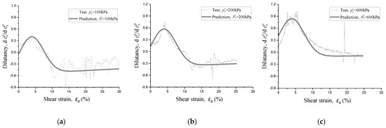
Figure 12. Prediction of dilatancy on the plane of dilatancy versus shear strain: (a) ${p^{\prime }}_0$ = 100 kPa, (b) ${p^{\prime }}_0$ = 200 kPa, and (c) ${p^{\prime }}_0$ = 600 kPa.

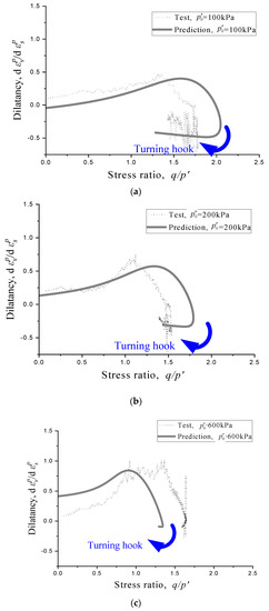
Figure 13. Prediction of the turning hooks of the stress−dilatancy curves: (a) ${p^{\prime }}_0$ = 100 kPa, (b) ${p^{\prime }}_0$ = 200 kPa, and (c) ${p^{\prime }}_0$ = 600 kPa.

4. Comparison with Four Existing Models

4.1. Introduction of the Four Existing Stress-Dilatancy Models

Here we compare our model with four existing stress-dilatancy models, i.e., the original Cam-Clay model, the modified Cam-Clay model, Rowe’s model, and Li and Daflias’s model. The expressions of these four models are as follows. The tests providing stress-dilatancy relationships are shown in Section 3.

Schofield and Wroth [6] presented the stress-dilatancy model in the well-known original Cam Clay model:

$$\frac{\mathrm{d}{\epsilon }_v^p}{\mathrm{d}{\epsilon }_s^p}=M-\eta$$

(17)

where $\mathrm{d}{\epsilon }_v^p$ is the plastic volumetric strain increment, $\mathrm{d}{\epsilon }_s^p$ is the plastic shear strain increment, $M$ is the ratio of $q/p^{\prime }$ at critical state, $\eta$ is the stress ratio and $\eta =q/p^{\prime }$.

Roscoe and Burland [7] presented the stress-dilatancy model in the well-known Modified Cam Clay model:

$$\frac{\mathrm{d}{\epsilon }_v^p}{\mathrm{d}{\epsilon }_s^p}=\frac{M^2-{\eta }^2}{2\eta }$$

(18)

Rowe’s stress-dilatancy model [8]:

$$\frac{\mathrm{d}{\epsilon }_v^p}{\mathrm{d}{\epsilon }_s^p}=\frac{9\left(M-\eta \right)}{9+3M-2M\eta }$$

(19)

Li and Daflias’sstress-dilatancy model [19]:

$$\frac{\mathrm{d}{\epsilon }_v^p}{\mathrm{d}{\epsilon }_s^p}=\frac{d_0}{M}\left. [M\exp \left(m\psi \right)-\eta \right]$$

(20)

where $d_0$ and $m$ are two positive parameters, $\psi$ is the state variable and is defined as follows:

$$\psi =e-e_c$$

(21)

where $e$ is the void ratio and $e_c$ is the void ratio at the critical state.

4.2. Parameter Determination for the Four Existing Stress-Dilatancy Models

Here we illustrate how to determine the values of the parameters and variables during the integrations of Equations (17)–(20). All the parameters and variables on the right sides of Equations (17)–(20) are determined by test data. $M$ is obtained from the test data at the critical state, i.e., $M$ is set equal to the stress ratio $\eta$ at the final stable state (namely the critical state). During each numerical integration step, the stress ratio $\eta$ from the test data is substituted into Equations (17)–(20), respectively.

In addition, we need to determine the values of $\psi$, $d_0$ and $m$ in Equation (20). First, the state variable $\psi$ is determined by the void ratio $e$ and the critical void ratio $e_c$, as shown in Equation (21). During each numerical integration step, the void ratio $e$ from the test data is substituted into Equation (21), and $e_c$ is set equal to the void ratio at the critical state.

Secondly, for $d_0$, when we substituted different values of $d_0$ into Equation (20) for integration to obtain the volumetric strain, we found that $d_0$ can only adjust the peak value of the volumetric strain, but it can not adjust the shear strain at which the peak volumetric strain occurs. So, no matter what value $d_0$ takes, the prediction of the shear strain corresponding to the peak volumetric strain does not change. So here we set $d_0$ = 1.

Thirdly, $m$ is determined by the phase transformation point in Equation (20) (Li and Dafalias [19]). The phase transformation point is the state at which $\mathrm{d}{\epsilon }_v^p/\mathrm{d}{\epsilon }_s^p=0$ but $\eta \ne M$ and $e\ne e_c$. In fact, in drained triaxial tests, the phase transformation point is also the point of the peak volumetric strain. Let ${\eta }_{v\max }$ be the stress ratio and $e_{v\max }$ be the void ratio at the peak volumetric strain. Then substituting $\mathrm{d}{\epsilon }_v^p/\mathrm{d}{\epsilon }_s^p=0$, $\eta ={\eta }_{v\max }$ and $\psi =e_{v\max }-e_c$ into Equation (20) yields the formula to calculate $m$

$$m=\frac{1}{e_{v\max }-e_c}\mathrm{In}\left(\frac{{\eta }_{v\max }}{M}\right)$$

(22)

4.3. Comparison of Predictions of Stress-Dilatancy Relationship

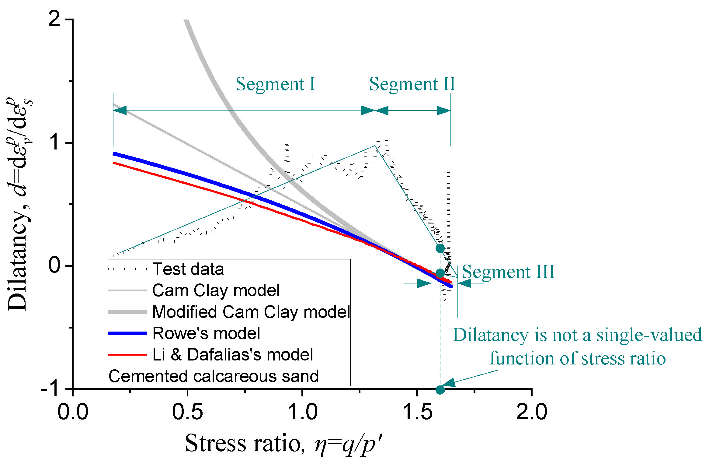
In Figure 14, we plot the stress-dilatancy curves predicted by four existing stress-dilatancy models. Obviously, the Modified Cam-Clay model has the largest deviation from the test data. While the other three stress-dilatancy models, the Cam-Clay model, Rowe’s model and Li&Dafalias’s model, are all approximately linear (see Figure 14), which cannot depict the three segments with different inclination angles of the stress-dilatancy curve. These things considered, the four predictions are quite different from the turning hook characteristics of the stress-dilatancy curve obtained from the test. While Figure 13 shows that our model can capture the turning hook feature of the true stress-dilatancy curve.

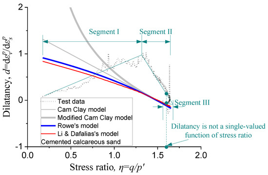
Figure 14. Comparison of predictions of stress−dilatancy relationship (${p^{\prime }}_0$ = 600 kPa).

The significance of considering the turning hook in the stress-dilatancy curve for crushable calcareous sand is that the more precise the turning hook simulation, the more precise the volumetric strain prediction.

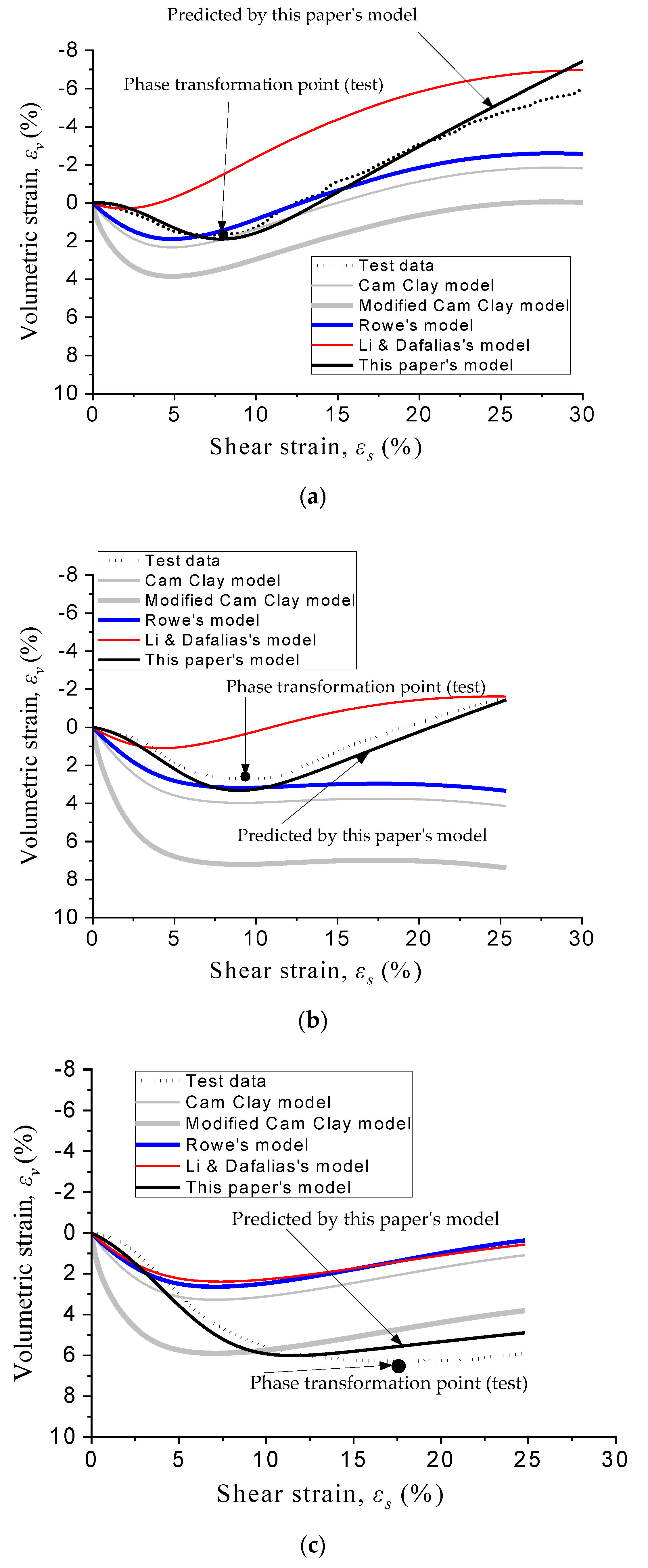
To show the significance of considering the turning hook, as shown in Figure 15, since our model depicts the turning hook of the stress-dilatancy curve, our model predicts the volumetric strain better than the other four existing stress-dilatancy models. Especially for the phase transformation point prediction, our model improves the case that the predicted transformation point appears much earlier than the test data, as shown by the other four existing stress-dilatancy models.

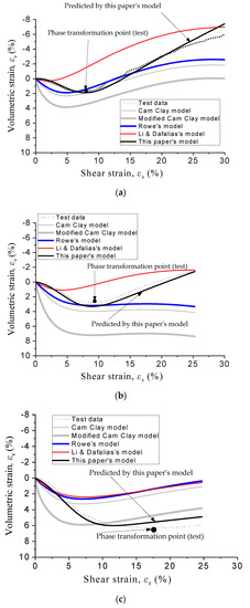
Figure 15. Comparison of predictions of volumetric strain: (a) ${p^{\prime }}_0$ = 100 kPa, (b) ${p^{\prime }}_0$ = 200 kPa, and (c) ${p^{\prime }}_0$ = 600 kPa.

5. Further Verification

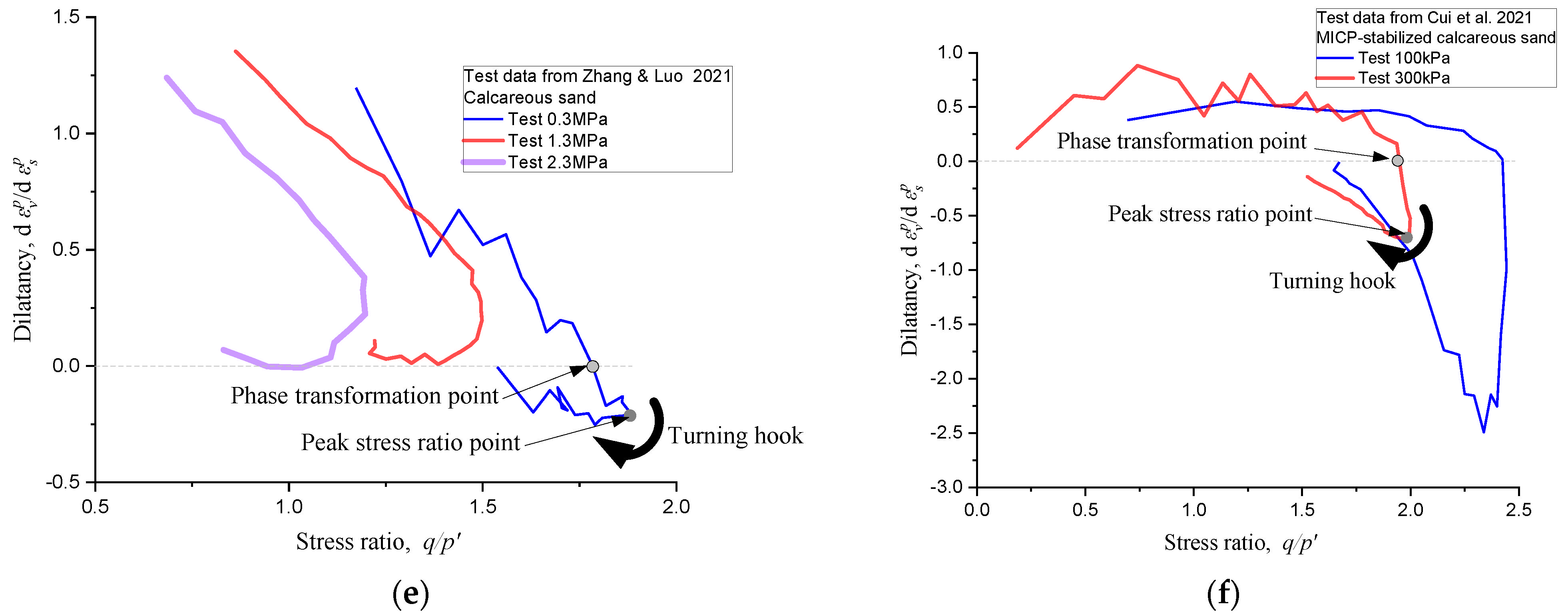
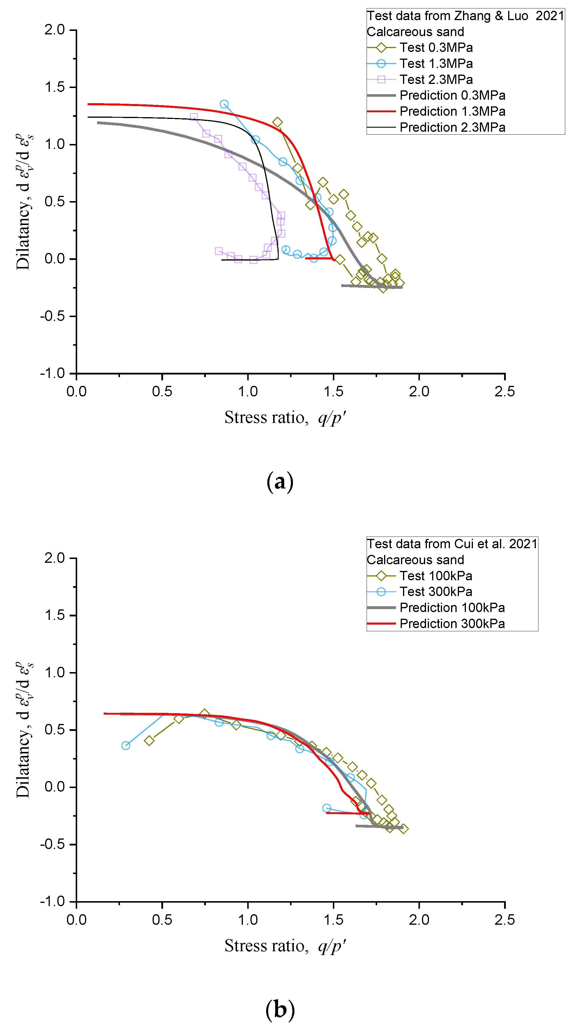
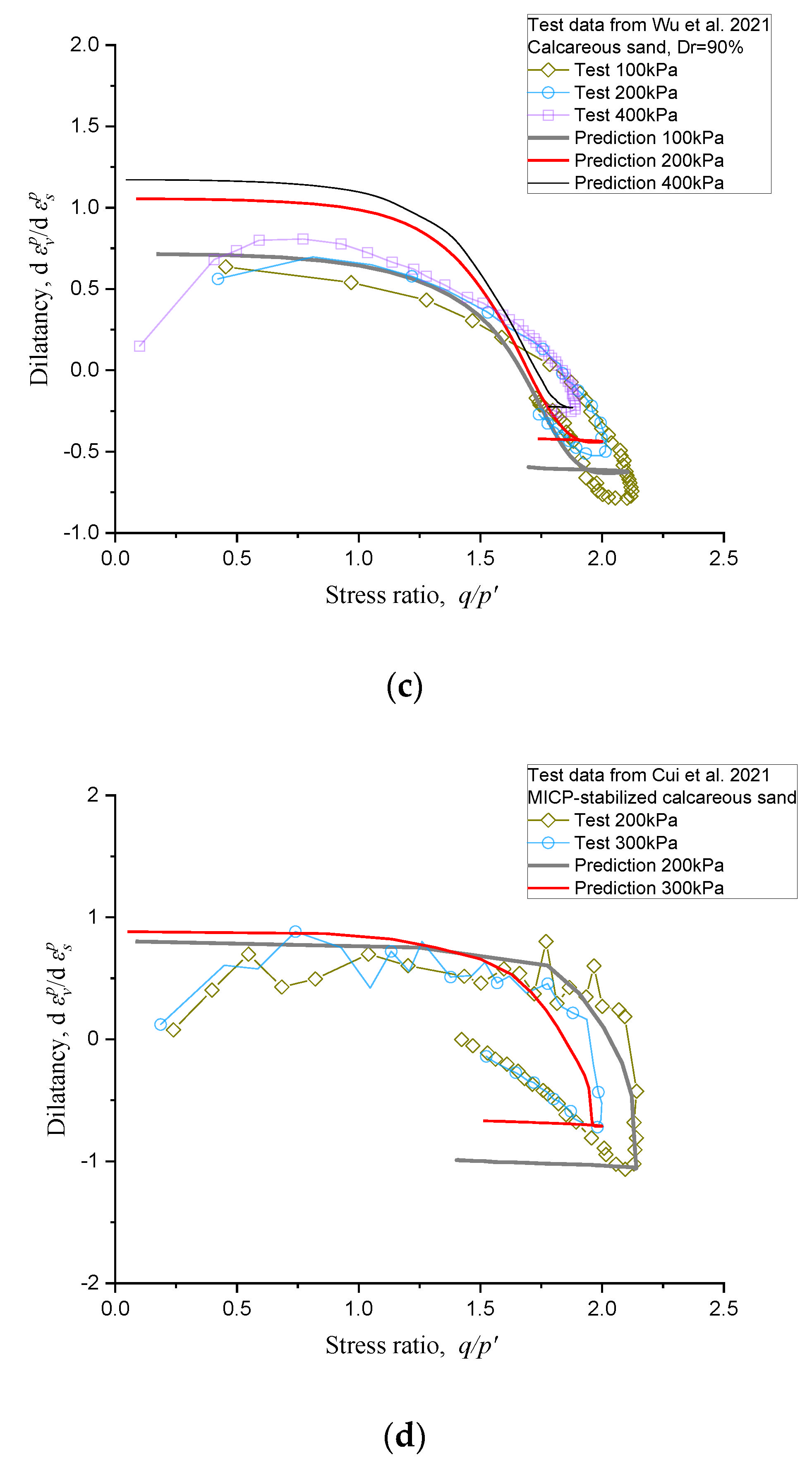
Previous literatures have shown that stress-dilatancy curves of crushable calcareous sands have turning hooks (see Figure 2, Wu et al., 2021 [1], Wang et al., 2022 [2], He et al., 2021 [3], Cui et al., 2021 [4] and Zhang & Luo 2021 [5]), and our developed model can be applied to the simulations of these calcareous sands (see the simulations in Figure 16).

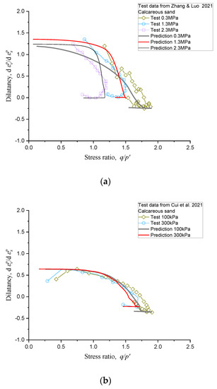
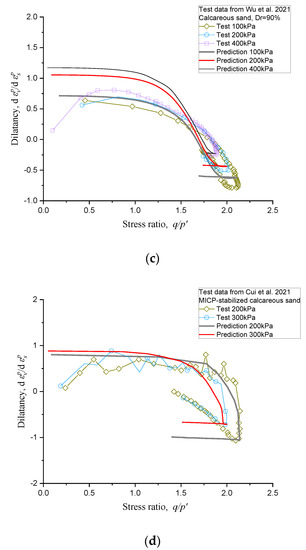
Figure 16. Predictions of the turning hooks of the stress−dilatancy curves: (a) calcareous sand (Zhang & Luo 2021 [5]), (b)calcareous sand (Cui et al., 2021 [4]), (c) calcareous sand (Wu et al., 2021 [1]), and (d) MICP-stabilized calcareous sand (Cui et al., 2021 [4]).

To further verify our stress-dilatancy model, Figure 16a–c showsour model’s predictions of stress-dilatancy relationships for three types of calcareous sands. MICP (microbially induced carbonate precipitation) is also an effective method to stabilize sand [32,33,34,35,36,37,38,39]. Previous literature [4] showed that MICP-stabilized calcareous sand exhibits the turning hook characteristics of the stress-dilatancy curve, and our model tries to simulate such turning hook (see Figure 16d). As shown in Figure 16, our model can capture the turning hooks of the true stress-dilatancy curves.

6. Conclusions

For calcareous sand, the previous stress-dilatancy models usually do not simulate the entire stress-dilatancy curve obtained from triaxial tests, i.e., they ignore the line segment after the peak stress ratio and miss the turning hook feature of the stress-dilatancy curve. While such ignored line segment corresponds to more than half of the whole loading process.

This paper presents a method to capture the turning hook feature of the stress-dilatancy curve, i.e., to simulate the stress-dilatancy curve more completely. Based on the first law of thermodynamics, we related dilatancy to breakage energy which was mapped from the stress-energy plane to the strain-energy plane. Then we established a relationship between stress ratio and shear strain. Based on the above two works, our stress-dilatancy model is conveniently established to capture the entire turning hook.

To verify our stress-dilatancy model, we performed triaxial tests on colloidal-silica-stabilized calcareous sand. Then we used the test data to show our model’s ability to capture the turning hook characteristics of the stress-dilatancy curve, while the other four existing stress-dilatancy models can not simulate such turning hook. Our model was also verified by MICP-stabilized calcareous sand and three types of calcareous sand in the literatures.

The implications of the findings for future research and potential applications are that: By mapping breakage-energy-related dilatancy from the stress-dilatancy plane to the strain-dilatancy plane, we can circumvent the non-single-valued problem of directly finding dilatancy as an analytical function of stress ratio. In addition, our method can easily capture the turning hook of calcareous sand’s stress-dilatancy curve, resulting in a more precise simulation of stress-dilatancy relationship. In addition, this more precise simulation of stress-dilatancy relationship allows for more precise prediction of volumetric strain.

References

- Wu, Y.; Li, N.; Wang, X.Z.; Cui, J.; Chen, Y.L.; Wu, Y.H.; Yamamoto, H. Experimental investigation on mechanical behavior and particle crushing of calcareous sand retrieved from South China Sea. Eng. Geol. 2021, 280, 105932. [Google Scholar] [CrossRef]
- Wang, X.; Shan, Y.; Cui, J.; Zhong, Y.; Shen, J.H.; Wang, X.Z.; Zhu, C.Q. Dilatancy of the foundation filling material of island-reefs in the South China Sea. Constr. Build. Mater. 2022, 323, 126524. [Google Scholar] [CrossRef]
- He, S.H.; Shan, H.F.; Xia, T.D.; Liu, Z.-J. The effect of temperature on the drained shear behavior of calcareous sand. Acta Geotech. 2021, 16, 613–633. [Google Scholar] [CrossRef]
- Cui, M.J.; Zheng, J.J.; Chu, J.; Wu, C.-C.; Lai, H.-J. Bio-mediated calcium carbonate precipitation and its effect on the shear behaviour of calcareous sand. Acta Geotech. 2021, 16, 1377–1389. [Google Scholar] [CrossRef]
- Zhang, J.; Luo, M. Dilatancy and critical state of calcareous sand incorporating particle breakage. Int. J. Geomech. 2020, 20, 04020030. [Google Scholar] [CrossRef]
- Schofield, A.; Wroth, C.P. Critical State Soil Mechanics; McGraw-Hill: London, UK, 1968; pp. 100–101. [Google Scholar]
- Roscoe, K.H.; Burland, J.B. On the Generalized Stress–Strain Behaviour of ‘Wet’ Clay. In Engineering Plasticity; Heyman, J., Leckie, F.A., Eds.; Cambridge University Press: Cambridge, UK, 1968; pp. 535–609. [Google Scholar]
- Rowe, P.W. The Stress–Dilatancy Relation for Static Equilibrium of an Assembly of Particles in Contact. Proc. R. Soc. Lond. Ser. A Math. Physicl Sci. 1962, 269, 500–527. [Google Scholar]
- Lu, Y.; Zhu, W.X.; Ye, G.L.; Zhang, F.M. A unified constitutive model for cemented/non-cemented soils under monotonic and cyclic loading. Acta Geotech. 2021; in press. [Google Scholar] [CrossRef]
- Gajo, A.; Cecinato, F.; Hueckel, T. Chemo-mechanical modeling of artificially and naturally bonded soils. Geomech. Energ. Envir. 2019, 18, 13–29. [Google Scholar] [CrossRef]
- Yan, W.M.; Li, X.S. A model for natural soil with bonds. Géotechnique 2011, 61, 95–106. [Google Scholar] [CrossRef]
- Yu, H.S.; Tan, S.M.; Schnaid, F. A critical state framework for modelling bonded geomaterials. Geomech. Geoeng. 2007, 2, 61–74. [Google Scholar] [CrossRef]
- Collins, I.F.; Hilder, T. A theoretical framework for constructing elastic/plastic constitutive models of triaxial tests. Int. J. Numer. Anal. Meth. Geomech. 2002, 26, 1313–1347. [Google Scholar] [CrossRef]
- Collins, I.F.; Muhunthan, B. On the relationship between stress–dilatancy, anisotropy, and plastic dissipation for granular materials. Géotechnique 2003, 53, 611–618. [Google Scholar] [CrossRef]
- Collins, I.F.; Muhunthan, B.; Qu, B. Thermomechanical state parameter models for sands. Géotechnique 2010, 60, 611–622. [Google Scholar] [CrossRef]
- Zhang, Z.; Li, L.; Xu, Z. A thermodynamics-based hyperelasticplastic coupled model unified for unbonded and bonded soils. Int. J. Plast. 2021, 137, 102902. [Google Scholar] [CrossRef]
- Xiao, Y.; Zhang, Z.C.; Stuedlein, A.W.; Evans, T.M. Liquefaction Modeling for Biocemented Calcareous Sand. J. Geotech. Geoenviron. Eng. 2021, 147, 04021149. [Google Scholar] [CrossRef]
- Wan, R.G.; Guo, P.J. A pressure and density dependent dilatancy model for granular materials. Soils Found. 1999, 39, 1–11. [Google Scholar] [CrossRef]
- Li, X.S.; Dafalias, Y.F. Dilatancy for cohesionlesssoils. Géotechnique 2000, 50, 449–460. [Google Scholar] [CrossRef]
- Hanley, K.J.; Huang, X.; O’Sullivan, C. Energy dissipation in soilsamplesduringdrained triaxial shearing. Géotechnique, 2018; 68, 421–433. [Google Scholar]
- Agapoulaki, G.I.; Papadimitriou, A.G. Rheological Properties of Colloidal Silica Grout for Passive Stabilization Against Liquefaction. J. Mater. Civ. Eng. 2018, 30, 04018251. [Google Scholar] [CrossRef]
- Gallagher, P.M.; Lin, Y. Colloidal silica transport through liquefiable porous media. J. Geotech. Geoenviron. Eng. 2009, 135, 1702–1712. [Google Scholar] [CrossRef]
- Fujita, Y.; Kobayashi, M. Transport of colloidal silica in unsaturated sand: Effect of charging properties of sand and silica particles. Chemosphere 2016, 154, 179–186. [Google Scholar] [CrossRef]
- Gallagher, P.M.; Conlee, C.T.; Rollins, K.M. Full-scale field testing of colloidal silica grouting for mitigation of liquefaction risk. J. Geotech. Geoenviron. Eng. 2007, 133, 186–196. [Google Scholar] [CrossRef] [Green Version]
- Gallagher, P.M.; Pamuk, A.; Abdoun, T. Stabilization of liquefiable soils using colloidal silica grout. J. Mater. Civ. Eng. 2007, 19, 33–40. [Google Scholar] [CrossRef]
- Conlee, C.T.; Gallagher, P.M.; Boulanger, R.W.; Kamai, R. Centrifuge Modeling for Liquefaction Mitigation Using Colloidal Silica Stabilizer. J. Geotech. Geoenviron. Eng. 2012, 138, 1334–1345. [Google Scholar] [CrossRef]
- Díaz-Rodríguez, J.A.; Antonio-Izarraras, V.M.; Bandini, P.; López-Molina, J.A. Cyclic strength of a natural liquefiable sand stabilized with colloidal silica grout. Can. Geotech. J. 2008, 45, 1345–1355. [Google Scholar] [CrossRef]
- Gallagher, P.M.; Mitchell, J.K. Influence of colloidal silica grout on liquefaction potential and cyclic undrained behavior of loose sand. Soil Dyn. Earthq. Eng. 2002, 22, 1017–1026. [Google Scholar] [CrossRef]
- Triantafyllos, P.K.; Georgiannou, V.N.; Pavlopoulou, E.; Dafalias, Y.F. Strength and dilatancy of sand before and after stabilisation with colloidal-silica gel. Géotechnique 2021, 72, 471–485. [Google Scholar] [CrossRef]
- Jin, W.F.; Tao, Y.; Wang, X.; Gao, Z. The effect of carbon nanotubes on the strength of sand seeped by colloidal silica in triaxial testing. Materials 2021, 14, 6119. [Google Scholar] [CrossRef]
- Jin, W.F.; Chen, R.Z.; Wang, X.; Cheng, Z.H. Effect of Wood Fiber on the Strength of Calcareous Sand Rapidly Seeped by Colloidal Silica. In Proceedings of the 1st International Conference on Advances in Civil Engineering and Materials and 1st World Symposium on Sustainable Bio-Composite Materials and Structrues, Nanjing, China, 9–11 November 2018. [Google Scholar]
- Konstantinou, c.; Biscontin, G.; Jiang, N.J.; Soga, K. Application of microbially induced carbonate precipitation to form bio-cemented artificial sandstone. J. Rock Mech. Geotech. 2021, 13, 579–592. [Google Scholar] [CrossRef]
- Cui, M.J.; Zheng, J.J.; Dahal, B.K.; Lai, H.J.; Huang, Z.F.; Wu, C.C. Effect of waste rubber particles on the shear behaviour of bio-cemented calcareous sand. Acta Geotech. 2021, 16, 1429–1439. [Google Scholar] [CrossRef]
- Zeng, H.; Yin, L.Y.; Tang, C.S.; Zhu, C.; Cheng, Q.; Li, H.; Lv, C. Tensile behavior of bio-cemented, fiber-reinforced calcareous sand from coastal zone. Eng. Geol. 2021, 294, 106390. [Google Scholar] [CrossRef]
- Xiao, Y.; Stuedlein, A.W.; Pan, Z.Y.; Liu, H.L.; Evans, T.M.; He, X.; Lin, H.; Chu, J.; Passen, L.A.V. Toe-bearing capacity of precast concrete piles through biogrouting improvement. J. Geotech. Geoenviron. Eng. 2020, 146, 06020026. [Google Scholar] [CrossRef]
- Liu, S.Y.; Dong, B.W.; Yu, J.; Cai, Y.Y.; Peng, X.Q.; Zhou, X.Q. Effect of different mineralization modes on strengthening calcareous sand under simulated seawater conditions. Sustainability 2021, 13, 8265. [Google Scholar] [CrossRef]
- Li, Y.J.; Guo, Z.; Wang, L.Z.; Ye, Z.; Shen, C.F.; Zhou, W.J. Interface shear behavior between MICP-treated calcareous sand and steel. J. Mater. Civ. Eng. 2021, 33, 04020455. [Google Scholar] [CrossRef]
- Li, Y.J.; Guo, Z.; Wang, L.Z.; Li, Y.L.; Liu, Z.Y. Shear resistance of MICP cementing material at the interface between calcareous sand and steel. Mater. Lett. 2020, 274, 128009. [Google Scholar] [CrossRef]
- Xiao, P.; Liu, H.L.; Xiao, Y.; Stuedleinc, A.W.; Evans, T.M. Liquefaction resistance of bio-cemented calcareous sand. Soil Dyn. Earthq. Eng. 2018, 107, 9–19. [Google Scholar] [CrossRef]
Publisher’s Note: MDPI stays neutral with regard to jurisdictional claims in published maps and institutional affiliations. |
© 2022 by the authors. Licensee MDPI, Basel, Switzerland. This article is an open access article distributed under the terms and conditions of the Creative Commons Attribution (CC BY) license (https://creativecommons.org/licenses/by/4.0/).