Numerical Simulation of Oil Spill in the Arctic Ice-Covered Waters: Focusing on Different Ice Concentrations and Wave’s Impacts

Abstract

The computational model was established to investigate the characteristics of oil spreading under arctic environments focusing on two aspects: ice concentrations and wave impacts. The ice field was constructed using the ice plates to compose three kinds of fixed arrays based on different ice concentrations of 90%, 60% and 0%. The wave was generated using the improved Jonswap spectrum method to control the focusing time, focusing location and focusing wave amplitude. The oil spreading’s movement was simulated and compared to the field experiment to verify the numerical model’s validity. The oil spill was trapped under the ice plates’ lower surface when the ice concentration was 60% or 90%, which had a spreading velocity slower than the non-ice water. The moving ice simulation was performed via the overset technique and coupled with the current, wind and wave. With ice drifting, the oil spreading was accelerated, leading to the presence of oil both on and under the ice surface. The ice was driven by the wave to affect the running details of the oil trajectory. These findings can be utilized for future oil spreading prediction when an oil spill accident occurs in the Arctic Ocean.

1. Introduction

Oil spill accidents are caused by ship collisions or human errors during loading-unloading and transportation operations, which have resulted in the pollution of the marine environment. Once the oil spill is injected into the open water, different types of oil transport occur, including drifting, spreading, dispersion, advection and sedimentation [1], causing severe damage to the marine organism and water environment if the protectors do not timely collect or treat the oil.

With the Arctic routine’s opening, ship traffic has become more and more frequent, and the oil spill accidents in the Arctic have also increased rapidly [2]. Due to the existence of the ice floes, the cold-water conditions are complicated. The oil spill simultaneously interacts with the atmosphere, seawater and ice, leading to the spreading behavior of the oil slick in this unique region is irregular [3,4]. The most significant characteristic of oil spreading in the ice-covered water is that the oil strives to find the channel between the ice plates. It spreads across through the edge of ice and fills as much of the gap as possible. That is to say, ice can trap the oil to reduce its spreading [5]. also It has also been reported that oil released under the ice cover would rise to the surface and remain without dispersing to any great extent in the water regions with broken ice covers [6]. Therefore, ice plays a crucial role in inhibiting the oil spreading and drifting, similar to a natural fence, and the diffusibility of oil depends on the ice concentrations.

Recently, some laboratory experiments were carried out to investigate the effect of the ice concentrations on oil spills. Different types of oil were utilized to observe the variation of oil thickness with different kinds of ice coverage [7]. The oil was continuously drifting between the ice packs in a slow and stable way. As the ice concentration increased, the inhibitory effect from ices was reinforced. Another experiment was carried out using a simplified ice pack model with various oil discharge rates and oil volumes [8]. The oil spill was found to gather under the ice and hold on. This is due to the interfacial tension between the oil and the ice plate, and the surface tension of the oil slick created a balance force, which acts in an arch manner against the buoyancy force. Although these field experiments were helpful to study the oil spill behavior, they were time-consuming, and the particular experimental conditions was subjected to site restrictions, funding constraints, scale effects and the generation technology of oil spills [9,10]. Flexible and efficiency approaches are urgently needed to study the oil spill in icy waters, and the numerical simulation is a good choice [11].

The oil spreading and drifting rate in icy waters was reported to be affected by four parameters, including the type of oil, ice concentration, the motion rate of ice and the amount of slush between the floes [12]. From a hydrodynamic perspective, the two most critical factors affecting the oil spreading are ice concentration and the motion rate of ice. The former is determined by the number of ice plates, while the latter is determined by the wave. It was discovered that the wave was attenuated after encountering the ice cover and the energy of wave fluctuation was transformed to ice, and the ice was driven by the wave to change the oil’s spreading trajectory [13,14]. Wave’s impacts are a necessary condition for assessing the severity of the oil spill in the Arctic Ocean. The wave transport may be impeded by the ice covers to cause the wave breaking; in turn, the ice suffers from the wave’s slamming to generate moving, causing the wake to have an irregular flow trend due to the ice-wave interaction. The stochasticity for waves exists objectively in nature and is difficult to analyze quantitatively. The advantage of using simulation to generate wave is that the focusing time and location can be controlled, and the wave’s impacts can be accurately analyzed on the ice body.

In numerical simulations, the linear and nonlinear methods are the main two approaches to generate waves. Based on the linear methods, ocean waves could be considered as the superposition of a large number of cosine waves with different periods and different random initial phases. The nonlinear methods could be realized via evolution equations such as the Kadomtsev-Petvashvili equation [15], the deep-water nonlinear Schrodinger equation [16] and the fully nonlinear equation [17]. However, the calculation for these nonlinear methods is too heavy to apply in realistic engineering. Thus, a linear super-location method for Jonswap wave spectrum was proposed to generate waves at fixed points in time [18].

In addition to the wave and ice, the wind, current and temperature must also be considered to establish a model close to the real arctic environment, which is helpful for accurately simulating the oil trajectory changes with time [19]. As the current oscillates back and forth, the oil is pushed onto the surface to contact with the ice. Both the mean oil trajectory and the oil spreading are sensitive to a threshold velocity for the withdrawal of oil from below ice floes [20]. The ultimate fate of the oil slick is determined by the oil-water-ice interfacial forces and the ice-water interface topography. In recent years, complex hydrodynamic factors, such as wind-wave interaction [21], surface tension [22] and ice motion [23], have been considered in oil spill experiments. Assuming that the crude oil cannot be entirely dissolved in water, the volume of fluid method (VOF) was adopted to track the oil flows of several immiscible fluids [24]. The Finite Volume Coastal Ocean Model was applied to predict the drift and diffusion processes for long-term oil spreading [25]. The oil movement direction was found to be determined by the current direction under the impact of surface waves and winds. The drift angle of different latitude conditions was also utilized to predict the oil slick trajectory by monitoring transport velocity and thickness of the oil slick [26]. The strong dependence of oil spill trajectory predictions on the presence of ice means that oil spill models that take ice into account are essential. Using the coupled ice-ocean model proposed by Tor [27], the simulation of oil fate and transport in ice-covered waters can be improved. Two oil-in-ice surface drift models were implemented to simulate the hypothetical oil spill in the Pechora Sea [28]. These methods could efficiently simulate the oil spill’s movement. However, their target environments only considered waters rather than moving ice. The spreading trajectory of oil slick in the presence of ice is completely different from that in non-ice-covered water, and its difficulty of predicting the oil trajectory will also be increased.

The objective of this work is to establish an oil spill model to predict the oil spreading and drifting trajectory among ice plates. The arctic geographical environments were simulated by considering two aspects: ice concentrations and wave impacts. The ice concentrations were limited as 90%, 60% and 0% by changing the ice plates’ arrangement. The waves were generated using the improved Jonswap spectrum method to control the focusing time, location and wave amplitude. The realizable K-Epsilon two-layer model was used to improve the accuracy, and the overset grids method was employed to simulate the ice motion. The effects of wind and current on the ice and hence on the oil spill were also studied by the phase interaction model and surface tension model. Three numerical validation experiments with different ice concentrations were carried out to verify this oil spill model’s effectiveness. The characteristics of oil spreading and drifting were also analyzed and compared in ice-covered waters and open waters. The result present a fundamental numerical experimental investigation of oil spreading and drifting in calm waters with floating ices and ice-covered waters with waves. The information can be collected and analyzed to predict the oil pollution area to provide an emergency measure for the Arctic Ocean’s oil spill treatment. In Appendix A, the symbols used in this paper are listed.

2. Theoretical Approach

2.1. Realizable K-Epsilon Two-Layer Model

For complex multiphase flow problems, the numerical prediction is generally performed by solving the Reynolds time-averaged N-S equation. The K-Epsilon turbulence model is a two-equation model that solves transport equations for the turbulent kinetic energy $k$ and the turbulent dissipation rate $\epsilon$ in order to determine the turbulent eddy viscosity. It has become the most widely used model for industrial applications. The K-Epsilon model was upgraded to the realizable K-Epsilon two-layer model in this work to simulate the oil spill in order to improve the accuracy.

The transport equations of kinetic energy $k$ and turbulent dissipation rate $\epsilon$ were expressed as Equations (1) and (2):

$$\frac{\partial }{\partial t}\left(\rho k\right)+\nabla ·\left(\rho k\overline{\nu }\right)=\nabla ·\left[\left(\mu +\frac{{\mu }_t}{{\sigma }_k}\right)·\nabla k\right]+P_k-\rho \left(\epsilon -{\epsilon }_0\right)+S_k$$

(1)

$$\frac{\partial }{\partial t}\left(\rho \epsilon \right)+\nabla ·\left(\rho \epsilon \overline{\nu }\right)=\nabla ·\left[\left(\mu +\frac{{\mu }_t}{{\sigma }_{\epsilon }}\right)·\nabla \epsilon \right]+\frac{1}{T_e}{C}_{\epsilon 1}{P}_{\epsilon }-C_{\epsilon 2}{f}_2\rho \left(\frac{\epsilon }{T_e}-\frac{{\epsilon }_0}{T_0}\right)+S_{\epsilon }$$

(2)

where $\rho$ is the density, $t$ is the time, $T_e$ is the large-eddy timescale, $T_0$ is the specific timescale, $\overline{\nu }$ is the mean velocity, $\mu$ is the dynamic viscosity, $S_k$ and $S_{\epsilon }$ are the user-specified source terms, ${\epsilon }_0$ is the ambient turbulence value in the source terms that counteracts turbulence decay and $f_2$ is the damping function given by:

$$f_2=\frac{k}{k+\sqrt{v\epsilon }}$$

(3)

${\sigma }_k$, ${\sigma }_{\epsilon }$, $C_{\epsilon 1}$ and $C_{\epsilon 2}$ are model coefficients. This study takes 1, 1.2 and 1.9 for ${\sigma }_k$, ${\sigma }_{\epsilon }$ and $C_{\epsilon 2}$, respectively. $C_{\epsilon 1}$ is specified by:

$$C_{\epsilon 1}=\max \left(0.43, \frac{\eta }{5+\eta }\right)$$

(4)

and

$$\eta =\frac{Sk}{\epsilon }$$

(5)

where $S$ is the average strain rate tensor. $P_k$ and $P_{\epsilon }$ are production terms, which can be obtained as:

$$P_k=f_c{G}_k+G_b+{\mathsf{{\rm Y}}}_M$$

(6)

$$P_{\epsilon }=f_{c}Sk+G_{\epsilon 3}{G}_b$$

(7)

where $C_{\epsilon 3}$ is the model coefficient, which can be taken as the constant of 1; $G_k$ is the turbulent production; $G_b$ is the buoyancy production; ${\mathsf{{\rm Y}}}_M$ is the compressibility modification; and $f_c$ is the curvature correction factor. ${\mu }_t$ is the turbulent eddy viscosity, which is calculated as:

$${\mu }_t=\rho C_{\mu }{f}_{\mu }kT$$

(8)

where $T$ is the turbulent time scale, $C_{\mu }$ is the critical coefficient and is taken as 0.09 for the two-layer model and $f_{\mu }$ is the enforced damping function to decrease the turbulent mixing near the walls.

The computation was divided into two layers in this model. In the layer next to the wall, the turbulent dissipation rate $\epsilon$ and the turbulent viscosity ${\mu }_t$ were specified as functions of wall distance. The values of $\epsilon$ specified in the near-wall layer were blended smoothly with the values computed from solving the transport equation far from the wall. The equation for the turbulent kinetic energy was solved across the entire flow domain. This explicit specification of $\epsilon$ and ${\mu }_t$ had a high accuracy of computing the region close to solid surfaces, for instance, analyzing the interactions between ice and water. The results were often as good or better.

2.2. Wave Generation Method

A prominent feature of the Arctic region is the presence of waves. Although the waves are not strong, they create a push on the ice that changes the trajectory of the oil spill. The improved Jonswap spectrum combined with the linear super-location method was used to simulate the weaker wave based on the wave dispersion theory. As for the wave transport on the sea surface, the linear wave equation can be expressed as:

$$\eta \left(x,t\right)={\displaystyle \sum }_{i=1}^M{a}_i\cos \left(k_{i}x-2\pi f_{i}t-{\phi }_i\right)$$

(9)

where $x$ and $t$ are the user-defined variances in function representing the wave location and time, respectively; $M$ is the number of component waves; $a_i$ is the amplitude of the component wave corresponding to the frequency $f_i$; $k_i$ is the wave number; and ${\phi }_i$ is the initial phase of the component wave.

In addition, $f_i$ and $k_i$ need to satisfy the linear dispersion relation equation as:

$${\omega }_i=2\pi f_i=\sqrt{k_{i}g\tan h{k}_{i}h}$$

(10)

where ${\omega }_i$ is the circular frequency, $g$ is the gravity acceleration (9.8 m/s²) and $h$ is the depth of water and can be obtained from the actual working conditions.

Assuming that the wave is focused at the assumed location of $x_b$ and the predetermined time $t_b$, the component waves are superimposed here and should satisfy the equations below:

$$\cos \left(k_i{x}_b-2\pi f_i{t}_b-{\phi }_i\right)=1$$

(11)

and

$${\phi }_i=k_i{x}_b-2\pi f_i{t}_b+2n\pi \left(n=0,\pm 1,\pm 2,\cdots \cdots \right)$$

(12)

Therefore, the wave surface equation can be expressed as:

$$\eta \left(x,t\right)={\displaystyle \sum }_{i=1}^M{a}_i\cos \left(k_i\left(x-x_b\right)-2\pi f_i\left(t-t_b\right)\right)$$

(13)

The improved Jonswap spectrum in this research can be described as:

$$a_i=AS\left(f_i\right)/{\displaystyle \sum }_{m=1}^{M_f}S\left(f_m\right)$$

(14)

where $a_i$ is the amplitude determined by the specific analog spectrum type of the wave, $A$ is the assumed focusing amplitude and $S\left(f\right)$ is the classic Jonswap spectrum proposed by Goda [29]:

$$S\left(f\right)={\beta }_J{H}_{1/3}^2{f}_p^4{f}^{-5}\exp \left[-\frac{4}{5}{\left(f/f_p\right)}^{-4}\right]·{\gamma }^{\exp \left[-{\left(\frac{f}{f_p}-1\right)}^2/2{\delta }^2\right]}$$

(15)

where $H_{1/3}$ is the significant wave height, $f_p$ is the center frequency corresponding to the uniform distribution interval $\left[f_i,f_n\right]$, $\delta$ is the spectral width coefficient obtained by the center circle frequency ${\omega }_p$, if $\omega \le {\omega }_p$, $\delta$ is taken as 0.07 if $\omega >{\omega }_p$, $\delta$ is taken as 0.09, $\gamma$ is the peak enhancement factor ranging from 1 to 7 with a mean value of 3.3 and ${\beta }_J$ is the function correlated with $\gamma$, as shown in Equation (16):

$${\beta }_J=\frac{0.06238}{0.23+0.0336\gamma -0.185{\left(1.9+\gamma \right)}^{-1}}·\left(1.094-0.01915\ln \gamma \right)$$

(16)

2.3. Overset Grids Method

Overset girds, also known as “Chimera” or overlapping grids, were used here to discretize a computational domain with several different meshes that arbitrary overlap each other. The key to overset grids’ calculations was to determine the data interpolation between sub-grids. The transfer relationship for overset grids included two steps: elimination and interpolation. The elimination was to shield some unnecessary or meaningless parts from the grid before the flow field calculation. The interpolation made the cells along the outer boundary of the overset body grid obtaining the variable values from the other component grid (donor grid), thus calculating the solution on each part of the grid. The interpolation formula is given as Equation (17):

$$\varnothing P_i={\displaystyle \sum }_{q=1}^{N_D}{\alpha }_{{\omega }_q}·\varnothing D_q$$

(17)

where $q$ is the cell unit; $P_i$ is the target point, $D_q$ is the donor point, $\varnothing P_i$ is the interpolated function value, $\varnothing D_q$ is the donor function value, ${\alpha }_{{\omega }_q}$ is the interpolation weight and $N_D$ is the number of total cells for all donors determined in domain.

The equation expressed the information transmission from the donor cells to the receptor cells corresponding to solving the mass and momentum equations from the overset girds to the background grids. A large number of grids were used in this work; thus, this overset method was suitable to enhance the solution’s accuracy.

3. Computational Model

In this paper, many environmental factors were considered in our oil spill model. On the one hand, it is difficult to build a complex and comprehensive model by integrating these factors; on the other hand, the calculation time is too long to perform the full-scale simulation due to the grid burden, accuracy requirements and computer performance limitations.

3.1. Concentrations of Ice Packs

The numerical experiment in this paper was established according to the parameters described in the tank model [8]. The saline water ices were cut into circular plates with a diameter of 10 cm and a thickness of 10 cm. The ice plates were herded into the test area and arranged with different ice concentrations. Three independent experiments were carried out with the oil discharge at a constant rate for case I (0% ice concentration), case II (60% ice concentration) and case III (90% ice concentration). The pool with no ice was adopted to simulate the static water in case I. In case II, the gap between the ice plates was 1 cm in the transverse direction and longitudinal direction. The ice plates were distributed as a square team in the center of water. In case III, the ice plates gathered and contacted each other. A small area of open water can be compassed by the edges of three circular plates. Thus, there was no accessible path on the water surface from one side of ice plate to the other side. No matter oil or water would not drift easily through the gap to converge together.

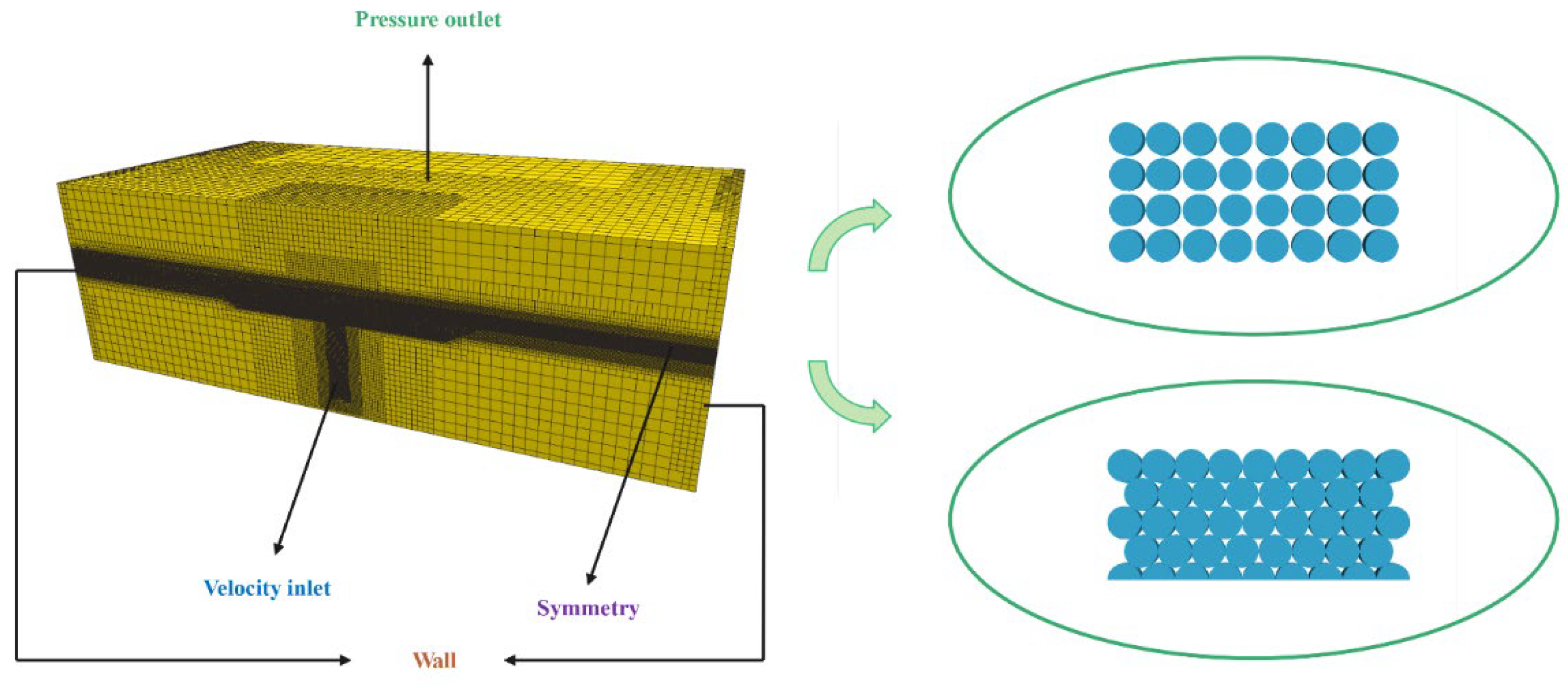
3.2. Grids and Boundary Conditions

It is difficult to replicate the realistic domain in a ratio of one to one. A small-scale flow field was constructed by reducing the magnitude of wave and ice plate based on the equivalent rules. The grids in the areas of free surface and oil jet were refined to capture the details of oil flow. The basic size of gird in the far field was 0.01 m. The grid size in refinement regions was densified by 12.5% and 6.25% in the X and Z directions based on the basic size. All domains were divided into a total of 2.25–3.45 million trimmed elements to ensure convergence during iteration. All the cases were computed using the K-Epsilon turbulence model introduced in Section 2.1. The phase interaction model was used to define the surface tension between water phase and oil phase. The air and water were divided by the VOF method. The ice plates were fixed to keep an upright floating status; thus, they were not dragged to change the position due to the coupling of wind and current. The boundary conditions of numerical model are shown in Figure 1. In order to reduce the computing time, only half of the domain was simulated because the ice was arranged symmetrically in the pool’s center plane and the oil jet was also in the middle of the bottom area. The bottom and edges of the pool were defined as the slip wall conditions. The oil jet was defined as a velocity inlet and submerged in water. The spreading of oil might be coupled with ice on the free surface. Hence, the height direction layers of the free surface were refined to 20 grids to capture the reaction details of oil and ice. The time step was limited to 0.001 s to ensure the computational convergence.

3.3. Moving Ice

A new grid generation strategy based on the overset technique was used to simulate the ice movement dynamically. The overset was utilized to create the information transmission from the background region to the overset region because it was suitable to simulate the small-amplitude movements of ice driven by weaker waves [30]. In total, 12 million grids were generated in the computational domain, including 4 million volume grids and 8 million overset grids. The overset region was used to embrace the ice to achieve the purpose of simulating the ice movement. The scale of overset grids was consistent with that of the background grids to guarantee the calculation convergence. The wave codes were applied in the oil spill model, while the refinement blocks were added near the free surface. The grids strategy of the free surface abided to the refinement principles as detailed descriptions: In the direction of the wave height, there at least were 20 layers of grids to be refined, and in the direction of the wavelength, there were at least 120 layers of grids to be refined. The case was performed with the total core processors of 50, 8 GB RAM, 64-bit operating computational system, 3.2 GHz. The wall clock time was about 2 weeks on an EPYC7552 computer.

4. Results and Discussion

Because the arctic wave is not strong, the ice’s drifting is slow. In realistic simulations, the encounter process between ice and oil can last for a long time, which is difficult to observe the ice-oil interactions. In order to capture the oil’s spreading details during the ice-oil coupling, the wave propagation in the realistic environment was divided into several short-range experiments to ensure the interactive phenomenon occurred.

The oil spill in a finite static water tank with different ice concentrations was simulated using the numerical model as mentioned above. The parameters are shown in

Table 1. Inputting parameters for different simulation cases.

Case No.	Case I	Case II	Case III
Ice concentration	0% (no ice)	60%	90%
Oil temperature (°C)	1	−0.5	−0.5
Oil viscosity (mPa·s)	95	190	145
Oil density	876	876	876
Discharge rate of oil (L/s)	0.00248	0.00193	0.00442
Saline temperature (°C)	0.2	−0.5	−0.5
Surface tension, oil/water (N/m)	0.0199	0.0205	0.0192
Surface tension, oil/air (N/m)	0.0229	0.0239	0.0225
Injecting time (s)	30	90	40

. Both ice plates and oil jet were arranged symmetrically in the water pool; thus, only half of far field was established numerically. The efficiency of parallel computers was found to improve significantly as the number of grids decreased.

4.1. Validation of Oil Slick Area in Case I

The changes of the oil slick area with a constant rate of oil discharge are illustrated in Figure 2. The oil slick area in case I was more extensive than those in case II and case III because the spreading oil was strongly restricted by the ice packs. The ice packs created a natural barrier to impede the oil movement. In open waters, after beginning to inject the oil, the oil was spilled from a fixed point and then extended to the wall of the pool similar to a circular disc. The initial oil slick area rapidly increased to 0.3 m² and then reached the equilibrium state due to the oil viscosity. The circular oil slick diameter was measured to be about 1.05 m at the time of 30 s, and the oil slick area was smaller than 0.5 m². These data corresponded well to the results of the water pool experiment (see Figure 3). Because the current and wind were not considered in case I, the simulation of oil spreading was regarded as performed in static water. The oil was found to move along the horizontal and vertical directions, which was consistent with the results of the static water experiment obtained by Fingas [5]. The distribution of oil in the vertical plane was shown in Figure 4. The droplets were driven by the buoyancy to up-float for a certain distance in a symmetric distribution way, leading to an oscillation of the free surface. The oil slick was promoted by the oscillation to further spread. The thickness of oil slick reached about 0.015–0.02 cm at last, which was also similar to the result of the Otsuka’s field tests corresponding to the thickness of oil slick was 0.01 cm when the ice concentration was 0%.

4.2. Validation of Oil Slick Area in Case II

The oil trended to spread along the water path that was not occupied by ice because the spreading velocity of the surface oil slick was faster than beneath the ice. In case II, the ice plates were set on the free surface using an 8 × 4 arrangement scheme and the distance between two plates was less than 1 cm, meaning that most of water surfaces were covered by ice. Therefore, only a small part of oil was squeezed to drift through the narrow gaps among the ice plates as shown in Figure 5. Most of the oil was covered by ice plates and moved tardily along the ice’s lower surface, which again illustrates that the oil spreading was limited by ice plates. The final area of oil slick reached 0.07 m² at the time of 90 s, which was smaller than that in case I. The variation of oil area indicated that oil spill in icy waters was significantly different from that in open waters, and this result was consistent with the inference obtained by Afenyo [1].

The CFD outputs were compared with the water pool experiment results as shown in Figure 6. Before the time of 50 s, the oil slick area in CFD results were close to that in the Experimental Fluid Dynamics (EFD) results, while after the time of 50 s, there was a medium deviation between CFD and EFD results. This deviation increased continuously with time. It was analyzed that the ice plates were assumed as an ideal model without melting in CFD simulation. However, in the actual pool experiment, the ice plates must be melted inevitably. The ice slush produced by melted ice could accelerate the oil to spread in the water pool. Because the effect of ice slush was ignored, the oil slick area in CFD was reduced when compared with the theory. The oil movement in the vertical plane is shown in Figure 7. Most of the oil spill remained beneath the ice plates, and the distance of the oil slick’s horizontal spread was less than 0.55 m at the time of 30 s. The final oil slick thickness was 0.2 cm in case II, while it was 0.22 cm in the Otsuka’s test with 60% ice concentration. This showed a perfect consistency between our simulation results and the water pool experiment results. Although the injecting oil volume in case II was higher than in case I, the oil spreading distance in case II was less than that in case I because of the existence of ice blocking. Moreover, ice can affect the water flow and change the oil’s movement to spread around the edges of ice plates, which was also observed by Faksness [31].

4.3. Validation of Oil Slick Area in Case III

The arrangement of ice plates was changed to increase the ice concentration to 90% in case III. The ice plates were fixed to contact with each other, which made the area for open water smaller. Some triangle water regions could be generated, as shown in Figure 8. Because the water regions were enclosed, the oil spill could not spread through the gaps among the ice plates to reach these regions; therefore, the oil slick had to spread beneath the lower surface of ice plates to reach each of the triangle regions. Finally, the oil was trapped in these triangle regions among the ice plates, and the oil slick area was only 0.004–0.014 m². This confirmed that the increased ice coverage caused the oil spreading to be restricted. The dimensions of the oil area in case III clearly decreased compared to those in cases I and II. The final oil slick areas with ice concentrations of 60% and 90% had a 6-times and 300-times lower ice concentration than that in open water, respectively, indicating that the greater the ice concentration was, the fewer the final oil slick area was. Comparison of oil slick area between CFD and EFD is shown in Figure 9, and the CFD results agreed with the EFD results, which indicate that the numerical model in this work is effective to simulate oil spill in icy waters. The distribution characteristics of oil with time in the vertical plane are shown in Figure 10. The oil droplets were driven by buoyancy to up-float the lower surface of ice plates (0–0.2 m under the water surface) and trapped there, so that only a very small part of oil could be seen on the water surface. The thickness of oil slick decreased from 8 cm to 0.9 cm. In Otsuka’s water pool experiment with 90% ice concentration, the final oil slick thickness was about 0.88 cm, similar to our results, which indicates that the accuracy of the numerical spreading model is excellent in this work.

4.4. Accuracy Analysis of Wave

For experimental observations, it is difficult to execute large deployments on the field due to the cost of devices [32]. In order to obtain enough available data from measurements, we used a refined wave tank model to replace the open wave field. Considering the nonlinearity of waves in the Arctic region induced by wind and current, the expected waves were generated using the wave superposition method to derive the synthetic waves. The external environmental loads provided by synthetic waves are controllable, and the amount of calculation can be reduced efficiently.

The wave generation model was tested for validating accuracy under different conditions, such as focusing time, focusing location and focusing wave amplitude, using the user-defined codes. Three groups of verification with different assumed amplitudes were conducted in simulations. The wave amplitude was assumed as 0.03 m, 0.05 m and 0.08 m, respectively. The maximum wave steepness was limited at 0.22, conforming to the standard of unbroken wave steepness. The main particulars of the wave are shown in

Table 2. Parameters associated with the waves.

Case No.	A	B	C
Focusing amplitude (m)	0.03	0.05	0.08
Wave steepness	0.083	0.14	0.22
Number of composition waves	30	30	30
Frequency Range (Hz)	0.6–1.06	0.6–1.06	0.6–1.06
Center frequency (Hz)	0.83	0.83	0.83
Focusing time (s)	2	2	2
Focusing location (m)	2.5	2.5	2.5
Error (%)	1.16	2.96	4.88

.

In this study, the requirement for wave validation was to ensure the maximum wave could appear at the preset focusing location under the premise that the assumed wave amplitude had been obtained. The surface elevations and maximum wave amplitudes were much closer to those reported by theoretical results because their errors were within 5%, and the largest wave appeared at the predestined focusing time (t = 2 s), as shown in Figure 11. The wave weakened with time, and it tended to be stable after 6 s because the wave energy was transformed to the current. The surface elevations were symmetrical before and after the appearing location of the maximum wave. These features were all in line with expectations and validated in actual measured data by Mori [33]. In this work, the assumed focusing time in three cases were all 2 s, while the actual focusing time was 2.05 s, 2.07 s and 2.07 s corresponding to case A, B and C, respectively. The results showed that all the actual focusing times were controlled close to the expected point, and the improved wave generation method as mentioned in Section 2.2 could be effectively utilized to simulate the wave in the Arctic waters.

4.5. Prediction of Oil Spreading in Icy Waters

The behavior of an oil spill depends on the environmental conditions. Once the oil is leaked into water from the ship, it is affected by the wave fluctuation and wind-current coupling. The wave is an essential factor because it might drive the ice to carry out a free motion; hence, the oil trajectory would be changed to follow the ice drift. Accordingly, the wave’s impacts were considered in this numerical model to realistically analyze the reactions among the oil, ice, wave, current and wind in the arctic. An ice disc with 1.5 m diameter and 0.2 m thickness was adopted, and a 3-D far-field of 6 m × 3.5 m was established as the computational region. Crude oil was injected into the region from the inlet side at the rate of 3 m/s. The ice was pushed by waves and current to drift together with the oil, as shown in Figure 12. The results of oil spill movement indicated that oil and ice tended to move in the same direction but at different speeds due to the existence of waves.

At the initial stage, the wave was stable as shown in Figure 12a. After 2 s, the maximum wave appeared, leading to a water bulge on the free surface, and this bulge impacted on the front part of the ice pack, as shown in Figure 12b. Under the action of the wave, the ice pack moved along the same direction with the wave; until the time of 4 s, the maximum wave moved ultimately through the ice and tended to be stable. At this time, the horizontal moving distance of the ice mass center was 5.1 m. According to the energy conservation, the energy required by the ice movement came from the wave. The wave encountered the ice and delivered energy to the ice, causing the ice’s front end to sink under the water; then, the wave weakened and had insufficient energy to cause the ice to sink when it moved to the ice pack’s back end. Therefore, the slamming loads on the front end and back end of the ice were different, causing the ice to heave along Y-axis and pitch along Z-axis. The ice apparently heaved and pitched, corresponding to the trim angle of 8° and the ice mass center vertical offset of 0.75 m, respectively, as shown in Figure 12c,d.

Some oil spread onto the ice surface and moved forward with the wave; some oil was trapped beneath the ice and entrained in the current vortex caused by the ice’s heaving and pitching. The vortex scale was basically constant, and the entrained oil amount was 0.007 m³. The amount of oil on the water’s upper layer was 0.065 m³, accounting for 90.2% of the total amount of oil spill. This result was similar to Guo’s findings [21], which reported that about 90% of the oil was found on the water up-layer (0–0.2 m of the free surface). Although the oil spread simultaneously on and beneath the ice, the spreading rates of these two parts were different. During the oil spreading period, the rate of oil drifting on the water surface was faster than that moving under the ice. In this work, the oil drifting rate on the water surface was about 1.4 m/s, and the oil drifting rate under the ice’s lower surface was only about 0.08 m/s. At the time of 4 s, the drifting distance and maximum thickness of the oil slick were 5.86 m and 0.18 m, respectively. The maximum thickness appeared in the water region without ice. The wind acted on the water surface and accelerated the wave’s movement. The maximum peak amplitude of wave was 0.32 m, and the time that the maximum wave acted on ice body was 2.2 s. The vortex remained close to the ice’s front end, and its size no longer increased with time.

The oil slick area on the ice’s upper surface was extracted from the model and is shown in Figure 13. The oil slick area increased with time, and the oil spreading caused the water surface of 2 m² to be polluted at the time of 4–5 s after the oil leakage. The inflection point appeared at 3 s, indicating that a part of oil drilled under the pack ice and became trapped under the ice’s lower surface. The ice moved upward and downward by the wave’s impacts to exacerbate the collision of the ice edge and oil. In such a way, the oil slick had the tendency to break into some small droplets and floated on the water surface, which increased the difficulty of emergency treatment.

5. Conclusions

The numerical model based on arctic environmental factors was developed to study the drifting and spreading characteristics of the oil spill in icy waters. First, the numerical oil spill models, including three cases corresponding to ice concentrations of 0%, 60% and 90%, were verified through comparison with the water pool experimental test. The results showed that the oil tended to spread beneath the ice lower-surface and then become trapped in the open water area circumscribed by the ice plates. As the ice concentration increased, the capacity of oil spreading decreased. Moreover, the quantitative comparison of the oil slick area between CFD and EFD indicated that this integrative numerical model could reasonably predict the oil spill area in icy waters. Second, the wave was generated in the simulation using the improved Jonswap spectrum method and was verified to ensure that the maximum wave appeared at the preset focusing location. Finally, the wind, current, wave and moving ice were comprehensively considered and simulated in one oil spill model. The ice movement was implemented by the overset technique. The pitch and heave motions were monitored to capture the details of the oil spreading trajectory. The results showed that the ice was driven by the wave to affect the running direction of the oil trajectory. The oil beneath the water was entrained to form an oil vortex near the front-end of pack ice, and the ice moved upward and downward by the wave’s impacts to exacerbate the collision of ice edge and oil. Most of the oil broke into small droplets and floated on the water surface. The information can be collected and analyzed to predict the oil pollution area to provide an emergency measure for the Arctic Ocean’s oil spill treatment.

Our future work will be focused on precisely predicting the trajectory of oil spill under the coupled ice-ocean condition and quantitatively measuring the oil slick to provide an emergency measure in real operations.

References

1. Afenyo, M.; Veitch, B.; Khan, F. A state-of-the-art review of fate and transport of oil spills in open and ice-covered water. Ocean Eng. 2016, 119, 233–248. [Google Scholar] [CrossRef]
2. Wang, K.G.; Leppäranta, M.; Gästgifvars, M.; Vainio, J.; Wang, C.X. The drift and spreading of the Runner 4 oil spill and the ice conditions in the Gulf of Finland, winter 2006. Est. J. Earth. Sci. 2008, 57, 181–191. [Google Scholar] [CrossRef]
3. Løset, S.; Shkhinek, K.; Gudmestad, O.T.; Strass, P.; Michalenko, E.; Frederking, R.; Kärnä, T. Comparison of the physical environment of some Arctic seas. Cold Reg. Sci. Technol. 1999, 29, 201–214. [Google Scholar] [CrossRef]
4. Valdez Banda, O.A.; Goerlandt, F.; Kuzmin, V.; Kujala, P.; Montewka, J. Risk management model of winter navigation operations. Mar. Pollut. Bull. 2016, 108, 242–262. [Google Scholar] [CrossRef]
5. Fingas, M.; Hollebone, B.P. Oil Behavior in Ice-Infested Waters. In Proceedings of the 36th AMOP Technical Seminar on Environmental Contamination and Response, Ottawa, ON, Canada, 4–6 June 2013. [Google Scholar] [CrossRef]
6. Glaeser, J.L.; Vance, G. A study of the behaviour of oil spills in the arctic. In Proceedings of the Offshore Technology Conference, Houston, TX, USA, 30 April–2 May 1972. [Google Scholar] [CrossRef] [Green Version]
7. Liu, B.X.; Zhang, W.; Han, J.S.; Li, Y. Tracing illegal oil discharges from vessels using SAR and AIS in Bohai Sea of China. Ocean Coast. Manag. 2021, 211, 105783.1–105783.9. [Google Scholar] [CrossRef]
8. Otsuka, N.; Ogiwara, K.; Kanaami, K.; Takahashi, S.; Saeki, H. Experimental study on spreading of oil spilled among pack ice. Proc. Civ. Eng. Ocean. 2011, 18, 767–772. [Google Scholar] [CrossRef] [Green Version]
9. Liu, S.X.; Hong, K.Y. Physical investigation of directional wave focusing and breaking waves in wave basin. China Ocean. Eng. 2005, 19, 21–35. [Google Scholar]
10. Kachulin, D.; Dyachenko, A.; Zakharov, V. Probability Distribution Functions of freak-waves: Nonlinear vs linear model. Stud. Appl. Math. 2016, 137, 189–198. [Google Scholar]
11. Ning, D.Z.; Zang, J.; Liu, S.X.; Eatock Taylor, R.; Teng, B.; Taylor, P.H. Free-surface evolution and wave kinematics for nonlinear uni-directional focused wave groups. Ocean. Eng. 2009, 36, 1226–1243. [Google Scholar] [CrossRef]
12. Gjøsteen, J.K.; Løset, S. Laboratory experiments on oil spreading in broken ice. Cold Reg. Sci. Technol. 2004, 38, 103–116. [Google Scholar] [CrossRef]
13. Yapa, P.D.; Li, Z. Simulation of oil spills from underwater accidents I: Model development. J. Hydraul. Res. 1997, 35, 673–688. [Google Scholar] [CrossRef]
14. Faksness, L.G.; Brandvik, P.J.; Daae, R.L.; Leirvik, F.; Børseth, J.F. Large-scale oil-in-ice experiment in the Barents Sea: Monitoring of oil in water and MetOcean interactions. Mar. Pollut. Bull. 2011, 62, 976–984. [Google Scholar] [CrossRef]
15. Pelinovsky, E.; Talipova, T.; Kharif, C. Nonlinear-dispersive mechanism of the freak wave formation in shallow water. Phys. D Nonlinear Phenom. 2000, 147, 83–94. [Google Scholar] [CrossRef]
16. Andonowati; Karjanto, N.; van Groesen, E. Extreme wave phenomena in down-stream running modulated waves. Appl. Math. Model. 2007, 31, 1425–1443. [Google Scholar] [CrossRef]
17. Li, B.; Fleming, C.A. A three dimensional multigrid model for fully nonlinear water waves. Coast. Eng. 1997, 30, 235–258. [Google Scholar] [CrossRef]
18. Dommermuth, D.G.; Lewis, C.D.; Tran, V.H.; Valenciano, M.A. Direct simulations of wind-driven breaking ocean waves with data assimilation. In Proceedings of the 30th Symposium on Naval Hydrodynamics, Hobart, Tasmania, Australia, 2–7 November 2014. [Google Scholar] [CrossRef]
19. Deslauriers, P.C.; Martin, S.C. Behavior of The Bouchard #65 Oil Spill in The Ice-Covered Waters of Buzzards Bay. 1. In Proceedings of the Offshore Technology Conference, Houston, TX, USA, 7–10 May 1978. [Google Scholar] [CrossRef]
20. Lars, A.; Höglund, A.; Axell, L.; Lensu, M.; Liungman, O.; Mattsson, J. Oil drift modeling in pack ice–sensitivity to oil-in-ice parameters. Ocean. Eng. 2017, 144, 340–350. [Google Scholar]
21. Guo, W.J.; Wang, Y.X. A numerical oil spill model based on a hybrid method. Mar. Pollut. Bull. 2009, 58, 726–734. [Google Scholar] [CrossRef]
22. Li, W.; Liang, X.; Lin, J.G. Mathematical Model and Computer Simulation for Oil Spill in Ice Waters Around Island Based on FLUENT. J. Comput. 2013, 8, 1027–1034. [Google Scholar] [CrossRef]
23. Li, W.; Liang, X.; Lin, J.G.; Guo, P.; Ma, Q.; Dong, Z.P.; Liu, J.M.; Song, Z.H.; Wang, H.Q. Numerical Simulation of Ship Oil Spill in Arctic Icy Waters. Appl. Sci. 2020, 10, 1394. [Google Scholar] [CrossRef]
24. Phuc, P.V.; Yoshida, A.; Imazu, Y.; Hasebe, M. Three dimensional multiphase flow analysis of tsunami with oil spill using VOF method. Coast. Eng. 2016, 72, 415–420. [Google Scholar] [CrossRef] [Green Version]
25. Li, H.; Li, Y.; Li, C.; Wang, G.S.; Xu, S.S.; Song, J.; Zhang, S. Numerical simulation study on drift and diffusion of Dalian Oil Spill. In Proceedings of the IOP Conference Series Earth and Environmental Science, Sanya, China, 21–23 November 2016. [Google Scholar] [CrossRef]
26. Zanier, G.; Petronio, A.; Armenio, V. The effect of Coriolis force on oil slick transport and spreading at sea. J. Hydraul. Res. 2017, 55, 409–422. [Google Scholar] [CrossRef]
27. Tor, N.; Beegle-Krause, C.J.; Skancke, J.; Nepstad, R.; Reed, M. Improving oil spill trajectory modelling in the Arctic. Mar. Pollut. Bull. 2019, 140, 65–74. [Google Scholar]
28. Aguiar, V.D.; Dagestad, K.F.; Hole, L.R.; Barthel, K. Quantitative assessment of two oil-in-ice surface drift algorithms. Mar. Pollut. Bull. 2022, 175, 113393. [Google Scholar] [CrossRef] [PubMed]
29. Goda, Y. A comparative review on the functional forms of directional wave spectrum. Coast. Eng. J. 1999, 41, 1–20. [Google Scholar] [CrossRef]
30. Carrica, P.M.; Fu, H.; Stern, F. Computations of self-propulsion free to sink and trim and of motions in head waves of the KRISO Container Ship (KCS) model. Appl. Ocean Res. 2011, 33, 309–320. [Google Scholar] [CrossRef]
31. Faksness, L.G.; Brandvik, P.J. Distribution of water soluble components from oil encapsulated in Arctic sea ice: Summary of three field seasons. Cold Reg. Sci. Technol. 2008, 54, 106–114. [Google Scholar] [CrossRef]
32. Rabault, J.; Sutherland, G.; Ward, B.; Christensen, K.H.; Halsne, T.; Jensen, A. Measurements of waves in landfast ice using inertial motion units. IEEE Trans. Geosci. Remote Sens. 2016, 54, 6399–6408. [Google Scholar] [CrossRef]
33. Mori, N.; Liu, P.C.; Yasuda, T. Analysis of freak wave measurements in the Sea of Japan. Ocean Eng. 2002, 29, 1399–1414. [Google Scholar] [CrossRef]
Figure 1. Details of the domain grids and arrangements of ice plates.
Jmse 11 00114 g001
Figure 2. The variation of oil area with time for case I (no ice). (a) Time = 10 s; (b) time = 20 s; (c) time = 30 s.
Jmse 11 00114 g002
Figure 3. Comparison of the oil slick areas of CFD and EFD in case I.
Jmse 11 00114 g003
Figure 4. Oil trajectory in the vertical plane of case I. (a) Time = 10 s; (b) time = 20 s; (c) time = 30 s.
Jmse 11 00114 g004
Figure 5. The variation of oil area with time for case II (60% ice concentration). (a) Time = 10 s; (b) time = 20 s; (c) time = 30 s.
Jmse 11 00114 g005
Figure 6. Comparison of the oil slick areas of CFD and EFD in case II.
Jmse 11 00114 g006
Figure 7. Oil trajectory in the vertical plane of case II. (a) Time = 10 s; (b) Time = 20 s; (c) Time = 30 s.
Jmse 11 00114 g007
Figure 8. The variation of oil area with time for case III (90% ice concentration). (a) Time = 10 s; (b) time = 20 s; (c) time = 30 s.
Jmse 11 00114 g008
Figure 9. Comparison of the oil slick areas of CFD and EFD in case III.
Jmse 11 00114 g009
Figure 10. Oil trajectory in the vertical plane of case III. (a) Time = 10 s; (b) time = 20 s; (c) time = 30 s.
Jmse 11 00114 g010
Figure 11. Time histories of surface elevation. (a) Case A; (b) case B; (c) case C.
Jmse 11 00114 g011
Figure 12. Oil spreading with the coupling of the wave and ice motion in icy waters. (a) Time = 1 s; (b) time = 2 s; (c) time = 3 s; (d) time = 4 s.
Jmse 11 00114 g012
Figure 13. Prediction of the oil slick area in icy waters.
Jmse 11 00114 g013