Abstract
The aim of this study is to better understand cross-reef wave-driven current characteristics, which are crucial to biological, ecological, and geomorphological processes within coral reefs. This study reports a set of new wave flume measurements to assess flow along the water depth and across a fringing reef profile under the action of a plunging breaker. Laboratory results are presented in view of cross-reef variations in both the wave height and the mean water level (MWL); the vertical profiles of wave-averaged mean currents below the wave trough and along the reef are also presented. To resolve the two-dimensional vertical (2DV) flow characteristics across the reef, Reynolds-Averaged Navier–Stokes (RANS) equations were solved using k-ω SST closure, modified to improve stability, and a Volume of Fluid (VOF) approach was used to capture the water surface. This numerical model was first validated via experimental measurements in view of waves and flows. It was then used to analyze the cross-reef distributions of the mean flow field, turbulent kinetic energy (TKE), and Reynolds shear stress across the reef.
1. Introduction
Fringing reefs are pervasive in tropical or subtropical oceans among various reef types. A typical fringing reef profile consists of a steeper fore-reef slope as well as a relatively horizontal reef flat that is attached directly to the coast. Over the past few decades, waves have been widely regarded as the dominant ocean force that controls hydrodynamics across reefs [1]. When incident waves interact with fringing reefs, they deform due to wave shoaling when propagating over the fore-reef. After this, they break near the reef’s edge, causing a drastic dissipation of wave energy and resulting in a rise in the mean water level, i.e., a wave-induced setup. The wave setup is driven from the cross-shore current on the reef flat. For an idealized fringing reef with no lateral reef flat rip channels, the shoreward wave-driven current can only be balanced by an undertow [2,3]. A better interpretation of the flow characteristics across the reef is vital to further understanding ecological (it transports nutrients, thus determining coral growth), biological (it conveys coral larval, thus maintaining coral breeding), and geomorphological (it moves sediments, thus affecting coral health) processes [4]; hence, it is beneficial to reef conservation projects.
Compared with an abundance of field investigations into wave and current characteristics in reef environments [5,6,7,8], laboratory investigations of wave-driven flow characteristics across reefs are limited in the literature. Importantly, Gourlay [9] conducted a pioneering investigation that measured waves and flows based on a horizontally one-dimensional (1DH) laboratory reef profile. It was found that a wave-generated flow across the reef was relatively weaker as reef submergence was either small or large. The maximum flow was observed with an intermediate water depth. Until recently, Yao et al. [10] performed wave flow measurements along a quasi-horizontally two-dimensional (referred to as quasi-2DH) reef–channel system in a wave flume. The current through the rip channel was modeled by linking the lagoon to the offshore side via a pipe. However, the alongshore hydrodynamics of the reef flat and the lagoon were not considered. They found that a wave-forced shoreward flow on the reef flat was balanced by an offshore-directed current in the channel. Subsequently, Zheng et al. [11] reported a series of wave basin experiments to investigate wave-induced circulation in a full 2DH reef–lagoon–channel system. A clear circulation cell (a continuous onshore current that travels along the reef flat before entering the lagoon and then returns back to the open sea via the rip channel) was identified, which is in agreement with some field investigations [6,7]. Nevertheless, wave-driven currents in all the above studies were usually obtained from the middle depths of limited sampling locations. To remedy such deficiencies in the flow measurement over reef profiles, Yao et al. [3] conducted a pioneering study to measure the flow variation along the water depth and around the reef surf zone based on a fringing reef profile. They found a 2DV circulation consisting of a wave-driven forward current and an underneath return flow (undertow) in the surf zone near the reef edge. Subsequently, Yao et al. [4] measured the vertical distribution of a wave-driven flow for a barrier reef configuration by considering the presence of a tidal current. They reported that the cross-reef mean current in the surf zone was primarily onshore-directed for the barrier reef case; a larger seaward/shoreward current below the wave trough could be observed as waves traveled on the ebb/flooding tidal current. However, wave-driven flow characteristics along the water depth and over the entire reef flat were not investigated in the above experiments.
In the literature, numerical models are powerful tools to reveal wave and current characteristics in different reef environments. For laboratory-scale reef hydrodynamic modeling, two groups of phase-resolving models are the most popular. The first group is based on the Boussinesq equations. Boussinesq-type models can maintain both wave nonlinear and dispersive characteristics up to the intermediate water level and provide a depth-integrated modeling approach, thereby exhibiting a higher computational efficiency. Examples such as COULWAVE [12,13] and FUNWAVE [14,15] can address the interactions between various wave types and reef profiles. The other well-known group includes non-hydrostatic models. On top of the hydrostatic pressure, non-hydrostatic models explicitly consider dynamic pressure in the vertical direction by either parametrically evaluating a dynamic pressure term (e.g., SWASH and XBEACH-NH) or solving a vertical momentum balance equation directly (e.g., NHWAVE); these models do not follow the hydrostatic assumption but are still computationally more efficient than the models that directly solve complete Navier–Stokes equations. The non-hydrostatic wave model also assumes that the free surface is a single-valued function, thus improving the computational efficiency for the free surface elevation. This kind of model has been successfully used to reproduce wave processes across a set of laboratory reefs, such as SWASH [2,16], NHWAVE [17,18], and XBEACH-NH [19,20]. However, the above two groups of models are still inadequate at precisely simulating wave-breaking processes such as wave crest overturning, the mean current field in the surf zone, as well as breaking-induced turbulence.
Considering the development of model computing techniques, another group of sophisticated models, although less computationally efficient, has been increasingly used to explore wave transformation over reefs due to their ability to resolve two-phase three-dimensional (3D) rotational flow. In the literature, the mesh-based computational fluid dynamics (CFD) approach solving the Navier–Stokes equations is widely used. For example, a previous study was reported by Franklin et al. [21], who analyzed the impact of reef roughness on the hydrodynamic characteristics across a reef at the laboratory scale using the RANS model. Li et al. [22] evaluated the effects of varying fore-reef slopes and reef flat water levels on the regular wave interaction with an experimental reef via the RANS model together with a standard k-ω SST turbulence closure. Osorio-Cano et al. [23] adopted a Large Eddy Simulation (LES) model to investigate cross-reef wave damping due to wave breaking and seabed friction based on a field reef profile. Yao et al. [3] combined the RANS model with a k-ω SST turbulence closure that corrects for buoyancy production [24] to evaluate the cross-reef distributions of mean current and radiation stress through a fringing surf zone. More recently, Yao et al. [4] employed the RANS equations incorporated with a modified k-ω SST turbulence model with enhanced stability in wave modeling [25] to investigate the cross-reef variations in mean flow, turbulent kinetic energy (TKE), and Reynolds shear stress along a barrier reef profile in the presence/absence of tidal currents. Nevertheless, such a stabilized turbulence model has not yet been used to investigate the wave-driven current over a fringing reef profile.
Therefore, to remedy the deficiency of the aforementioned experimental and numerical studies and to better interpret the flow characteristics across a fringing reef associated with monochromatic waves in this study, we revisit the experimental work of Yao et al. [3] by re-conducting detailed flow measurements along the water depth for the entire reef profile, instead of measuring just around the surf zone near the reef edge as reported by Yao et al. [3]. In addition, we adopt a sophisticated non-intrusive flow-measuring technique based on a laser Doppler velocimeter (LDV), which is believed to be more accurate than the electromagnetic flow meter (EFM) used by Yao et al. [3]. Meanwhile, we still adopt the RANS model to reproduce our experimental results, but the stabilized k-ω SST turbulence model is employed for solving the turbulence instead of the buoyancy-modified k-ω SST turbulence model used by Yao et al. [3]. We will show that such a treatment reduces the overestimation of the breaking-induced turbulence, thus improving the prediction of the undertow in the surf zone. We subsequently utilize the approach to investigate the cross-shore distributions of the mean current field as well as turbulence characteristics such as TKE and Reynolds stress across the fringing reef profile.
The rest of the paper is organized as follows: The experimental and numerical setups are introduced in Section 2 and Section 3, respectively. In Section 4, the experimental results for wave and flow measurements are reported. In Section 5, a validation of the numerical model in terms of the experimental data is presented. In Section 6, model applications in analyzing the cross-reef mean current field, TKE, and Reynolds shear stress are implemented. The conclusions of this paper are addressed in Section 7.
2. Laboratory Setup
2.1. Physical Model
A series of new experimental measurements were performed in a wave flume with an overall dimension of 40 m × 0.5 m × 0.8 m (L × W × H) at the Hydraulic Laboratory of Changsha University of Science & Technology, China (Figure 1a). A wave generator was placed at one end of the flume to generate design waves. A false beach made of porous materials was installed at the other end to absorb the reflected waves. The reef physical profile consists of a plane fore-reef slope of 1:5, a horizontal reef platform with a cross-shore width of 12 m, as well as a back-reef slope of 1:6 (Figure 1b). The reef flat was elevated to 0.35 m above the flume bottom, and its alongshore width matched the flume width. The above experimental setup is identical to that of Yao et al. [4], who investigated a barrier reef profile. However, we removed the pipe connecting the lagoon and the offshore side of the flume used to simulate a rip channel, as Yao et al. did [4]. This is because, for a fringing reef configuration, as we focus on in this study, the lagoon should be closed. The reef profile was built with a geometric scale factor of 1:20 following the Froude similarity law, and the reef flat width in the prototype was 240 m. Such narrow reefs are not rare in reality, such as those at the Marshall Islands [26]. Since we mainly focused on the flow characteristics around the reef surf zone in which wave energy dissipation caused by wave breaking dominates over that caused by bottom friction [27], reproducing the realistic reef roughness was not considered at this stage and PVC plates with smooth surface were used to build the entire reef profile. We remark that our reef model design also differs from the fringing reef configuration of Yao et al. [3] owing to a steeper fore-reef slope (1:6 in their study) and a wider reef flat (7 m in their study) in the present study.
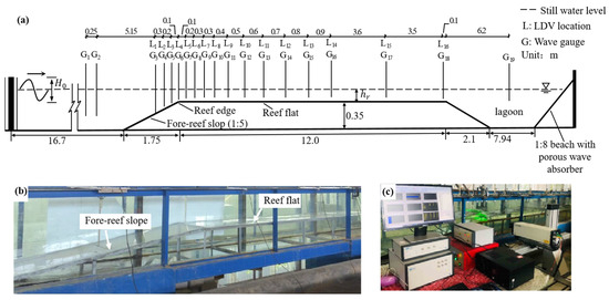
Figure 1.
(a) A sketch of the laboratory setup; (b) the physical reef model; (c) the LDV instrument.
2.2. Instruments and Test Scenario
As shown in Figure 1a, 19 resistance-type wave gauges, denoted as G1–G19, were deployed across the wave flume to monitor the wave process. G1 and G2 were placed offshore to measure the incident waves. G3–G18 were located along the reef profile with more gauges set in the reef surf zone around the reef edge. G19 was put in the lagoon. Waves were recorded with a sample frequency of 50 Hz. To measure the detailed wave-driven current, measurements using a Laser Doppler velocimeter (LDV), which non-intrusively obtains the two-dimensional flow components at a single point, were obtained recursively along the depth of the flow (Figure 1c). This instrument outperforms the commonly used acoustic Doppler velocimeter (ADV) due to its accuracy and flexibility on the shallow reef; see Yao et al. [4] for a comparison of the flow measurements between the two instruments. The instantaneous velocities were recorded in both the streamwise and vertical directions at the maximum data rate achievable by the instrument. The variation in the vertical velocity profile was sampled at 16 points (denoted as L1–L16) along the longitudinal centerline of reef profile (Figure 1a). More sampling points were also arranged in the surf zone close to the reef edge. At each position, velocities from the wave trough to the seabed were monitored at 5 mm intervals using the LDV with the help of an automated supporting frame. After completing the measurement at a cross-shore position, the instrument was shifted to the next position in the same wave run. To reach a quasi-steady hydrodynamic state in the flume, both measurements of wave and flow were conducted after running the wave generator for more than half an hour. The sampling duration was set to 90 s for both waves and currents, except for locations near the incipient breaking point. Air bubble effects on the measurements were significant for those positions; thus, the recording duration was extended to 180 s.
A single regular wave scenario (, , and , where and are the incident deep-water wave height and wave period and is the reef flat submergence) was tested in this study, and it generated a classical plunging breaker on the designed fringing reef model. Note that the experimental settings in this study were also improved from those of Yao et al. [3] in view of a flow measurement area extending to the entire reef flat (they only measured the flow around the surf zone) as well as a larger incident wave height (their was 0.12 m).
3. Numerical Setup
3.1. Governing Equations
In the present study, we utilized the widely adopted open source computational fluid dynamics library OpenFOAM® to establish our numerical wave flume. Specifically, we employed the Reynolds Averaged Navier–Stokes equations with an interface-compression Volume of Fluid (VOF) method to track the free surface. The governing equations and free-surface-tracking techniques are well known and, therefore, are omitted here for concision. Interested readers are referred to relevant prior publications (i.e., ref. [28]) for details. Here, we mainly focus on the turbulence closure and its special treatments to improve the stability.
For turbulence closure, we use the following k-ω SST turbulence model [29].
with and being the velocity and spatial coordinate components, respectively; being the kinematic viscosity of water; being the turbulent kinematic viscosity; being a production term of the turbulent kinetic energy; and being the specific dissipation rate; being the mean strain rate of flow; being a coefficient related to the production of ; and and being the blending function coefficients [30]. The values of the parameters , , and were determined according to the mixture of an inner constant () and an outer constant ():
In this study, we used the default values for the model parameters, which are , , , , , , , , , and .
In order to suppress the turbulence over-production associated with waves while maintaining the Boussinesq approximation, a turbulence correction scheme was used following that of Larsen and Fuhrman [25]. A limiter was introduced to when evaluating , using Equation (5):
with being a stress-limiting coefficient. , with being the mean rotation rate and being a production coefficient defined as
3.2. Numerical Wave Flume
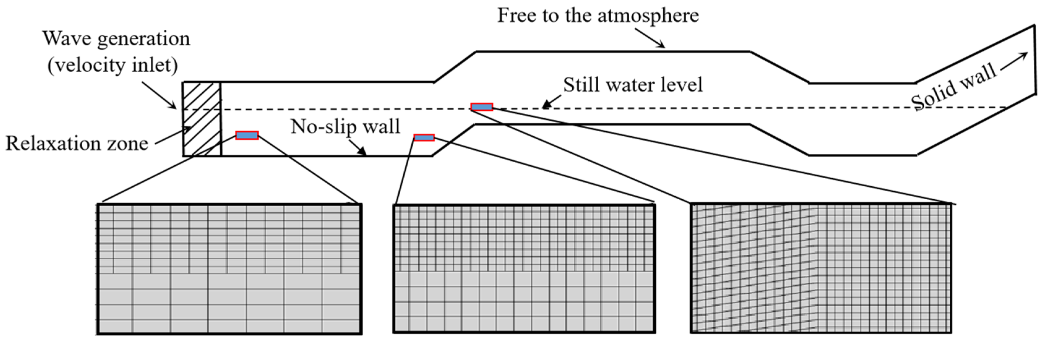
The numerical wave flume was established to fully reproduce the laboratory conditions (Figure 2). The top boundary was set to be atmospheric, while both sides were set to be “empty” boundaries in OpenFOAM® considering the 2DV reef configuration in this study. Both the bottom boundary and the reef profile were treated as no-slip solid walls for which the wall functions were introduced for and using the approach proposed by Menter and Esch [31]. Design waves were generated at the left boundary using the relaxation zone method, as implemented in the waves2Foam package [32] included in OpenFOAM®. Linear wave theory was employed to produce the designed regular waves. The relaxation zone was set to be at the left end of the flume, with its width being twice the design wave length in this study.
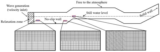
Figure 2.
Boundary conditions and mesh settings in the numerical wave flume.
To save on computational cost, simple unstructured grids with only one layer of 4 mm in the alongshore () direction were used in the numerical flume. In the cross-shore () direction, the grid size slowly reduced from 20 mm to 8 mm from the left boundary of wave generation to the toe of the fore-reef slope. Behind that, the grid size was kept at a constant value of = 2 mm along the reef until to the right boundary. Meanwhile, a constant grid size of = 8 mm was assigned in the vertical () direction for the entire domain, but the grid refinement in a region 10 cm both above and below the still water level was also performed by decreasing to 2 mm. The final mesh had about 2.43 million hexagonal cells. We found via pilot tests that, using the present grid setup, an in-simulation duration of 100 wave cycles is usually sufficient to generate reliable results (see also Yao et al. [3] for a grid size convergence test). An adjustable time step setting with a Courant number of 0.4 was used in all simulations. A single simulation case took about 36 h running parallel on a small computing cluster with 100 CPUs (Intel Xeon 8173M, 2.0 GHz).
4. Experimental Results
4.1. Wave Height and Mean Water Level across the Reef
As shown in Figure 3a, wave height () rises when waves shoal over the fore-reef slope; it then reaches its peak value near the reef edge, where the incipient wave breaking happens. After that, decreases significantly in the surf zone around the outer reef flat. Behind the surf zone on the inner reef flat, organized waves re-form, and they keep on propagating shoreward and eventually enter the lagoon. A gradual wave height decay is observed due possibly to the bottom friction.
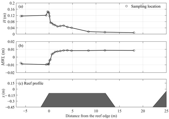
Figure 3.
Cross-shore distribution of the experimental: (a) wave height (); (b) mean water level (MWL); and (c) the reef profile, shown for convenience. indicates the still-water level (, , and ).
Regarding the mean water level (MWL) shown in Figure 3b, the set-down (i.e., MWL < 0) on the seaside of the reef profile is attributed to mass balance within a closed domain: the water pileup on a reef should be compensated by the water loss at the offshore side as a set-down. Meanwhile, MWL declines continuously across the fore-reef slope because of the shoaling process. On the outer reef flat in the surf zone, a notable growth in MWL associated with wave breaking can be found. The maximum MWL appears at the endpoint of surf zone as wave setup (i.e., MWL > 0). After that, the wave setup becomes almost constant on the reef flat. Overall, the above findings about and MWL are consistent with the existing laboratory experiments for fringing reefs [33,34].
4.2. The Vertical Variations in Cross-Reef Mean Flows along the Reef Profile
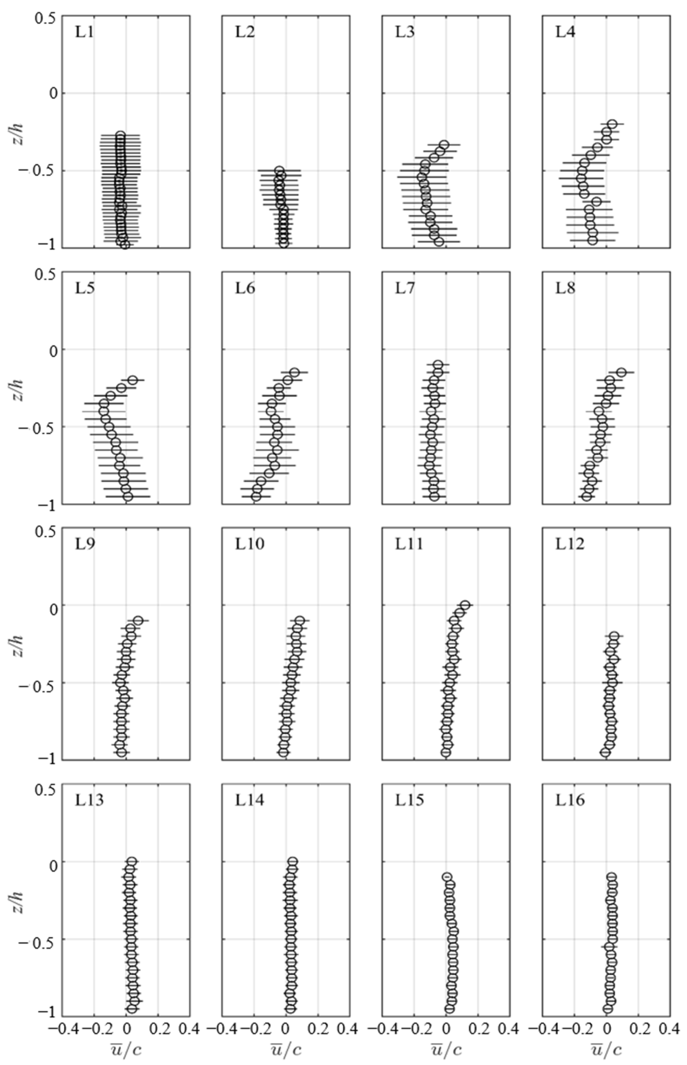
Next, we examine the distributions of cross-reef mean velocity () along the water depth from the 16 flow measurement locations (Figure 4). The mean flow and its fluctuation were obtained based on the ensemble average and the standard deviation of the wave phase-averaged velocities over the last 20 measured wave cycles, respectively, and the phase-averaged velocity was estimated by taking averages of the measurements within each wave cycle. The sampling fluctuations (represented by error bars) were found to be larger around the breaking point between locations L2 and L5, where the effect of air bubble on flow measurement was notable (Figure 4).
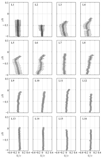
Figure 4.
Vertical variations in measured normalized mean cross-reef currents () at the velocity measurement positions (L1–L16) along the reef profile. indicates the still-water level, error bars denote the measurement fluctuations, represents the local shallow wave speed, and positive/negative values of indicate the onshore/offshore directed currents. (, , and ).
For the subsequent analysis in this section, we normalize with , where is the shallow water wave phase celerity, is the gravity acceleration, and is the local water depth. Figure 4 indicates that, overall, the vertical structure of the mean cross-shore current across the fringing reef profile is identical to that measured for a beach profile under a typical plunging breaker [35]. The mean flows () on the fore-reef slope associated with the shoaling waves (L1–L2) are slightly offshore-directed, and their magnitudes rise almost linearly from the seabed to the wave trough. L3–L5 are located in the outer surf zone between the incipient breaking point and the plunging point. It can be observed that the undertow current starts to increase from the bottom, moves upwards to a region around the wave trough, and then turns toward the shoreward current due to wave mass transport. For locations L6–L12 in the inner surf zone, where breaking waves travel onshore as moving bores, the vertical variation in undertow reverses, with the peak undertow being found around the seabed and onshore mass transport being observed near the wave trough. The maximum undertow can be seen near the seabed at L6, which is about . Such a flow regime is identical to that measured on a similar fringing reef configuration [3], in that the depth-controlled mass balance requires that the wave-driven shoreward transport be balanced by the undertow below the wave trough. For the locations behind the surf zone (L13–L16) on the remaining reef flat, there are almost no cross-reef wave-induced mean flows. A more detailed mean flow pattern including the area between wave tough and wave crest will be analyzed based on numerical data in Section 6.1.
5. Numerical Model Verification
5.1. The Time Series of Free Surface Elevations and Mid-Depth Velocities
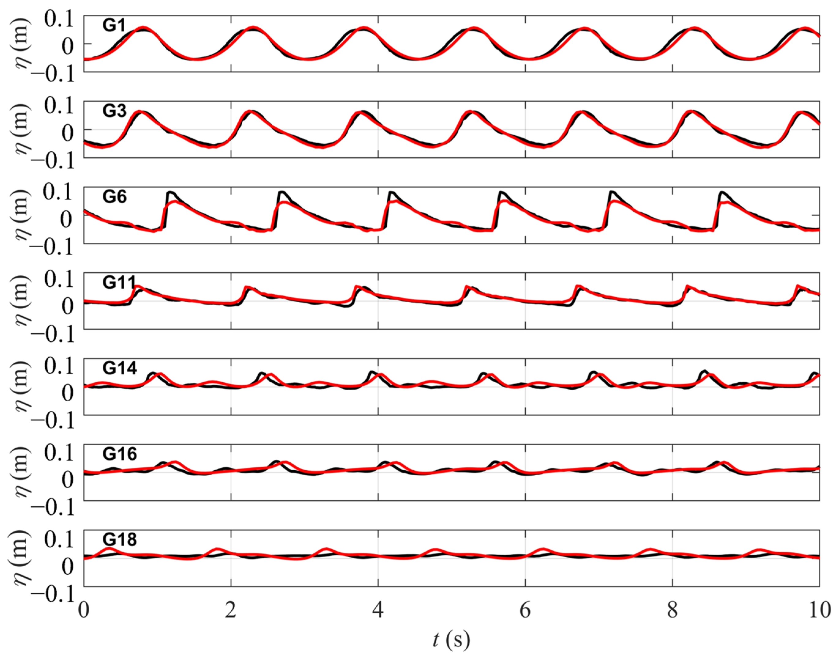
Figure 5 shows comparisons between the simulations and measurements of a time series of free surface elevations () from seven selected wave sampling positions. Satisfactory predictions for can be seen for most positions, including those for offshore wave propagation (G1), fore-reef slope wave shoaling (G3), and outer reef flat wave breaking (G6 and G11). The adopted numerical approach also reasonably reproduces transmitted waves near the middle reef flat (G14 and G16) as well as the multiple peaks of wave profile due to the higher harmonics generated on the reef profile [36]. However, there is slight over-prediction of wave crest for the location near the lagoon (G18).
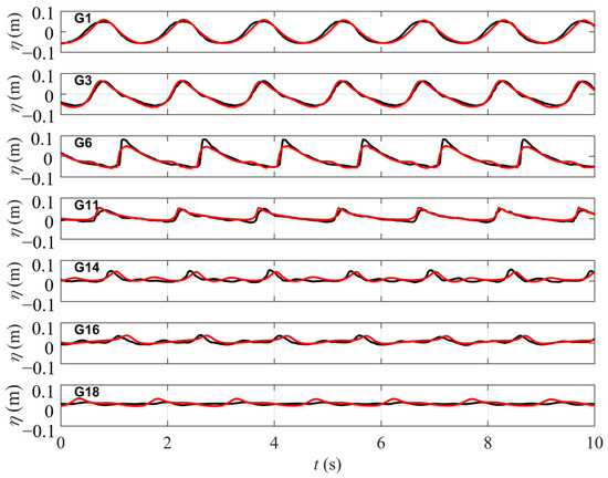
Figure 5.
Comparison between numerical and experimental time series of free surface elevations at seven representative sampling positions. Black lines denote measurements; red lines denote simulations (, , and ).
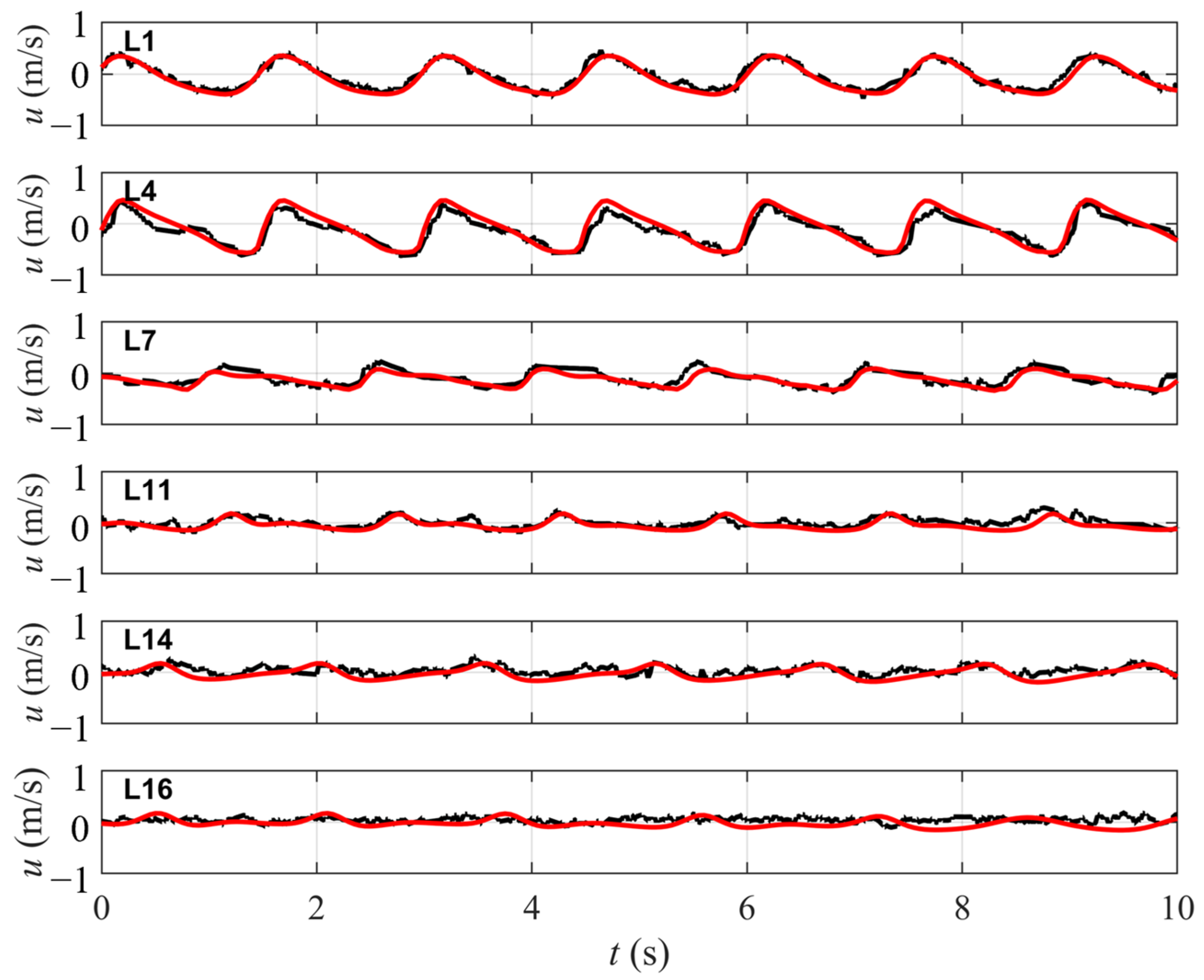
The experimental and numerical time series of cross-shore velocities () obtained from the mid-depth of six selective sampling positions are then compared (Figure 6). Good agreements for both in the shoaling region on the fore-reef slope (L1) and around the breaking point near the reef edge (L4) can be found. The numerical simulation can also satisfactorily predict the velocities from both L7 and L11 in the surf zone, although the currents from those positions are less organized as a result of the wave-breaking-induced turbulence. At L14 and L16, where wave breaking ceases, flows are more stable under the re-formed waves and the model predictions still have reasonable agreement with the experiments.
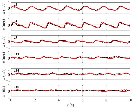
Figure 6.
Comparison between numerical and experimental mid-depth velocities at six representative sampling positions. Black lines denote measurements; red lines denote simulations (, , and ).
5.2. The Cross-Reef Envolutions of Wave Height and MWL
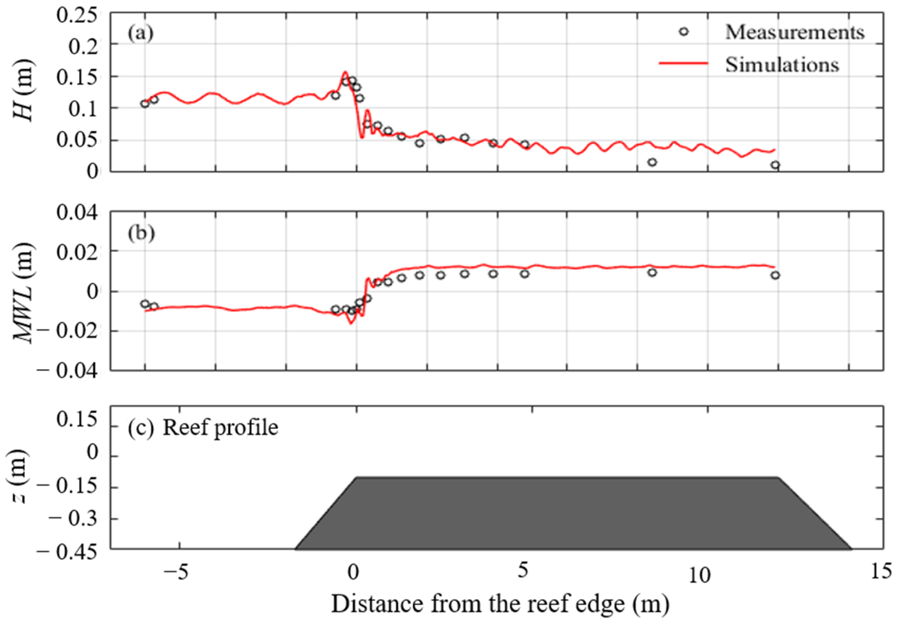
Subsequently, the cross-reef distributions of both the numerical and experimental wave height () and MWL are compared (Figure 7). In general, the numerical approach can satisfactorily predict a rise in on the fore-reef slope, which is clearly due to wave shoaling. A rapid drop in due to wave breaking around the reef edge as well as a slow decline in it on the reef flat are also observed. However, the transmitted wave height on the inner reef flat is over-predicted; this is attributed to the porous wave absorber on the final beach in the experiments, which is not addressed in the numerical model. The fluctuation in distribution across the reef is due to the partial standing waves caused by the reflected waves from the fore-reef slope and/or the final beach. The numerical model also reasonably reproduces a slow decline in MWL, known as a wave set-down over the fore-reef slope; a sharp increase in MWL in the surf zone near the reef edge; and a nearly constant wave-generated setup across the reef flat.
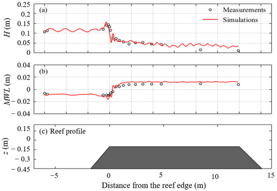
Figure 7.
Comparison between numerical and experimental results: (a) wave height () and (b) mean water level (MWL) along the reef profile. Subfigure (c) shows the reef profile for convenience. (, , and ).
5.3. The Vertical Profile of Cross-Reef Mean Flow
The aforementioned experimental work cannot record the velocity above the wave trough due to instrument limitations. To overcome this deficiency, we use the numerical results, which can provide mean current distribution both below and above the wave trough. The computed and measured vertical cross-reef mean flow profiles are compared in Figure 8.
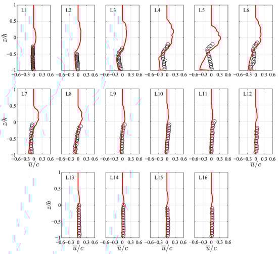
Figure 8.
Comparison between numerical and experimental vertical variations in measured normalized mean cross-reef current () at the velocity measurement positions L1–L16 along the reef profile. indicates the still water level. represents the local shallow wave speed, and positive/negative values of indicate the onshore/offshore directed currents (, , and ). Circles denote measurements; red lines denote simulations.
The model predictions for the depth variation in mean current under shoaling waves over the fore-reef slope (L1–L3) appear to be satisfactory. Wave breaking is energetic in the outer surf zone around the reef edge (L4–L5), and the mean current profiles are captured reasonably at those locations, albeit with some overestimation of the undertow current appearing, which is possibly associated with the overestimation of the breaker roller speed close to the water–air interface. Such overestimation is also observed in other numerical studies of wave breaking using OpenFOAM with interface compression VOF techniques (see, for example, Jacobsen et al. [32]). The model performances for those locations in the inner surf zone (L6–L12) are reasonably good. Finally, the model also satisfactorily reproduces the mean currents at those locations behind the surf zone (L13–L16), although they are very small. Existing numerical investigation on wave-driven flow over the fringing reef, such as that in Yao et al. [3], using a buoyancy-modified k-ω SST turbulence closure also found that the undertow profiles in the surf zone were overestimated. Such over-prediction is largely suppressed based on the adopted model configuration, particularly in the inner surf zone.
6. Numerical Model Application
6.1. Mean Current Field along the Reef Profile
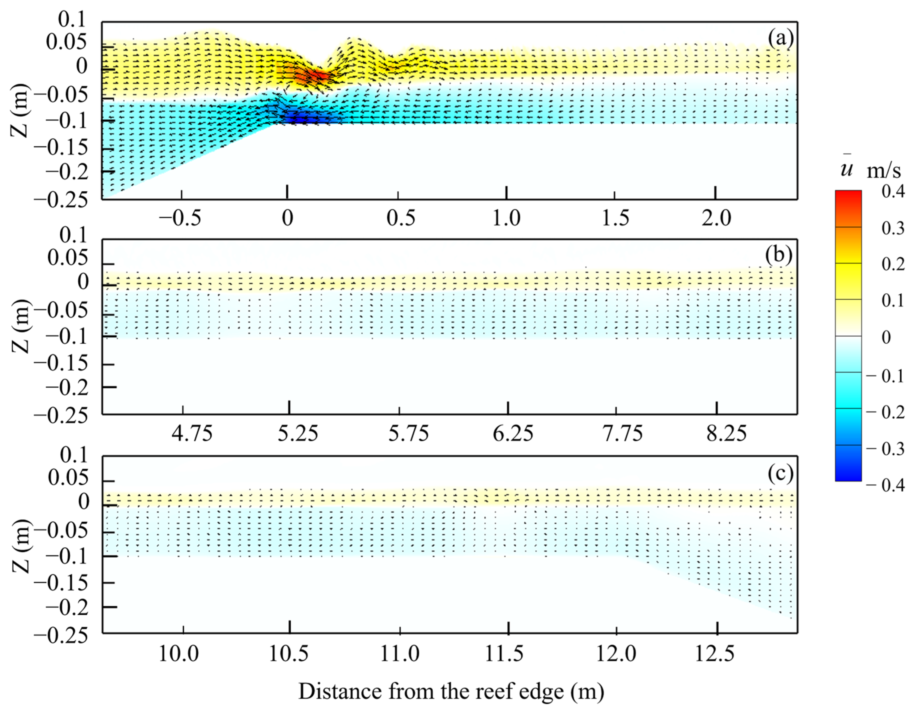
The 2DV mean cross-shore flow fields at the outer, central, and inner reef flats are shown in Figure 9a–c, respectively. The dominant flow pattern is due to the cross-shore mass balance: the wave-generated onshore mass transport above the wave trough should be offset by the offshore-directed flow (undertow) underneath, resulting in 2DV circulation. Such circulation appears to be strongest in the inner surf zone around the reef edge, where wave breaking is energetic. In the rest of the reef flat after the surf zone, both the onshore mass transport and the seaward undertow are very weak. Finally, we remark that the present 2DV reef configuration can mimic fringing reefs where no rip channel is present or where the rip channel is far away and thus the lateral (alongshore) effect is weak. An example of these scenarios can be found for a fringing reef flat at Guam during the tropical storm Man-Yi [37]. Previous theoretical considerations [38] have recognized both the magnitude and direction of the near-bed mean flow in determining the reef-top hydrodynamics through the bottom friction based on the cross-shore momentum balance. Our findings hence show a necessity in using a Navier–Stokes equation-based approach to resolve the vertical variation in the cross-reef flow for fully understanding the underlying mechanism.
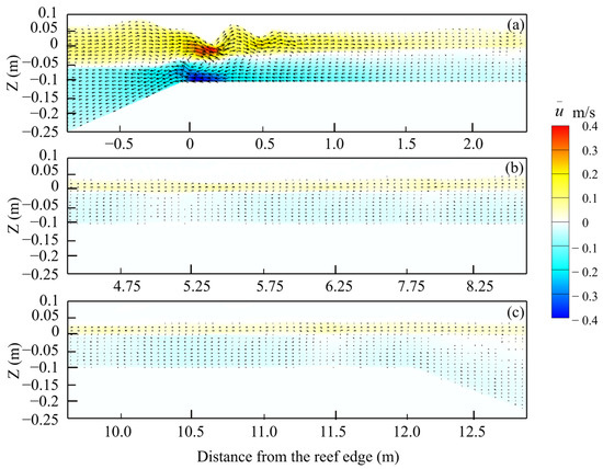
Figure 9.
The computed 2DV evolution of cross-reef mean flow () around (a) the outer, (b) the central. and (c) the inner reef flats. indicates the still-water level (, , and ).
6.2. TKE and Reynolds Shear Stress along the Reef Profile
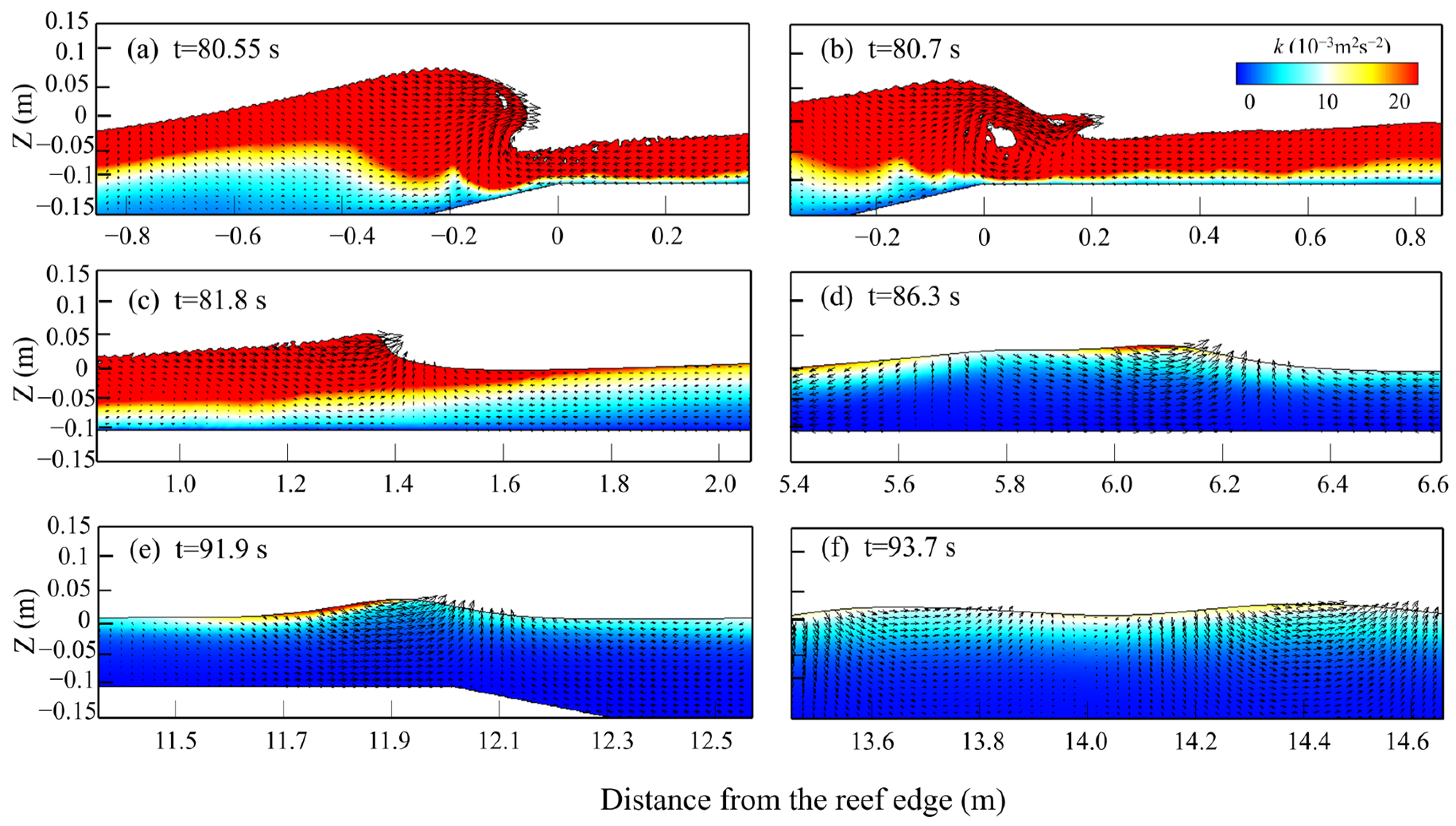
Another advantage of the present numerical approach is its capability to provide the flow turbulence characteristics along the reef profile, which is important to the sediment process across the reef. Based on the aforementioned wave scenario, Figure 10 shows the simulated 2DV TKE distribution associated with the wave propagation in six selected regions across the reef.

Figure 10.
The computed 2DV evolution of the TKE () over various regions along the reef. indicates the still-water level, and represents the wave-travelling time from generation (, , and ).
Close to the reef edge where wave breaking occurs (Figure 10a), a stronger is observed under the wave crest. After wave breaking occurs, larger values of can be seen around the upper water layer; this could be associated with the moving bore (Figure 10b). Both the magnitude and the extent of drop gradually as the moving bore decays all the way on the outer reef flat (Figure 10c). Consequently, significant values of are only notable near the free surface as the transmitted wave re-forms near the central reef flat (Figure 10d) and moves onto the inner reef flat (Figure 10e). When waves travel further into the lagoon (Figure 10f), turns out to be very small.
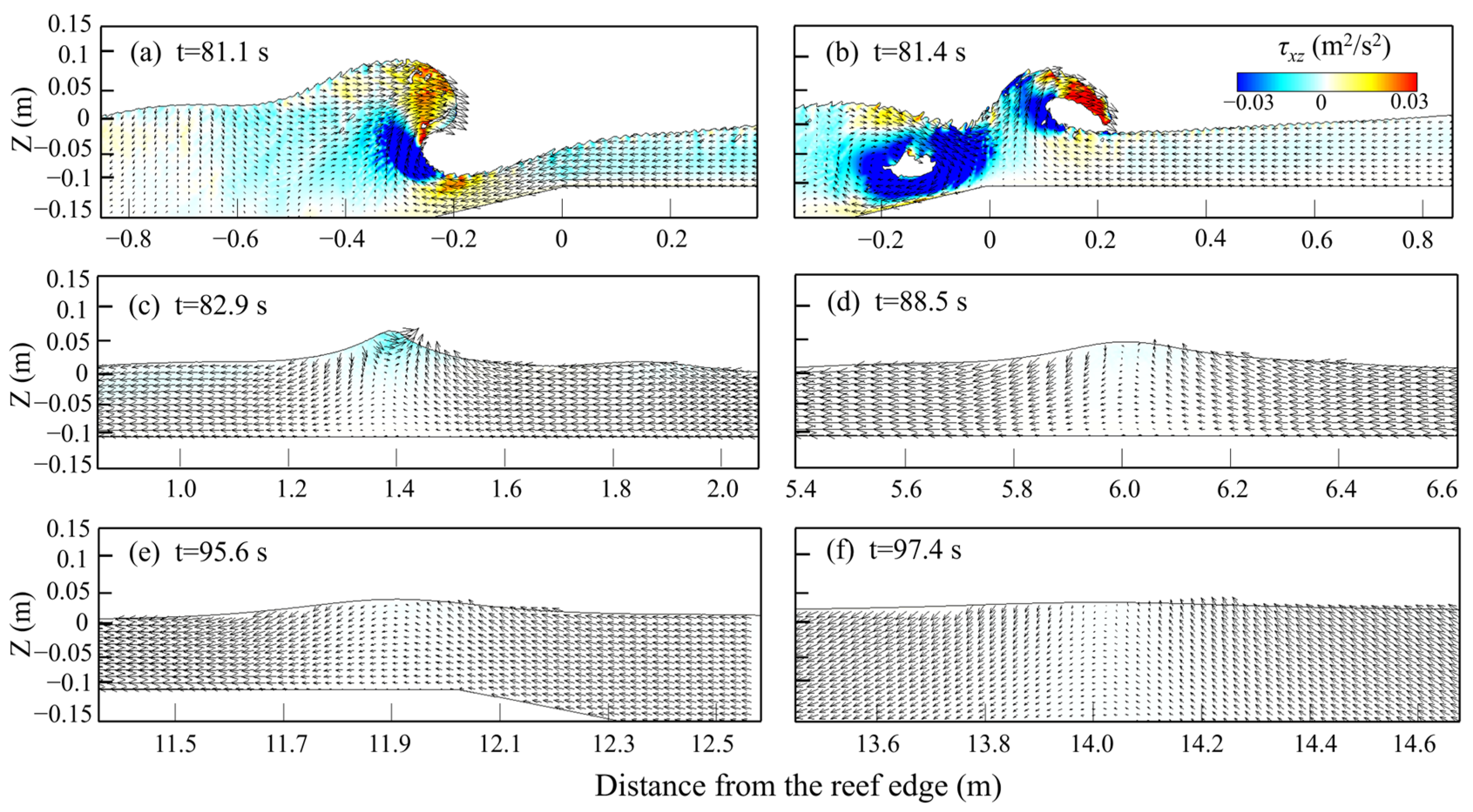
Besides TKE, Reynolds stress is another commonly used variable to characterize the turbulence. It represents the rate of mean momentum transferred by turbulent fluctuations to mean flow. Similar to the analysis of TKE above, the predicted 2DV distribution of the Reynolds shear stress, , over selected reef regions are displayed in Figure 11. The normal Reynolds stresses can be derived based on the TKE; hence, they are not presented here.
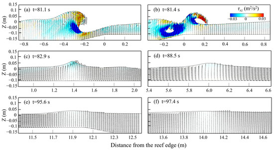
Figure 11.
The computed 2DV evolution of the Reynolds shear stress () over various regions along the reef. indicates the still water level, and represents the wave-travelling time from generation (, , and ).
In the wave scenario shown in Figure 11, wave breaking initiates around the reef edge, with a positive around the wave crest tip and a negative around the toe of wave crest (Figure 11a). As a breaking wave plunges on the outer reef flat, a region with negative extends along the entire water depth (Figure 11b), suggesting that strong momentum has transferred from the mean current to the turbulence fluctuations. The value of under the moving bore drops rapidly at the outer reef flat, with only negative occurring around the bore (Figure 11c). After a breaking wave disappears, the magnitude of decreases significantly, with almost zero around the re-formed wave at both the central and inner reef flats (Figure 11d,f).
7. Conclusions
In this paper, detailed flow measurements along the water depth were conducted in a wave flume using an advanced LDV system to better characterize the wave-induced flow along a fringing reef associated with a plunging breaker. The experimental results indicated that both the re-formed wave height and the wave-induced setup in the inner reef flat were nearly constant, which is commonly observed for fringing reefs. Overall, the vertical variation in mean cross-reef current is identical to that measured for a beach profile under a typical plunging breaker. The mean flows are onshore above the wave trough due to the wave-driven mass transport, while they are predominantly offshore-directed below the wave trough in the form of undertow.
A numerical wave flume was developed in this paper via the open source CFD toolbox OpenFOAM®. A modified k-ω SST turbulence closure with enhanced numerical stability in wave modeling was adopted in tandem with the standard RANS governing equation. The adopted model was first verified with both wave and flow laboratory measurements. It was then applied to analyze the cross-reef distributions of mean current field, TKE, and Reynolds shear stress. Model applications indicate that the wave-driven onshore mass transport above the wave trough can be compensated by the undertow underneath, resulting in vertical circulation, particularly around the surf zone. Both TKE and Reynolds shear stress are found to be significant around the plunging point in the reef surf zone, but both their magnitudes and extents are reduced as breaking waves travel further inland on the reef flat.
The laboratory data reported in our study can potentially be used to verify other analytical and numerical approaches proposed to model wave processes in a fringing reef configuration. This study also proves that RANS-based CFD models, when coupled with a delicate choice of turbulence closure, is a good choice for resolving the vertical variation in mean flow as well as the turbulence characteristics over coral reefs, at least at the laboratory scale.
Author Contributions
Conceptualization, T.Y. and Y.Y.; methodology, Y.Y.; software, C.X.; validation, T.Y. and Z.L.; formal analysis, T.Y.; investigation, T.Y.; resources, C.X.; data curation, Z.L.; writing—original draft preparation, T.Y.; writing—review and editing, Y.Y.; visualization, Y.Y.; supervision, Y.Y.; project administration, Y.Y.; funding acquisition, Y.Y. All authors have read and agreed to the published version of the manuscript.
Funding
This work is sponsored by the National Key Research and Development Program of China (grant No. 2021YFC3100500), the National Natural Science Foundation of China (grant No. 51979013), and the Science and Technology Innovation Plan Project of Hunan Province (grant No. 2022RC3043).
Institutional Review Board Statement
Not applicable.
Informed Consent Statement
Not applicable.
Data Availability Statement
Not applicable.
Conflicts of Interest
The authors declare no conflict of interest.
References
- Lowe, R.J.; Falter, J.L. Oceanic forcing of coral reefs. Annu. Rev. Mar. Sci. 2015, 7, 43–66. [Google Scholar] [CrossRef] [PubMed]
- Rijnsdorp, D.P.; Buckley, M.L.; da Silva, R.F.; Cuttler, M.V.W.; Hansen, J.E.; Lowe, R.J.; Green, R.H.; Storlazzi, C.D. A numerical study of wave-driven mean flows and setup dynamics at a coral reef-lagoon system. J. Geophys. Res. Ocean. 2021, 126, e2020JC016811. [Google Scholar] [CrossRef]
- Yao, Y.; Liu, Y.C.; Chen, L.; Deng, Z.Z.; Jiang, C.B. Study on the wave-driven current around the surf zone over fringing reefs. Ocean Eng. 2020, 198, 106968. [Google Scholar] [CrossRef]
- Yao, Y.; Li, Z.Z.; Xu, C.H.; Jiang, C.B. A study of wave-driven flow characteristics across a reef under the effect of tidal current. Appl. Ocean Res. 2023, 130, 103430. [Google Scholar] [CrossRef]
- Clark, S.J.; Becker, J.M.; Merrifield, M.A.; Behrens, J. The influence of a cross-reef channel on the wave-driven setup and circulation at Ipan, Guam. J. Geophys. Res. Ocean. 2020, 125, e2019JC015722. [Google Scholar] [CrossRef]
- Hench, J.L.; Leichter, J.J.; Monismith, S.G. Episodic circulation and exchange in a wave-driven coral reef and lagoon system. Limnol. Oceanogr. 2008, 53, 2681–2694. [Google Scholar] [CrossRef]
- Lowe, R.J.; Falter, J.L.; Monismith, S.G.; Atkinson, M.J. Wave-driven circulation of a coastal reef-lagoon system. J. Phys. Oceanogr. 2009, 39, 873–893. [Google Scholar] [CrossRef]
- Sous, D.; Chevalier, C.; Devenon, J.L.; Blanchot, J.; Pagano, M. Circulation patterns in a channel reef-lagoon system, Ouano lagoon, New Caledonia. Estuar. Coast. Shelf Sci. 2017, 196, 315–330. [Google Scholar] [CrossRef]
- Gourlay, M.R. Wave set-up on coral reefs. 1. Set-up and wave generated flow on an idealised two dimensional reef. Coast. Eng. 1996, 27, 161–193. [Google Scholar] [CrossRef]
- Yao, Y.; Huang, Z.H.; He, W.R.; Monismith, S.G. Wave-induced setup and wave-driven current over Quasi-2DH reef-lagoon-channel systems. Coast. Eng. 2018, 138, 113–125. [Google Scholar] [CrossRef]
- Zheng, J.H.; Yao, Y.; Chen, S.G.; Chen, S.B.; Zhang, Q.M. Laboratory study on wave-induced setup and wave-driven current in a 2DH reef-lagoon-channel system. Coast. Eng. 2020, 162, 103772. [Google Scholar] [CrossRef]
- Yao, Y.; Becker, J.M.; Ford, M.R.; Merrifield, M.A. Modeling wave processes over fringing reefs with an excavation pit. Coast. Eng. 2016, 109, 9–19. [Google Scholar] [CrossRef]
- Yao, Y.; Zhang, Q.M.; Chen, S.G.; Tang, Z.J. Effects of reef morphology variations on wave processes over fringing reefs. Appl. Ocean Res. 2019, 82, 52–62. [Google Scholar] [CrossRef]
- Ning, Y.; Liu, W.J.; Zhao, X.Z.; Zhang, Y.; Sun, Z.L. Study of irregular wave runup over fringing reefs based on a shock-capturing Boussinesq model. Appl. Ocean Res. 2019, 84, 216–224. [Google Scholar] [CrossRef]
- Su, S.F.; Ma, G.; Tsu, T.W. Boussinesq modeling of spatial variability of infragravity waves on fringing reefs. Ocean Eng. 2015, 101, 78–92. [Google Scholar] [CrossRef]
- Liu, Y.; Liao, Z.; Fang, K.; Li, S. Uncertainty of wave runup prediction on coral reef-fringed coasts using SWASH model. Ocean Eng. 2021, 242, 110094. [Google Scholar] [CrossRef]
- Ma, G.; Su, S.F.; Liu, S.; Chu, J.C. Numerical simulation of infragravity waves in fringing reefs using a shock-capturing non-hydrostatic model. Ocean Eng. 2014, 85, 54–64. [Google Scholar] [CrossRef]
- Shi, J.; Zhang, C.; Zheng, J.H.; Tong, C.F.; Wang, P.; Chen, S.G. Modelling wave breaking across coral reefs using a non-hydrostatic model. J. Coast. Res. 2018, 85, 501–505. [Google Scholar] [CrossRef]
- Van Dongeren, A.; Lowe, R.; Pomeroy, A.; Trang, D.M.; Roelvink, D.; Symonds, G.; Ranasinghe, R. Numerical modeling of low-frequency wave dynamics over a fringing coral reef. Coast. Eng. 2013, 73, 178–190. [Google Scholar] [CrossRef]
- Lashley, C.H.; Roelvink, D.; Van Dongeren, A.; Buckley, M.L.; Lowe, R.J. Nonhydrostatic and surfbeat model predictions of extreme wave run-up in fringing reef environments. Coast. Eng. 2018, 137, 11–27. [Google Scholar] [CrossRef]
- Franklin, G.; Mariño-Tapia, I.; Torres-Freyermuth, A. Effects of reef roughness on wave setup and surf zone currents. J. Coast. Res. 2013, 118, 2005–2010. [Google Scholar] [CrossRef]
- Li, J.X.; Zang, J.; Liu, S.X.; Jia, W.; Chen, Q. Numerical investigation of wave propagation and transformation over a submerged reef. Coast. Eng. J. 2019, 61, 363–379. [Google Scholar] [CrossRef]
- Osorio-Cano, J.D.; Alcérreca-Huerta, J.C.; Osorio, A.F.; Oumeraci, H. CFD modelling of wave damping over a fringing reef in the Colombian Caribbean. Coral Reefs. 2018, 37, 1093–1108. [Google Scholar] [CrossRef]
- Devolder, B.; Troch, P.; Rauwoens, P. Performance of a buoyancy-modified, k-ω and, k-ω SST turbulence model for simulating wave breaking under regular waves using OpenFOAM®. Coast. Eng. 2018, 138, 49–65. [Google Scholar] [CrossRef]
- Larsen, B.E.; Fuhrman, D.R. On the over-production of turbulence beneath surface waves in Reynolds-averaged Navier–Stokes models. J. Fluid. Mech. 2018, 853, 419–460. [Google Scholar] [CrossRef]
- Becker, J.M.; Merrifield, M.A.; Ford, M. Water level effects on breaking wave setup for Pacific Island fringing reefs. J. Geophys. Res. Ocean. 2014, 119, 914–932. [Google Scholar] [CrossRef]
- Lowe, R.J.; Falter, J.L.; Bandet, M.D.; Pawlak, G.; Atkinson, M.J. Spectral wave dissipation over a barrier reef. J. Geophys. Res. 2015, 110, 169–189. [Google Scholar] [CrossRef]
- OpenFOAM® User Guide, 2013. The OpenFOAM Foundation. Available online: http://www.openfoam.org (accessed on 20 July 2022).
- Menter, F.; Ferreira, J.C.; Esch, T.; Konno, B. The SST turbulence model with improved wall treatment for heat transfer predictions in gas turbines. In Proceedings of the International Gas Turbine Congress 2003, Tokyo, Japan, 2–7 November 2003. [Google Scholar]
- Menter, F.R. Two-equation eddy-viscosity turbulence models for engineering applications. AIAA J. 1994, 32, 1598–1605. [Google Scholar] [CrossRef]
- Menter, F.; Esch, T. Elements of industrial heat transfer predictions. In Proceedings of the 16th Brazilian Congress of Mechanical Engineering (XVI Congresso Brasileiro de Engenharia Mecânica), Uberlândia, Brazil, 26–30 November 2001; COBEM 2001, Invited Lectures. Volume 20, p. 117e27. [Google Scholar]
- Jacobsen, N.G.; Fuhrman, D.R.; Fredsøe, J. A Wave Generation Toolbox for the Open-Source CFD Library: OpenFoam®. Int. J. Numer. Methods Fluids 2012, 70, 1073–1088. [Google Scholar] [CrossRef]
- Buckley, M.L.; Lowe, R.J.; Hansen, J.E.; Van Dongeren, A.R. Dynamics of wave setup over a steeply sloping fringing reef. J. Phys. Oceanogr. 2015, 45, 3005–3023. [Google Scholar] [CrossRef]
- Demirbilek, Z.; Nwogu, O.G.; Ward, D.L. Laboratory Study of Wind Effect on Runup over Fringing Reefs, Report 1: Data Report; Coastal and Hydraulics Laboratory Technical Report ERDC/CHL-TR-07-4; U.S. Army Engineer Research and Development Center: Vicksburg, MS, USA, 2007. [Google Scholar]
- Ting, F.C.K.; Kirby, J.T. Observation of undertow and turbulence in a laboratory surf zone. Coast. Eng. 1994, 24, 51–80. [Google Scholar] [CrossRef]
- Yao, Y.; Chen, X.J.; Xu, C.H.; Jia, M.J.; Jiang, C.B. Numerical modelling of wave transformation and runup over rough fringing reefs using VARANS equations. Appl. Ocean Res. 2022, 118, 102952. [Google Scholar] [CrossRef]
- Vetter, O.; Becker, J.M.; Merrifield, M.A.; Péquignet, A.C.; Aucan, J.; Boc, S.J.; Pollock, C.E. Wave setup over a Pacific Island fringing reef. J. Geophys. Res. 2010, 115, C12066. [Google Scholar] [CrossRef]
- Buckley, M.L.; Lowe, R.J.; Hansen, J.E.; van Dongeren, A.R. Wave setup over a fringing reef with large bottom roughness. J. Phys. Oceanogr. 2016, 46, 2317–2333. [Google Scholar] [CrossRef]


Disclaimer/Publisher’s Note: The statements, opinions and data contained in all publications are solely those of the individual author(s) and contributor(s) and not of MDPI and/or the editor(s). MDPI and/or the editor(s) disclaim responsibility for any injury to people or property resulting from any ideas, methods, instructions or products referred to in the content. |
© 2023 by the authors. Licensee MDPI, Basel, Switzerland. This article is an open access article distributed under the terms and conditions of the Creative Commons Attribution (CC BY) license (https://creativecommons.org/licenses/by/4.0/).