Optimal Smoothing of the Wind–Wave Spectrum Based on the Confidence-Interval Trade-Off

Abstract

In this study, a smoothing method was applied to improve the accuracy of peak wave period estimation using water surface elevation data collected from two oceanographic and meteorological observation towers situated on the western coast of the Korean Peninsula. The effectiveness of the smoothing method was validated by assessing the surface elevation variance and total wave energy. Subsequently, we examined the impact of the smoothing application. The results of our analysis revealed a reduction of approximately 27% in comparison to the confidence interval of the initially estimated spectrum upon applying the smoothing method. Furthermore, a slight variation of approximately 1–2 s was observed between the peak wave period calculated from the estimated spectrum and that obtained through the smoothing process. Utilizing statistical methods to determine the optimal smoothing parameter count, we observed an increasing trend as the range of significant wave heights decreased.

1. Introduction

The key parameters for distinguishing irregular oceanographic characteristics are wave height and period, which are typically analyzed using water surface elevation data. Given that wave height and period are dynamic and location-dependent, it is essential to comprehend diverse wave attributes from an engineering standpoint [1]. Recently, due to advancements in oceanographic observation systems, obtaining wave information conducive to varied analyses has become more accessible, elevating the significance of wave observation data. Approaches for analyzing irregular wave characteristics encompass the following: (1) the wave-train method, involving a direct analysis of water surface elevation data in the time domain, and (2) the analysis of irregular wave spectra, which involves assessing spectra in the frequency domain [2,3,4]. The wave-train analysis method, prominently employed in the design of marine structures such as breakwaters, identifies individual waves and computes wave height and period as they traverse a reference point. Stansell et al. (2002) [5] and Mazeika and Draudviliene (2010) [6] investigated wave height variation patterns across observation time intervals using the wave-train analysis approach. Nishi et al. (1997) [7] and Choi et al. (2017) [8] derived wave parameters through a wave-train analysis method employing the zero-crossing technique. However, when employing the wave-train analysis method for wave height estimation, there is a possibility of underestimation compared to the spectrum analysis method, primarily because the observation interval often deviates from successive waveform peak and trough points [9].

Contrarily, the spectrum analysis method, a fundamental approach to computing pivotal wave characteristics, evaluates the energy distribution of waves through a frequency function. It also determines the period and corresponding area related to the frequency featuring the highest energy density [10]. This method presumes that the ocean’s numerous waves are composed of various sine waves with distinct amplitudes and frequencies. In contrast, Pierson and Marks (1952) [11] and Casas Prat (2008) [12] introduced a wave spectrum analysis method applicable for investigating spectral distribution estimation within a designated area, conducted an extreme value analysis, and developed numerical models for wave transformation based on calculated parameters (wave height and period) from observation systems.

Meanwhile, endeavors to enhance the efficacy of existing wave spectrum analysis methods have led to diverse analyses. Liu (2000) [13] and Liu and Babanin (2004) [14] discussed the uncertainties associated with frequency domain analysis and proposed an alternative technique following a reassessment of fundamental assumptions concerning frequency spectrum analysis via wavelet analysis. Additionally, while calculating the peak wave period amid wave parameters using the wave spectrum analysis method, the spectrum often exhibits multiple peaks due to the amalgamation of swell waves and wind-generated waves [15,16]. When a bimodal spectrum occurs, problems may arise in estimating the peak wave period, which is calculated using the maximum value of the spectrum. Therefore, Rodriguez and Soares (1999) [17] conducted a study on the bimodal spectrum shape through numerical analysis. Additionally, because the uncertainty in peak wave period estimation increases due to the bimodal spectrum, the wave mean period, which is calculated using the area of the spectrum shape, has recently been used in Europe.

Important wave parameters include both the peak wave period, calculated using the wave spectrum analysis process, and the mean period ($T_{m-1,0})$, which utilizes the first-inverse moment ($m_{-1}$), zero moment ($m_0$), second moment ($m_2$), and the mean period ($T_m$) calculated through the rupture analysis method [4,18,19,20]. In spectrum distribution models, such as BM, PM, and the JONSWAP spectrum, the peak wave period is typically used to identify the wave distribution characteristics of a target sea area. However, because the peak wave period is calculated for discrete frequencies, the peak wave period becomes a discrete value. Additionally, when confirming the time changes in high waves, the peak wave period may change discontinuously; thus, the mean wave period estimation is necessary [4]. In coastal waters, the periodicity of transformed seas is seldom usefully described by peak period alone. In the past, a significant wave period was sometimes used, but in recent years, prediction formulae for armor size and wave overtopping [19,20] have consistently used the spectral mean period $T_{m-1,0}$.

While the process of calculating parameters using the wave-train analysis method remains straightforward and standardized, the spectrum analysis method entails a broader and intricate analytical process. As shown in Figure 1, wave spectrum analysis encompasses five distinct steps. These include the removal of outlier data and implementation of a zero-mean adjustment for the observed water surface elevation. Subsequently, when performing conversion from the time domain to the frequency domain, a data window is applied to minimize the phenomenon of observing frequency components not included in the original signal (leakage phenomenon) during the sampling process. Following this, conversion from the time domain to the frequency domain is achieved via Fast Fourier Transform (FFT). The wave parameters are then derived through frequency domain analysis, and subsequent validation of the associated procedure is conducted. However, notable variations predominantly arise during frequency domain analysis. Indeed, wave spectrum analysis methodologies tailored to wave observation instruments, such as Waveguide, Acoustic Waves and Currents Profiler (AWAC), and Acoustic Doppler Current Profiler (ADCP), encompass techniques to enhance the precision of wave parameter estimation. Nonetheless, disparities exist in the specific techniques employed, subsequently influencing the calculated wave variable values [19]. Particularly, Goda (2010) [4] emphasized the necessity of addressing the confidence interval dilemma inherent in wave spectra. Yet, up to the present, no definitive solution has been put forth. Consequently, in this study, as illustrated in Figure 1D, our analysis was centered on the frequency domain examination. Moreover, we incorporated a smoothing technique to tackle the confidence interval predicament within the wave spectrum, thereby bolstering the dependability of wave period calculations. In addition, the average period ($T_m,T_{m-1,0})$ was calculated using the estimated spectrum information. The results are presented in Section 4.3.

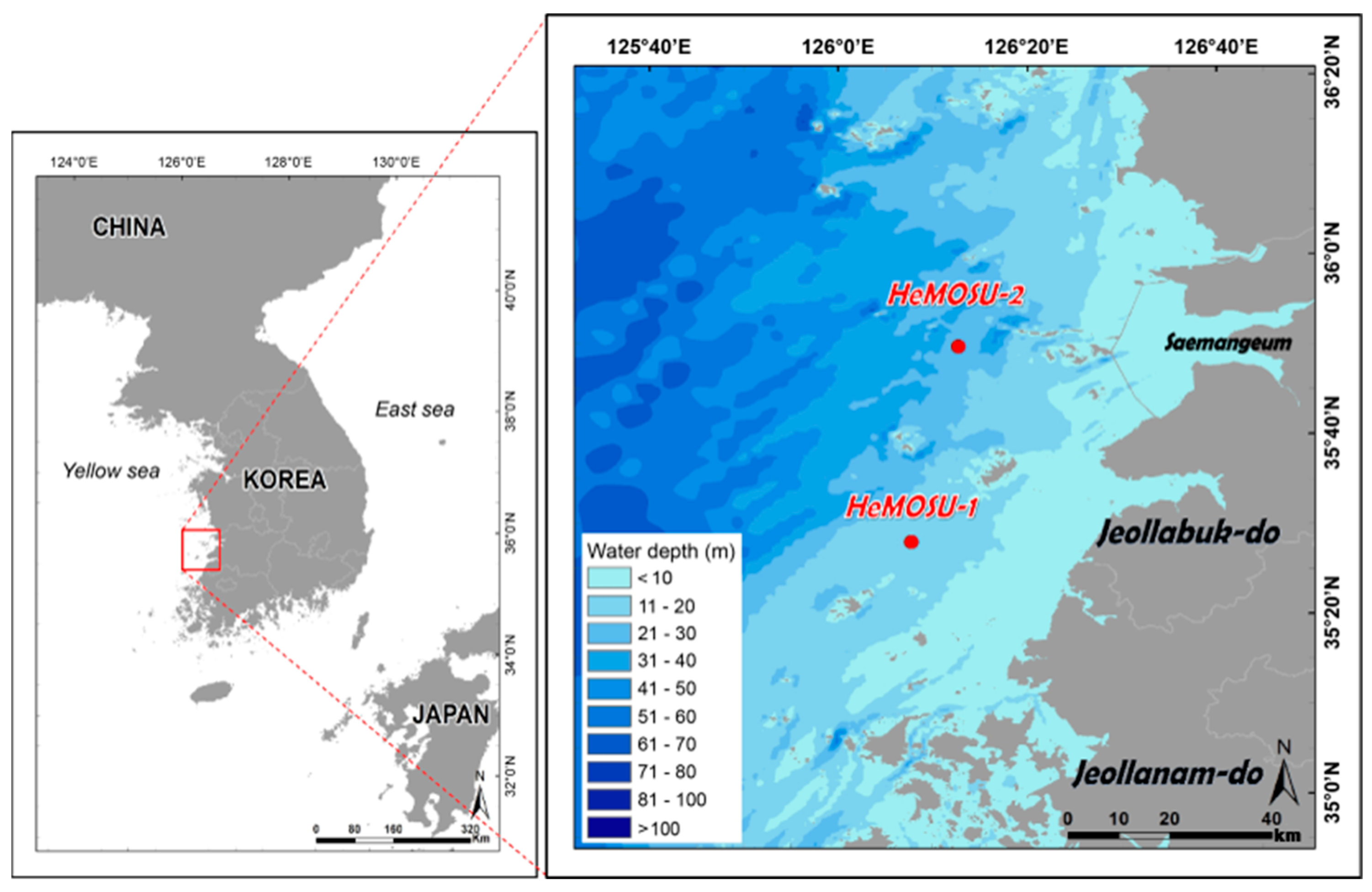
2. Observation Information and Water Surface Elevation Data

The Korea Electric Power Corporation has established two oceanographic and meteorological observation towers on the western coast aimed at facilitating the development of an offshore wind farm and investigating prevailing wind and sea conditions. Additionally, the HeMOSU (Herald of Meteorological and Oceanographic Special Research Units), which marked the beginning of marine meteorological research structures, was positioned in the waters near Wido-myeon, Buan, and Okdo-myeon, Gunsan, during 2010 and 2013, respectively. These structures actively gather and assess real-time wind condition data (including wind speed, wind direction, 3D wind speed, temperature, humidity, atmospheric pressure, and rainfall) as well as sea condition data (such as waves, flow velocity, and tide) [21]. Concerning their operational approach, these units operate through a combination of code-division multiple access communication and satellite channels, ensuring an ongoing accumulation of data for utilization in site design, maintenance, and environmental impact analysis. Descriptions and locations of the meteorological observation towers are provided in

Table 1. Information from the HeMOSU-1 and 2 meteorological observation towers.

	Platform Name
	HeMOSU-1	HeMOSU-2
Classification	Maximum height: 100 m Water depth: 13.5 m Foundation type: Jacket (weight: 200 tons)	Maximum height: 120 m Water depth: 30 m Foundation type: Suction Tripod (weight: 370 tons)
Characteristic	First offshore meteorological tower in the Republic of Korea First establishment of integrated measurement system in the Republic of Korea	Offshore structure where suction piles were first applied in the Republic of Korea First design approval meteorological tower in the Republic of Korea
Longitude and latitude	126°07′45″ E, 35°27′55″ N	126°12′45″ E, 35°49′40″ N

and Figure 2.

The Waveguide system, developed by Radac B.V. in 1996, facilitates wave height and direction observation. This system is incorporated into the meteorological observation tower platform and is under the control of a Waveguide server. Data transmission is achieved through a remote system (as detailed in

Table 2. Waveguide server details.

Model		Waveguide Radar System
Manufacturer		RADAC (NL)
Sampling rate		5 Hz
Wave heights		0–60 m
Wave periods		1–100 s
Accuracy water level		1.0 cm
Electrical	Radar frequency	9.9–10.2 GHz
	Modulation	Triangular FM
	Power requirements	24–64 VDC, 6 W/radar
Mechanical	Dimensions	26/21 cm (diameter/height)
	Weight	Approximately 9 kg
Environmental conditions	Temperature	−40 °C to 65 °C
	Humidity	0–100%
Accuracy	Water surface elevation	$\pm 1.0 \mathrm{cm}$
	Wave height	$\pm 3.0 \mathrm{cm}$
	Wave period	$\pm 50 \mathrm{ms}$

). Employing the Standard Wave Analysis Package (SWAP) method; the Waveguide system conducts computations utilizing observed water surface elevation data to derive diverse wave parameters. These encompass wave time-domain processing data ($H_i,T_i$), wave spectral domain processing data ($H_{m_0},T_p,m_0,\dots$), and wave spectrum data (Czz10, …) [22]. For the wave spectral domain processing data and wave spectrum data in their raw state, a 10% cosine tapering correction is applied, with appropriate wind–wave periods falling within the 2–33 s range. Subsequently, wave parameters are computed using the spectrum analysis method in the frequency domain, employing FFT.

The time interval of the observation data ($\mathsf{\eta }\left(t_i\right)$) was 200 ms (0.2 s). The period of observation data employed in this study spanned from July 2013 to July 2014 (approximately 6 months, i.e., 170 days, excluding instances of omission) for HeMOSU-1. For HeMOSU-2, the period was from November 2013 to April 2014 (approximately 4 months, i.e., 133 days, excluding instances of omission). Data omissions could stem from system errors and maintenance intervals of the equipment.

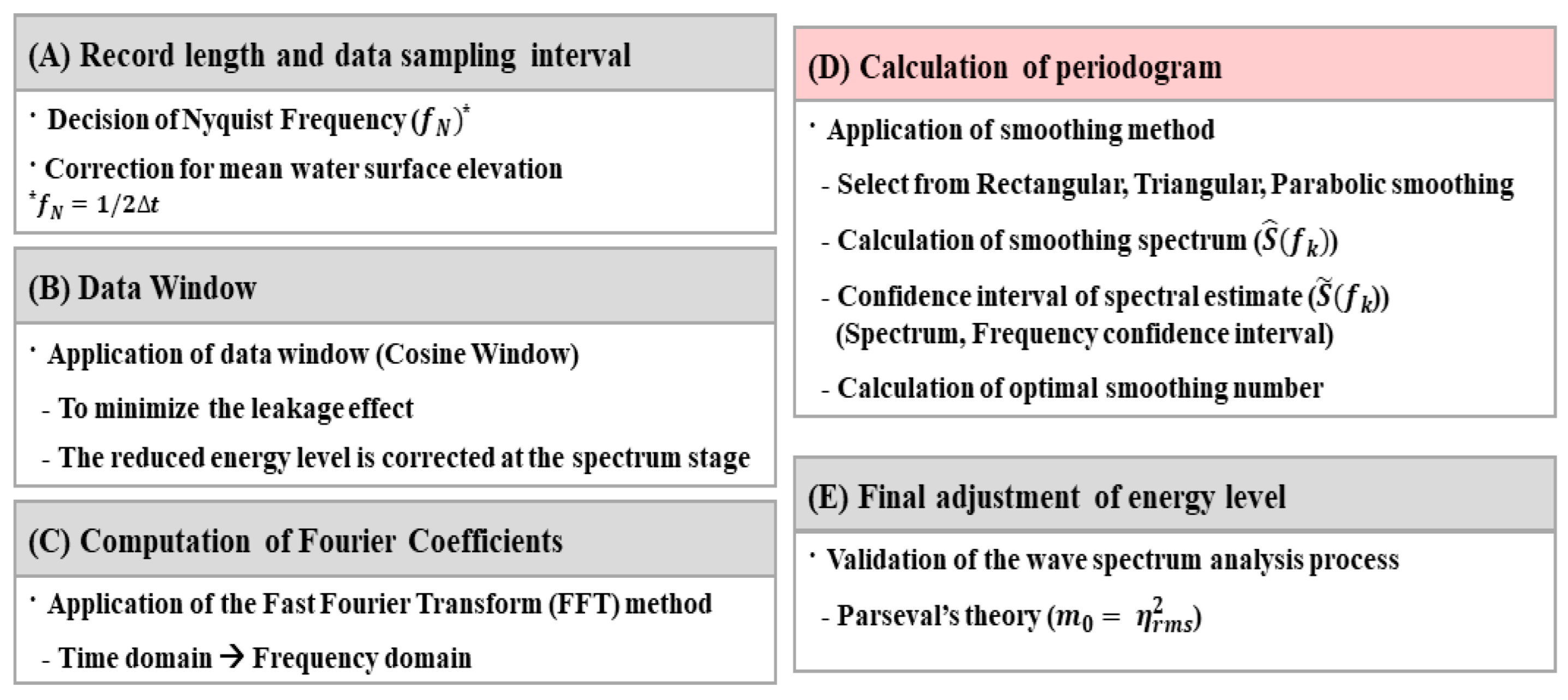
3. Method for Analysis

3.1. Methodology of Smoothing

Wave spectrum analysis encompasses both the time and frequency domains. In the time domain, the process involves (1) correcting the mean water level, (2) implementing a data window technique to mitigate energy leakage that occurs when analyzing actual time-series data where the domain is not an integer multiple ($n\mathsf{\Delta }f$) of the frequency interval ($\mathsf{\Delta }f$), and (3) applying a data filter method to exclude specific periods. In the frequency domain, the process entails converting from the time domain to the frequency domain using methods such as FFT and conducting a periodogram analysis. The periodogram method means that in spectrum estimation, the periodogram method carries out discrete Fourier transformation on water surface elevation data, and considers only the magnitude component of the transformed numerical value (because the values are the complex number) as a spectrum. While the analysis process in the time domain is notably standardized and straightforward, the analysis process in the frequency domain is more intricate, necessitating a more sophisticated approach. Typically, wave parameter calculations for deep water sites rely on the spectrum’s area estimated via frequency domain analysis and the frequency corresponding to the highest energy density. However, due to substantial confidence intervals associated with estimated spectrum values, uncertainty issues can arise in the estimated values, prompting the need for supplementary analysis.

FFT is commonly employed to analyze time-series data following observation data corrections in the frequency domain. However, to offer flexibility in selecting the amount of data for analysis, rather than confining it to $N=2^n$, this study employs the periodogram method. This method computes and converts Fourier coefficients to the frequency domain, as depicted in Equation (1).

$$\mathsf{\eta }\left(t_{*}\right)=\frac{A_0}{2}+{\displaystyle {{\displaystyle \sum }}_{k=1}^{\frac{N}{2}-1}}\left(A_k\cos \frac{2\pi k}{N}{t}_{*}+B_k\sin \frac{2\pi k}{N}{t}_{*}\right)+\frac{A_{N/2}}{2}\cos \pi t_{*}$$

(1)

where

$$t_{*}=\mathrm{t} / \mathsf{\Delta }\mathrm{t} : t_{*}=1,2,3,\dots , N$$

(2)

$$\begin{array}{cc}{A}_k=\frac{N}{2}{\displaystyle \sum }_{t_{*}=1}^N\eta \left(t_{*}\right)\cos \frac{2\pi k}{N}{t}_{*}& :0 \le k \le N/2\\ B_k=\frac{N}{2}{\displaystyle \sum }_{t_{*}=1}^N\eta \left(t_{*}\right)\sin \frac{2\pi k}{N}{t}_{*}& :1 \le k \le \frac{N}{2}-1\end{array}$$

(3)

To enhance the precision of spectrum estimation, the data smoothing method employing the bias-variance trade-off theory was employed, as demonstrated in the subsequent equation. The bias-variance trade-off constitutes a pivotal theory aimed at minimizing errors such as overfitting or underfitting when generalizing a random distribution. This concept can be expressed as Equation (4).

$$\mathrm{E}{[\left(\widehat{X}-X\right)]}^2={\left(X-E(\widehat{X})\right)}^2+(\mathrm{E}\left(\widehat{X}\right)-{[E\left(\widehat{X}\right)]}^2)$$

(4)

where $X$ is the real spectrum value and $\widehat{X}$ is the estimated spectrum value. Furthermore, in Equation (4), the left side corresponds to the mean square error (MSE), $\mathrm{E}(\widehat{X})-{[E(\widehat{X})]}^2$ is the variance, and $X-E\left(\widehat{X}\right)$ is the bias.

The smoothing technique employed within this study involved the estimation of spectral density ($I_k$) followed by the computation of the smoothing function ${\psi }_j$, as demonstrated in Equations (5) and (6).

$$I_k=\left[\begin{array}{cc}N\left(A_k^2+B_k^2\right)& :1 \le k \le \frac{N}{2}-1\\ N{A}_0^2& :k=0\\ N{A}_{N/2}^2& :k=N/2\end{array}\right]$$

(5)

$$\mathrm{S}\left(f_k\right)=I_k·C_p·\left(\Delta t/2\right)$$

(6)

where $C_p$ denotes the correction factor accounting for the reduction in the estimated spectral energy density. The smoothing procedure for the spectrum, computed through the abovementioned equations, can be ascertained using Equations (7)–(9).

$$\widehat{S}\left(f_k\right)={\displaystyle {{\displaystyle \sum }}_{j=-n}^n}{\psi }_{j}S\left(f_{k+j}\right)$$

(7)

$${\displaystyle {{\displaystyle \sum }}_{j=-n}^n}{\psi }_j=1$$

(8)

$${\psi }_j=\left\{\begin{array}{ccc}{\psi }_1\left(f_j\right)=& \frac{1}{n}& :-\left[\frac{n-1}{2}\right]\le j\le \left[n/2\right]\\ {\psi }_2\left(f_j\right)=& \frac{1}{\overline{{\psi }_2}}\left\{1-\frac{\left|j\right|}{\left[\left(n-1\right)/2\right]}\right\}& :-\left[\frac{n-1}{2}\right]\le j\le \left[n/2\right]\\ {\psi }_3\left(f_j\right)=& \frac{1}{\overline{{\psi }_3}}\left\{1-{(\frac{\left|j\right|}{\left[\left(n-1\right)/2\right]})}^2\right\}& :-\left[\frac{n-1}{2}\right]\le j\le \left[n/2\right]\end{array}\right\}$$

(9)

where $n$ is the smoothing parameter and ${\psi }_j$ is the smoothing function. In the above equation, ${\psi }_1$ is rectangular smoothing, ${\psi }_2$ is triangular smoothing, and ${\psi }_3$ represents parabolic smoothing. In this study, triangular smoothing (${\psi }_2$) was chosen due to computational efficiency and time considerations; it involves overlapping half of the data for analysis.

3.2. Result Validation Method Using Parseval’s Theory

However, owing to the processing methods employed in complex analyses, the energy level might exhibit slight deviations from the input value, underscoring the need for a validation step [4]. To validate the spectrum analysis method, this study employed Parseval’s theorem, which asserts that the total energy in the time domain equals the variance of waveforms in the frequency domain [23]. This theorem can be formulated as follows:

$${\displaystyle {{\displaystyle \sum }}_{i=1}^N}{\eta }^2\left(t_i\right)=\frac{2}{N}{\displaystyle {{\displaystyle \sum }}_{k=1}^{\raisebox{1ex}{$N$}\!\left/ \!\raisebox{-1ex}{$2$}\right.}}S\left(f_k\right)$$

(10)

In the context of applying a spectrum, the number of data points ($N$) is constrained to values ranging from 1, 2, 3, …, to N/2. Once this is established, the Nyquist frequency essential for interpreting the spectrum can be represented as $f_N=\raisebox{1ex}{$1$}\!\left/ \!\raisebox{-1ex}{$\left(2\mathsf{\Delta }t\right)$}\right.$ (with a minimum period of $2\mathsf{\Delta }t$), and the calculation is executed utilizing the corresponding ratio. Furthermore, the zero moment of the estimated wave spectrum ($m_0$), indicating the area of the spectrum, along with the total energy of the observed data (${\eta }_{rms}^2$), is expressed in Equations (11) and (12).

$$m_0= \mathsf{\Delta }f {\displaystyle {{\displaystyle \sum }}_{k=1}^{\raisebox{1ex}{$N$}\!\left/ \!\raisebox{-1ex}{$2$}\right.}}\frac{S\left(f_k\right)}{f_N}=\frac{2}{N} {\displaystyle {{\displaystyle \sum }}_{k=1}^{\raisebox{1ex}{$N$}\!\left/ \!\raisebox{-1ex}{$2$}\right.}}S\left(f_k\right)={\eta }_{rms}^2$$

(11)

$${\eta }_{rms}=\sqrt{\frac{{\displaystyle {{\displaystyle \sum }}_{i=1}^N}{\eta }^2\left(t_i\right)}{N}}$$

(12)

where $\mathsf{\Delta }f$ is the frequency interval, which can be expressed as $\mathsf{\Delta }f=1/\left(N\mathsf{\Delta }\mathrm{t}\right)$.

Since the peak period is one of the main parameters used in the wave spectrum distribution model, numerical wave model (SWAN), design wave calculation, and extreme value analysis, it is important to accurately estimate it. However, when peak wave period utilization is limited by the irregular spectral shape, which mainly occurs at low wave heights, the mean period may be used. The mean period ($\overline{ T}$) of the wave defined by the wave train analysis can be calculated as the mean period ($T_{02}$) using the second moment ($m_2$) of the spectrum (Equations (13) and (14)).

$$\overline{T}\approx T_{02}=\sqrt{m_0/m_2}$$

(13)

$$m_2={{\displaystyle \int }}_0^{\infty }{f}^{2}S\left(f\right)df$$

(14)

When calculating the average period from the spectrum, Equation (13) is typically used. However, there has been a recent increase in cases, mainly in Europe, where the average period calculated from Equations (15) and (16) has been used.

$$T_{m-1,0}=m_{-1}/m_0$$

(15)

$$m_{-1}={{\displaystyle \int }}_0^{\infty }{f}^{-1}S\left(f\right)df$$

(16)

Using Equations (13) and (15), the mean period ($T_{02}$, $T_{m-1,0}$) of the HeMOSU sea area was calculated, and the distribution of peak and mean wave period were confirmed.

The calculation range of the zero moment ($m_0$) and second moment ($m_2$), which are essential for calculating the wave period, was not calculated for the entire spectrum but rather analyzed considering $0.5f_p\le f_p\le 6.0f_p$, the frequency range empirically suggested by Goda (2010) [4].

4. Results and Discussion

4.1. Validation of Wave Parameter Result

In this study, a wave spectrum analysis was conducted utilizing water surface elevation data collected via the Waveguide systems installed in HeMOSU-1 and HeMOSU-2. Furthermore, two complementary methods were employed to enhance result accuracy. It is imperative to validate the acquired wave data through this analytical approach. Therefore, an examination was conducted to evaluate the correlation analysis and peak period ratio for the peak wave period ($T_p$), calculated using the wave spectrum method used in this study, and the peak wave period ($T_p$), calculated using the Waveguide (as illustrated in Figure 3). Moreover, supplementary validations were executed by applying Parseval’s theorem, represented as Equation (10).

To scrutinize the pattern alteration and appropriateness of the derived wave parameters, the correlation between the wave parameters calculated via wave spectrum analysis using the Waveguide system and those obtained through the wave spectrum analysis method proposed in this study was assessed employing the Pearson, Kendall, and Spearman methods [24].

Looking at the ratio of the determined peak wave period, in the case of HeMOSU-1, the average of $T_{p,\mathrm{ThisStudy}}$ was 5.417 s, and outliers (values exceeding the maximum value) were 5.7% of the total data. The average of $T_{p,\mathrm{SWAP}}$ was 4.977 s, the outlier was 4.51% of the total data, and the average of $T_p$ calculated by the two methods showed a difference of about 8.12%. Meanwhile, in the case of HeMOSU-2, the average of $T_{p,\mathrm{ThisStudy}}$ was 5.803 s, and outliers (values exceeding the maximum value) were 0.67% of the total data. The average of $T_{p,\mathrm{SWAP}}$ was 5.349 s, the outlier was 0.05% of the total data, and the average of $T_p$ calculated by the two methods showed a difference of about 7.82%.

It is believed that the difference in $T_p$ estimated at each point occurs because of the difference in analysis method from SWAP. However, when calculating the IQR (Interquartile Range), which means the degree of distribution of data based on the median for each $T_p$, it can be seen that the IQR of the $T_p$ for each point appears similar.

The three-type (Pearson, Kendall, and Spearman) correlation analysis for $T_p$ yielded correlation coefficient (CC) values of more than 0.8, respectively (as illustrated in Figure 4). Discrepancies between the two methods could stem from the smoothing techniques employed in this study. A comprehensive elaboration on the impacts of these analysis methods is provided in Section 4.2.

To corroborate the findings of the wave spectrum analysis conducted in this study, a theory stating that the variance ($m_0$) of the waveform equates to the total energy (${\eta }_{rms}^2$) of the observed data that were employed, as depicted in Equation (10) [4]. The correlation analysis outcomes for the two parameters in both HeMOSU-1 and HeMOSU-2 demonstrated CC values of 0.9994 and 0.9991, respectively. These results suggest statistical equivalence between the two parameters (as illustrated in Figure 5).

4.2. Smoothing Effect

The wave spectrum has significant changes in wave height and period estimation depending on frequency and shape, and the confidence interval (CI) range of the spectrum estimated under the fundamental resolution conditions ($\Delta f=1/(N\Delta t$)) is notably extensive. Statistically, a very large confidence interval means that the range of the confidence interval is wide. The wider the range of the confidence interval, the higher the probability of including the parameter, but this means that the information about the value of the parameter is very weak. In general, during confidence interval estimation, a 95% confidence interval is often constructed using the chi-square distribution, as illustrated in Equation (17). This analysis was conducted with consideration for phenomena adhering to a chi-square distribution [4,25].

$$\tilde{S}\left(f_k\right)=S\left(f_k\right)\frac{{\chi }_{2n}^2}{2n}$$

(17)

In the process of estimating the peak frequency (the frequency at which the spectrum value is at maximum), if the confidence interval problem is taken into consideration, problems may arise in estimating the appropriate peak frequency. In cases where it is difficult to estimate the peak frequency at once, such as a bimodal spectrum, the value of the largest spectrum must be selected at a level that shows a significant difference from the second largest spectrum value to estimate the peak frequency, which is one of the most important estimation information in spectrum analysis. Ultimately, a process of reducing the range of the confidence interval is necessary, and for this purpose, it is common to apply a smoothing method. Through this process, it is possible to estimate the maximum spectrum information showing a significant difference, and at this time, the maximum frequency can be estimated. In Figure 6, the change in confidence interval when smoothing is applied to the wave spectrum of $H_s=4.07 \mathrm{m}, \mathrm{and} T_p=12.59 \mathrm{s}$ is presented.

Through the calculation of the confidence interval for the estimated spectrum, the confidence interval range for the peak part of the estimated spectral density was 49.38~229.12 ${\mathrm{m}}^2\mathrm{s}$ (blue box part in Figure 6), while the confidence interval range for the spectral density calculated through smoothing was 13.27~61.59 ${\mathrm{m}}^2\mathrm{s}$ (red box part in Figure 6). Consequently, the confidence interval range was reduced by approximately 27% after applying the smoothing technique. In this way, it can be seen that when smoothing is applied, the range of the confidence interval is reduced by a large difference, and the accuracy of peak frequency estimation is improved. Moreover, an investigation was conducted into the alteration patterns of peak wave periods with respect to varying ranges of significant wave heights at HeMOSU-1 and HeMOSU-2, with the results presented in Figure 7 and Figure 8.

Regarding the estimated spectrum at 4.07 m, representing the maximum significant wave height ($H_s$) at HeMOSU-1, the peak wave period ($T_p$) remained constant at 11.87 s before and after smoothing, signifying no significant alteration. In contrast, for $H_s=3.01 \mathrm{m}$, $T_p$ decreased from 13.38 to 11.78 s, while for $H_s=2.00 \mathrm{m}$, $T_p$ decreased from 11.14 to 10.54 s, and for $H_s=1.00 \mathrm{m}$, $T_p$ increased from 7.2 to 8.31 s, demonstrating a distinct change pattern. Similarly, at 5.14 m, corresponding to the maximum significant wave height ($H_s$) at HeMOSU-2, the peak period ($T_p$) was 11.61 s for both the estimated spectrum and the spectrum after smoothing. For $H_s=4.02 \mathrm{m}$, $T_p$ remained at 12.59 s, indicating no alteration in the high frequency region, as observed in HeMOSU-1. However, for $H_s=3.01 \mathrm{m}$, $T_p$ decreased from 12.23 to 10.68 s, while for $H_s=2.00 \mathrm{m}$, $T_p$ decreased from 11.29 to 10.30 s. Lastly, for $H_s=1.04 \mathrm{m}$, $T_p$ decreased from 6.56 to 4.20 s, exhibiting a discernible change in pattern. Because the area of the spectrum represents the zeroth moment ($m_0$) applied to calculate the significant wave height, the peak spectral density of the spectrum was found to decrease as the significant wave height became smaller. In addition, when the significant wave height is small, the spectrum shape is not concentrated due to effects such as swell, and a bimodal spectrum shape is mainly observed, which causes problems in estimating the peak period. However, in the case of a spectrum to which smoothing is applied, the confidence interval is greatly reduced compared to the existing spectrum, so the uncertainty problem in peak period estimation can be resolved, and it is judged appropriate to use the peak period calculated through this.

The alteration in the peak wave period is presumed to arise in the form of an unstable spectral distribution, characterized by occurrences of multiple peaks and the dispersal of wave spectral energy density as significant wave height decreases. Conversely, when smoothing is performed on the estimated spectrum, as the smoothing number increases, the spectrum shifts toward the low frequency domain. This is judged to be the numerical effect of data loss on the applied smoothing number. This transition is attributed to a numerical effect due to data loss relative to the number of applied smoothing iterations. Addressing this concern hinges on judiciously determining the smoothing parameter ($n$) outlined in Equation (9). For this determination, the root mean square error (RMSE) is computed using Equation (18) while varying n. Subsequently, the n value yielding the minimum error is selected.

$${\mathrm{RMSE}}_{min}=\sqrt{\frac{{\sum }_{k=1}^n{[\widehat{S}\left(f_k\right)-S^{*}\left(f_k\right)]}^2}{N_s}}$$

(18)

where $S^{*}\left(f_k\right)$ represents the reference smoothing spectrum adopted for the RMSE calculation. This involves kernel regression smoothing with a Local Plug-In technique applied using the ‘lokerns’ function within the ‘lokerns’ package of the R program. $N_s$ denotes the number of spectrum data points [26].

The rationale for utilizing the Local Plug-In (LPI) method stems from the wave spectrum’s heteroscedastic shape, marked by variations in dispersion across different sections. The Direct Plug-In (DPI) method, which is straightforward for smoothing analyses, is not employed due to its unaddressed bandwidth estimation issue. DPI smoothing entails applying a singular bandwidth to all sections marked for smoothing. In general, in kernel regression estimation, underestimation may occur with small bandwidths, while overestimation can arise with large bandwidths [4]. Given these considerations, the kernel regression approach inherent in the LPI method, offering precise smoothing, was selected [26]. To compute the optimal smoothing parameter, Figure 9 illustrates the variation in RMSE as the smoothing parameter changes, alongside the alteration in the confidence interval for a significant wave height of 4.00 m at HeMOSU-1 and 5.12 m at HeMOSU-2.

Upon analyzing changes in the confidence interval for the most prominently expressed significant wave heights at HeMOSU-1 and HeMOSU-2, it was established that the optimal number of smoothing, as determined by the smallest RMSE, was nine for HeMOSU-1 and seven for HeMOSU-2. In HeMOSU-1, this yielded a change in the confidence interval range of the spectrum ($\mathsf{\Delta }{S}_{CI}$) from 0.98~142.69 ${\mathrm{m}}^2\mathrm{s}$ to 11.90~45.58 ${\mathrm{m}}^2\mathrm{s}$ compared to no smoothing. Additionally, the variation in frequency resolution range ($\mathsf{\Delta }{f}_{RE}$) spanned from 0.091~0.092 Hz to 0.07~0.08 Hz. Similarly, for HeMOSU-2, the optimal smoothing parameter was seven, resulting in a change in the spectrum’s confidence interval range from 0.811~117.36 ${\mathrm{m}}^2\mathrm{s}$ to 15.90~73.79 ${\mathrm{m}}^2\mathrm{s}$, and a modification in frequency resolution range from 0.0996~0.101 Hz to 0.088~0.097 Hz.

As the amount of data used for smoothing increases, the smoothing becomes very smooth. In other words, as the smoothing number increases, the range of the confidence interval for the wave spectral density corresponding to the y-axis tends to continuously decrease. However, according to the Bias-Various Trade-off theory, the confidence interval of the frequency resolution corresponding to the x-axis increases infinitely, so the appropriate number of smoothing must be calculated. Consequently, a suitable number of smoothing iterations must be meticulously calculated. The outcomes of this calculated optimal smoothing process are showcased in Figure 10.

Upon calculating the optimal smoothing parameters for various wave height sections, it was determined that for significant wave heights $H_s>4$, the suitable smoothing numbers for HeMOSU-1 and HeMOSU-2 were seven and nine, respectively. When the range was $3<H_s<4$, the optimal smoothing number was 11 for both locations. For the range of $2<H_s<3$, it was 11 for HeMOSU-1 and 15 for HeMOSU-2. In the segment of significant wave heights between $1<H_s<2$, the appropriate smoothing number was 15 for both locations. Conversely, for wave height ranges less than 1 ($H_s<1$), the optimal smoothing numbers were 25 for HeMOSU-1 and 19 for HeMOSU-2. Evidently, the smoothing number exhibited an ascending trend at both sites as significant wave height decreased. This trend suggests that challenges encountered when applying smoothing are due to the unstable distribution of the wave spectrum.

4.3. Estimation of Representative Wave Period

For many coastal sites, mean wave periods such as T₀₂ or T_m−1,0 may be required in coastal engineering calculations [19,20], especially where multiple energy peaks occur with (relatively) low wave heights.

Looking at the distribution trend of the representative period ($T_{02},T_{m-1,0}$) of HeMOSU-1, as shown in Figure 11a–c, the mean of each representative period was $T_p=$6.01 s, $T_{02}=$3.48 s, and $T_{m-1,0}=$4.11 s, respectively. The peak wave period was approximately 1.73 times greater than the average period ($T_{02}$) and approximately 1.46 times greater than the mean period ($T_{m-1,0}$). Additionally, each mean period, $T_{m-1,0}$ was approximately 1.18 times greater than $T_{02}$. In the case of HeMOSU-2, as shown in Figure 11d–f, the mean of the representative period was $T_p=$6.53 s, $T_{02}=$3.90 s, and $T_{m-1,0}=$4.56 s, respectively, showing the same trend as HeMOSU-1. The peak wave period was approximately 1.67 times greater than the mean period ($T_{02}$) and approximately 1.43 times greater than the mean period ($T_{m-1,0}$). Additionally, for each mean period, $T_{m-1,0}$ was approximately 1.17 times greater than $T_{02}$.

In the case of peak wave periods at two points, most periods tended to be distributed between approximately 4.5 and 7.5 s. Additionally, the mean period ($T_{02}$) was distributed from approximately 2.5 to 4.5 s, and the mean period ($T_{m-1,0}$) was distributed from approximately 3.0 to 5.5 s. These results confirm that the wave period distribution of the target sea area appears similar to that demonstrated by Lee et al. (2021) [27].

Additionally, the relationship between peak wave period ($T_p$) and mean wave period ($T_{m-1,0})$ calculated in this study was estimated. The correlation equation between representative wave periods can be calculated through correlation analysis, and the superiority of the estimated linear model can be judged using the coefficient of determination [28]. In this way, the relationship between representative wave height and representative period can be defined as a linear relationship, such as $y=ax+b$, and the analysis results are presented in Figure 12, below. In the case of HeMOSU-1, the relationship between the peak period and the average period was $T_p=1.153T_{m-1,0}+0.852$, the coefficient of determination ($R^2$) was 0.782, and the correlation coefficient was 0.831. HeMOSU-2 showed a relationship of $T_p=1.325T_{m-1,0}+0.526$, the coefficient of determination ($R^2$) was calculated to be 0.837, and the correlation coefficient value was calculated to be 0.864. Goda (2010) [4] proposed $T_p=\left(0.99~1.54\right)\overline{T}$ as the relationship between the mean wave period ($\overline{T}$) and peak period ($T_p$) calculated through wave train analysis. When comparing this relation with the linear relation calculated in this study, it can be seen that the coefficient value of the calculated relation is similar to the previously proposed relation (as shown in Figure 12).

5. Conclusions

In this study, employing water surface elevation data collected from HeMOSU-1 and HeMOSU-2 installations on the western coast of the Republic of Korea, the issue of peak period calculation during wave spectrum analysis was addressed, and resolution methodology was suggested. The primary outcomes derived from this investigation are summarized as follows.

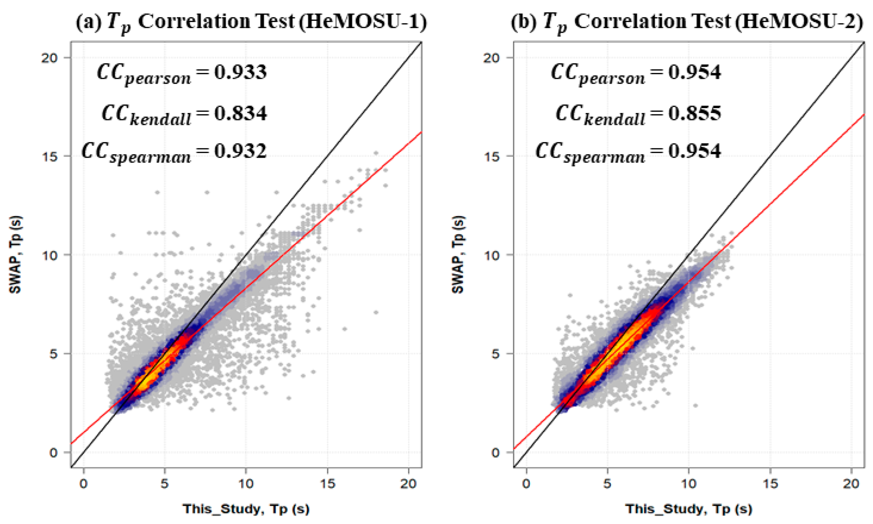
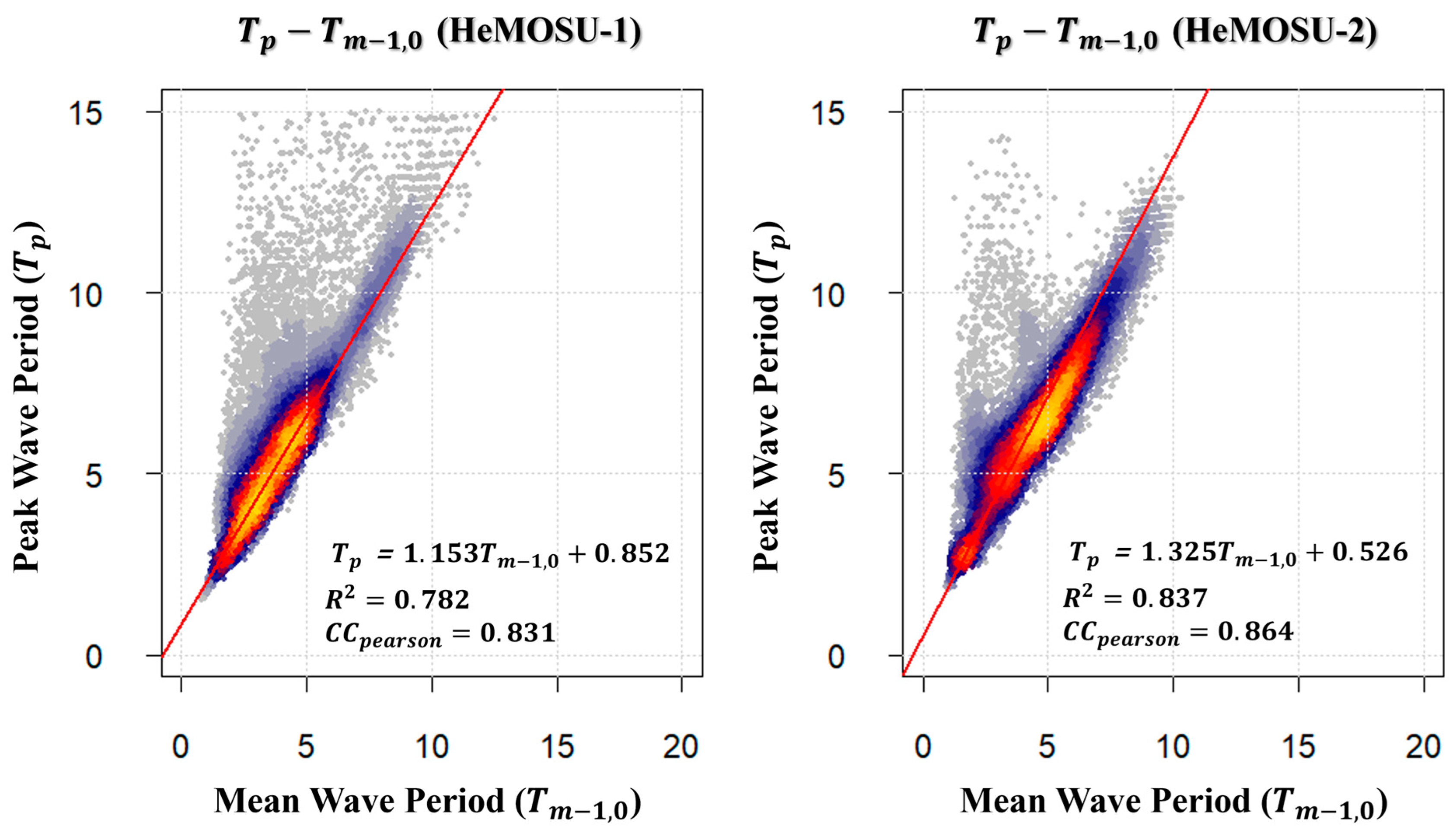
• To ascertain the variation pattern and suitability of the calculated peak wave period, a correlation analysis was conducted on the peak wave period derived from observation equipment and the peak period analyzed with the applied smoothing technique in this study. The computed CC (Pearson, Kendall, Spearman method) for HeMOSU-1 and HeMOSU-2 locations was more than 0.8, respectively. While the majority of peak wave periods clustered around 3–5 s, any variations in peak wave periods observed in other intervals were attributed to the impact of the applied smoothing method.
• In typical wave parameter estimation via wave spectrum analysis, verification of the analysis approach is commonly executed using Parseval’s theory, which equates the variance of waveforms to the total energy of observed data. Correlation analysis employing the two calculated variables (${\eta }_{rms}^2, m_0$) yielded highly robust CC of 0.9994 and 0.9991, demonstrating their statistical equivalence. This confirms the integrity of the wave spectrum analysis undertaken in this study.
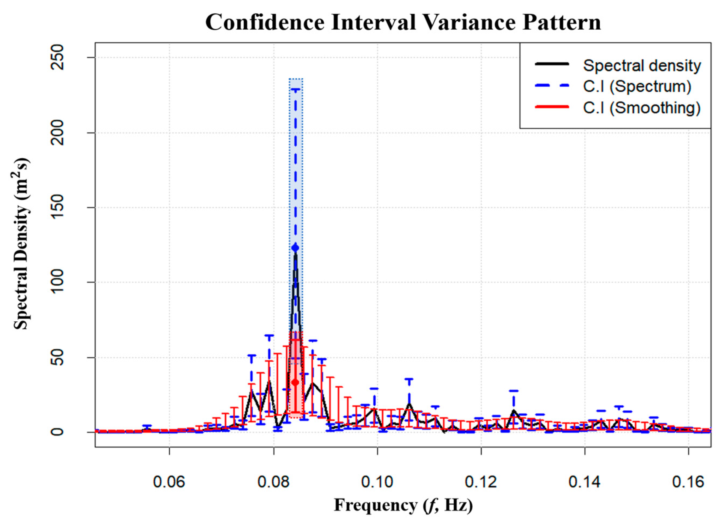
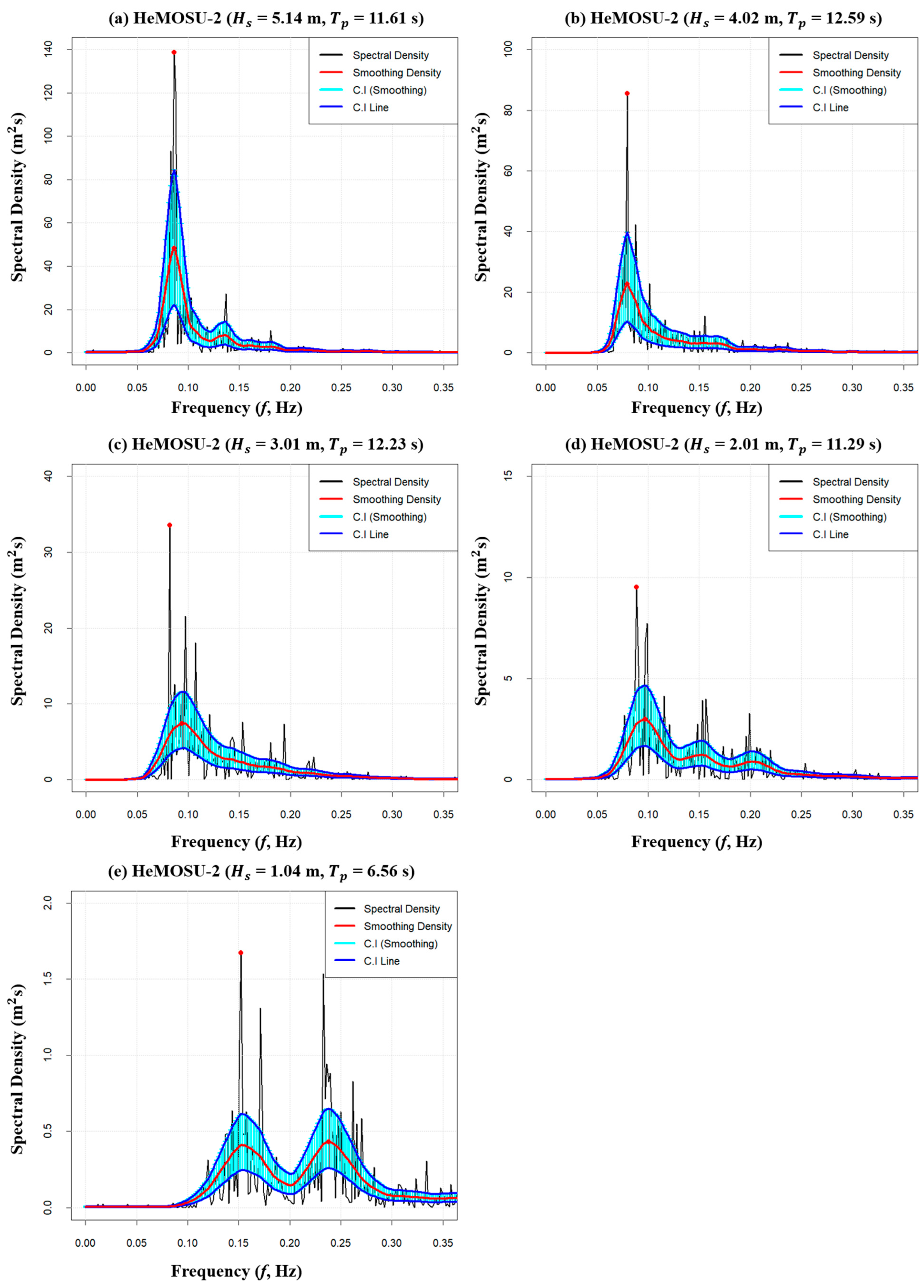
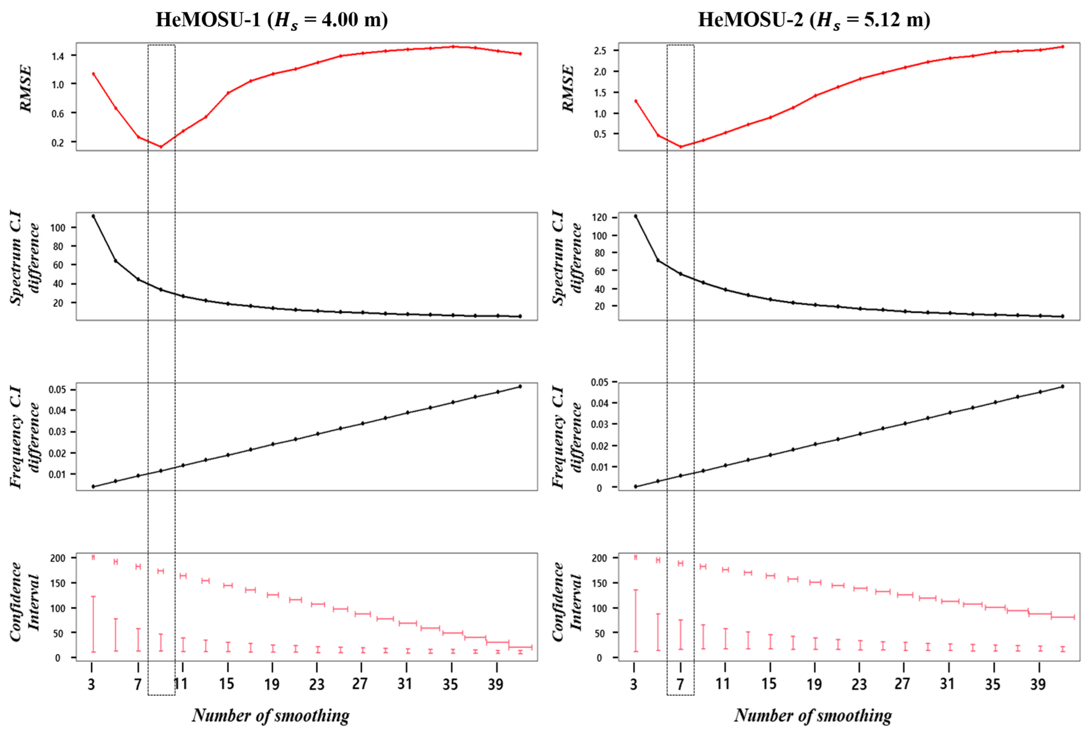
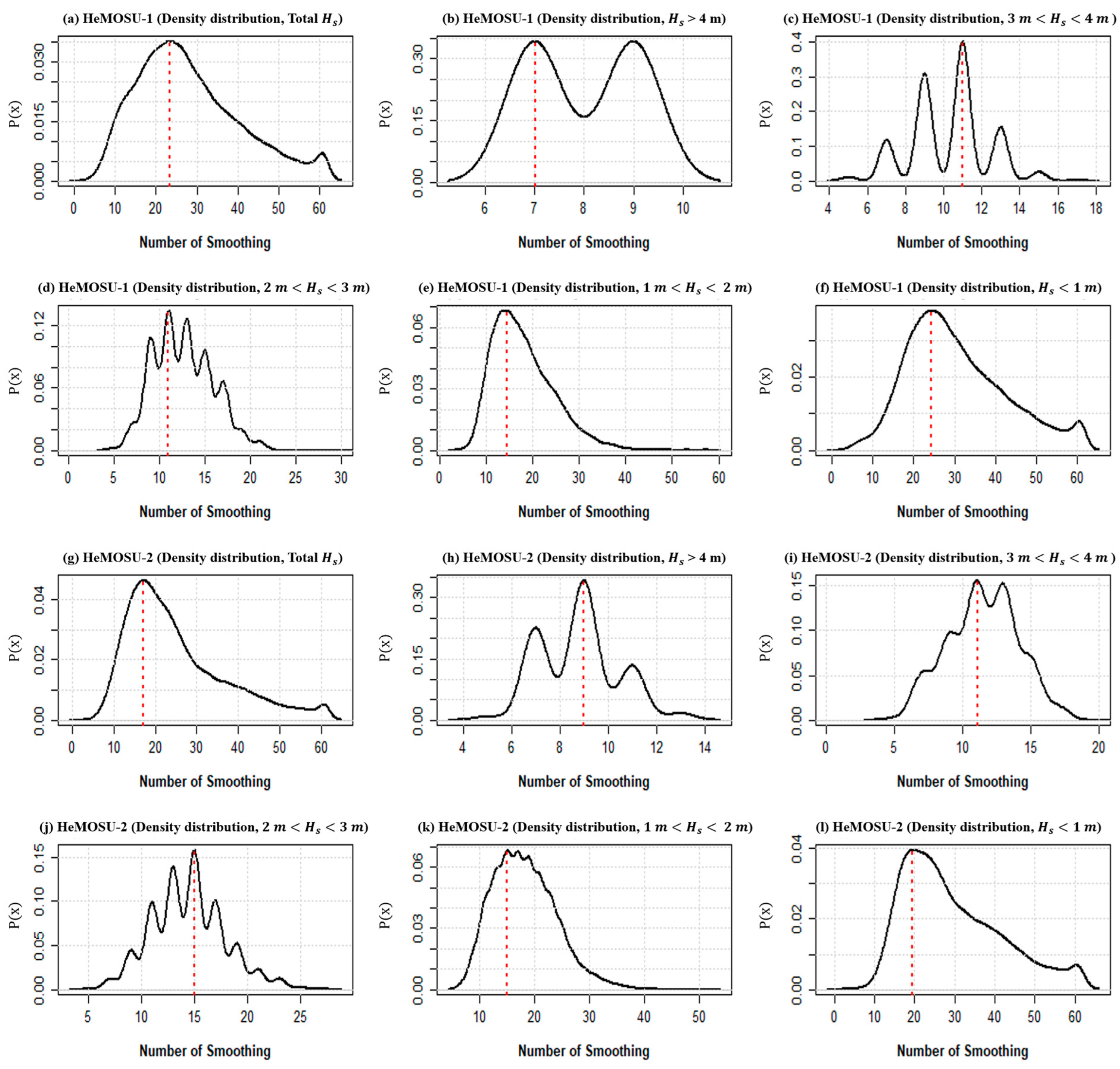
• The estimated energy density of wave spectra exhibits notably broad confidence intervals. To address the uncertainty challenges within the confidence interval during peak wave period estimation via wave spectrum analysis, smoothing was implemented employing various statistical techniques. Through estimation involving the 95% chi-square distribution, post-smoothing confidence intervals exhibited an average reduction of about 27%. Additionally, investigating peak wave period variation fluctuations concerning the range of significant wave heights revealed minimal variation in the high significant wave height range, characterized by concentrated spectral energy density. In contrast, a variation of approximately 1–2 s in peak wave period was evident, especially in lower significant wave height ranges. This phenomenon is attributed to complexities such as bimodal spectrum shape, where the spectral energy density exhibits an unstable pattern with diminishing significant wave height. Moreover, a refined smoothing number was calculated to enhance precision in smoothing relative to the significant wave height range. In other words, the analysis results show a negative correlation between the number of smoothed waves and the significant wave height: $C{C}_{HeMOSU-1}$: −0.66, $C{C}_{HeMOSU-2}$: −0.71 (the number of smoothed waves decreases as the significant wave height increases). This means that there are limits to applying the smoothing technique due to the unstable characteristic of the spectral energy density as the significant wave height decreases.

In general, the peak wave period is used in wave spectrum models such as PM, BM, and JONSWAP that classify ocean characteristics. However, when the spectrum shows a bimodal form, as the wave height becomes smaller, it may be difficult to select the peak period using smoothing, so the use of the mean wave period ($T_{02},T_{m-1,0}$) is increasing. The analysis of the distribution of the mean and peak wave periods in the target sea area revealed that the peak wave period was mostly distributed between approximately 4.5 and 7.5 s. Moreover, the mean period ($T_{02}$) was distributed between 2.5 and 4.5 s, and the mean period ($T_{m-1,0}$) was distributed between 3.0 and 5.5 s. Furthermore, the mean period ($T_{02},T_{m-1,0}$) was calculated to be 1.18 and 1.17 times greater than $T_{02}$, and the peak period and average period showed a difference of about 31.6% and 30.2% at each station. When using the mean period instead of the peak wave period, $T_{m-1,0}$ is often used rather than $T_{02}$. In this case, the mean period is judged to be sufficiently corrected in consideration of the peak wave period trend before use. The relationship between the peak wave period ($T_p$) and the mean wave period ($T_{m-1,0}$) calculated through spectrum analysis is the relationship between the mean wave period ($\overline{T}$) and the peak wave period ($T_p$) calculated through wave train analysis ($T_p=\left(0.99~1.54\right)\overline{T}$). Other than that, it has not been defined precisely. The relationships were calculated using the results calculated in this study, and as a result, the peak wave period ($T_p$)–mean wave period ($T_{m-1,0}$) relationships for HeMOSU-1 and 2 were calculated as $T_p=1.153T_{m-1,0}+0.852$ and $T_p=1.325T_{m-1,0}+0.526$.

In the realm of ocean data provision, diverse observation equipment is utilized to furnish information such as significant wave height, peak period, and wave direction. Since each observation device entails a distinct wave parameter estimation process, it becomes imperative to supply fundamental raw data, such as water surface elevation data. This study, constrained by the challenge of securing high-resolution raw data, such as water surface elevation data, focused its analysis on specific points.

References

1. Cho, H.-Y.; Kweon, H.-M.; Jeong, W.-M. A study on the optimal equation of the continuous wave spectrum. Int. J. Nav. Arch. 2015, 7, 1056–1063. [Google Scholar] [CrossRef]
2. Horikawa, K. Coastal Engineering, an Introduction to Ocean Engineering; University of Tokyo Press: Tokyo, Japan, 1978. [Google Scholar]
3. Mizuguchi, M. Individual wave analysis of irregular wave deformation in the nearshore zone. In Coastal Engineering 1982; American Society of Civil Engineers: Reston, VA, USA, 1982; pp. 485–504. [Google Scholar]
4. Goda, Y. Random Seas and Design of Maritime Structures; World Scientific Publishing Company: Singapore, 2010; Volume 33. [Google Scholar]
5. Stansell, P.; Wolfram, J.; Linfoot, B. Effect of sampling rate on wave height statistics. Ocean Eng. 2002, 29, 1023–1047. [Google Scholar] [CrossRef]
6. Mazeika, L.; Draudviliene, L. Analysis of the zero-crossing technique in relation to measurements of phase velocities of the Lamb waves. Ultragarsas/Ultrasound 2010, 65, 7–12. [Google Scholar]
7. Nishi, R.; Sato, M.; Kraus, N.C. Development of Wave Train Analysis Package: WAVETRAP; The Research Report of the Faculty of Engineering, Kagoshima University; Kagoshima University: Kagoshima, Japan, 1997; Volume 39, pp. 179–198. [Google Scholar]
8. Choi, H.; Jeong, S.T.; Cho, H.Y.; Ko, D.H.; Kang, K.S. Development of wave by wave analysis program using MATLAB. J. Korean Soc. Coast. Ocean Eng. 2017, 29, 239–246. (In Korean) [Google Scholar] [CrossRef]
9. Zheng, G.; Cong, P.; Pei, Y. On the improvements to the wave statistics of narrowbanded waves when applied to broadbanded waves. J. Geophys. Res. Atmos. 2006, 111. [Google Scholar] [CrossRef]
10. Thompson, E.F. Energy Spectra in Shallow US Coastal Waters. 1980. Available online: https://hdl.handle.net/11681/22206 (accessed on 15 September 2023).
11. Pierson, W.J.; Marks, W. The power spectrum analysis of ocean-wave records. Trans. Am. Geophys. Union 1952, 33, 834–844. [Google Scholar]
12. Casas Prat, M. Overview of Ocean Wave Statistics. 2008. Available online: https://upcommons.upc.edu/handle/2099.1/6034 (accessed on 15 September 2023).
13. Liu, P.C. Is the wind wave frequency spectrum outdated. Ocean Eng. 2000, 27, 577–588. [Google Scholar] [CrossRef]
14. Liu, P.C.; Babanin, A.V. Using wavelet spectrum analysis to resolve breaking events in the wind wave time series. In Annales Geophysicae; Copernicus GmbH: Göttingen, Germany, 2004; Volume 22, pp. 3335–3345. [Google Scholar]
15. Aranuvachapun, S. Parameters of Jonswap spectral model for surface gravity waves—II. Predictability from real data. Ocean Eng. 1987, 14, 101–115. [Google Scholar] [CrossRef]
16. Soares, C.G.; Carvalho, A.N. Probability distributions of wave heights and periods in combined sea-states measured off the Spanish coast. Ocean Eng. 2012, 52, 13–21. [Google Scholar] [CrossRef]
17. Rodriguez, G.R.; Soares, C.G. The bivariate distribution of wave height and periods in mixed sea states. J. Offshore Mech. Arct. Eng. 1999, 121, 102–108. [Google Scholar] [CrossRef]
18. IAHR Working Group on Wave Generation and Analysis. List of sea-state parameters. J. Waterw. Port Coast. Ocean Eng. 1989, 115, 793–808. [Google Scholar] [CrossRef]
19. Allsop, N.W.H.; Bruce, T.; De Rouck, J.; Kortenhaus, A.; Pullen, T.; Schüttrumpf, H.; Troch, P.; Zanuttigh, B. EurOtop II Manual on Wave Overtopping of Sea Defences and Related Structures: An Overtopping Manual Largely Based on European Research, but for Worldwide Application, 2nd ed.; HR Wallingford: Wallingford, UK, 2016; 252p. [Google Scholar]
20. Construction Industry Research, Information Association; Civieltechnisch Centrum Uitvoering Research en Regelgeving (Netherlands); Centre Detudes Maritimes et Fluviales. The Rock Manual: The Use of Rock in Hydraulic Engineering. 2007, Volume 683. Available online: https://www.cob.nl/wp-content/uploads/2018/01/K100-02.pdf (accessed on 15 September 2023).
21. Kim, J.Y.; Kim, M.S. A Comparison of Offshore Met-mast and Lidar Wind Measurements at Various Heights. J. Korean Soc. Coast. Ocean Eng. 2017, 29, 12–19. (In Korean) [Google Scholar] [CrossRef]
22. Hoekstra, G.W.; Boere, L.; van der Vlugt, A.J.M.; van Rijn, T. Mathematical Description of the Standard Wave Analysis Package; The Oceanographic Company of the Netherlands bv: Castricum, The Netherlands, 1994. [Google Scholar]
23. Brigham, E.O. The Fast Fourier Transform and Its Applications; Prentice-Hall, Inc.: Upper Saddle River, NJ, USA, 1988. [Google Scholar]
24. Pearson, K. Notes on regression and inheritance in the case of two parents. Proc. R. Soc. Lond. 1895, 58, 240–242. [Google Scholar]
25. Thomson, R.E.; Emery, W.J. Data Analysis Methods in Physical Oceanography; Elsevier: Amsterdam, The Netherlands, 2014. [Google Scholar]
26. Wand, M.P.; Jones, M.C. Kernel Smoothing; Chapman and Hall: London, UK, 1994. [Google Scholar]
27. Lee, U.-J.; Ko, D.-H.; Cho, H.-Y.; Oh, N.-S. Correlation Analysis between Wave Parameters using Wave Data Observed in HeMOSU-1&2. J. Korean Soc. Coast. Ocean Eng. 2021, 33, 139–147. (In Korean) [Google Scholar]
28. Ang, A.H.-S.; Tang, W.H. Probability Concepts in Engineering: Emphasis on Applications to Civil and Environmental Engineering, 2nd ed; John Wiley & Sons, Inc.: Hoboken, NJ, USA, 2007. [Google Scholar]
Figure 1. General process of analyzing wave spectrum ((A,B) time domain, (CE) frequency domain).
Jmse 11 02062 g001
Figure 2. Location map of HeMOSU-1 and HeMOSU-2 in the western coast of the Republic of Korea.
Jmse 11 02062 g002
Figure 3. Boxplot to compare the peak wave period calculated through the spectrum analysis method used in this study and the peak wave period calculated by the SWAP method used in Waveguide.
Jmse 11 02062 g003
Figure 4. Wave period correlation analysis results calculated by applying the wave spectrum analysis (this study) and SWAP methods.
Jmse 11 02062 g004
Figure 5. Comparative analysis of parameter using Parseval’s theory (HeMOSU-1 and 2).
Jmse 11 02062 g005
Figure 6. Change in confidence interval (CI) of observed spectrum and smoothing spectrum.
Jmse 11 02062 g006
Figure 7. Confidence interval and peak wave period change owing to smoothing (HeMOSU-1).
Jmse 11 02062 g007
Figure 8. Confidence interval and peak wave period change owing to smoothing (HeMOSU-2).
Jmse 11 02062 g008
Figure 9. Variance pattern in RMSE and confidence interval for the number of smoothing.
Jmse 11 02062 g009
Figure 10. Estimating the optimal number of smoothing according to the significant wave height range for wave spectrum smoothing.
Jmse 11 02062 g010
Figure 11. Density distribution results of the peak wave and mean periods ( T 02 , T m 1 , 0 ) calculated using a spectrum analysis.
Jmse 11 02062 g011
Figure 12. Analysis of the relationship between peak wave period ( T p ) and mean wave period ( T m 1 , 0 ) of HeMOSU-1, 2.
Jmse 11 02062 g012