Article

A Numerical Study on Storm Surge Dynamics Caused by Tropical Depression 29W in the Pahang Region

1
Department of Civil and Environmental Engineering, Universiti Teknologi PETRONAS, Seri Iskandar 32610, Perak, Malaysia
2
State Key Laboratory of Coastal and Offshore Engineering, Dalian University of Technology, Dalian 116024, China
*
Author to whom correspondence should be addressed.
J. Mar. Sci. Eng. 2023, 11(12), 2223; https://doi.org/10.3390/jmse11122223
Submission received: 25 September 2023 / Revised: 5 November 2023 / Accepted: 14 November 2023 / Published: 23 November 2023
(This article belongs to the Section Coastal Engineering)

Abstract

:
Amid mounting concerns about climate change’s impact on coastal areas, this study investigates storm surge dynamics induced by Tropical Depression 29W (TD 29W) using the MIKE 21 model. Comprehending the complex mechanisms behind storm surges is crucial considering gaps in understanding their combined influences, including tide–surge interactions, varying typhoon parameters, and changing storm tracks. The impacts of climate change, including accelerating sea level rise and its correlation with storm surge magnitudes, require detailed investigations for effective disaster management in vulnerable coastal communities. Through precise calibration, matching simulations with tidal gauge stations, this research uncovers the intricate interplay between landfall timing, diverse storm tracks, wind intensities, and the amplifying impact of rising sea levels. Findings indicate surge residuals ranging from −0.03m to 0.01m during TD 29W’s landfall, with higher surge residuals during rising tide phases. Moreover, an increase in TD 29W’s maximum wind speed moderately influences positive surges while significantly amplifying negative surge heights by 68% to 92% with wind speed increments. An analysis of typhoon track variations emphasizes the vulnerability of the Pahang coast to changing storm dynamics, underlining the need for tailored resilience strategies. Projections suggest a significant surge height increase by the year 2100, emphasizing the urgency of adaptive measures for the region.

1. Introduction

Typhoons, or tropical cyclones (TCs), are powerful wind systems that can reach speeds exceeding 30 m/s when accompanied by low sea surface pressure. These systems give rise to storm surges, abnormal increases in sea surface elevation [1]. In recent decades, more potent tropical cyclones have led to increasingly higher storm surges, posing significant hazards to coastal areas upon typhoon landfall. The severity of storm surges is amplified when they coincide with rising tides, and this situation worsens due to increasing sea levels, resulting in fatalities, injuries, financial losses, and civil unrest [2].
Over 58 years of data from 1945 to 2003, the Western North Pacific (WNP) region experienced over 20 tropical cyclones annually [3]. While the WNP encompasses Malaysia, the occurrence of TCs in Peninsular Malaysia (PM) is relatively infrequent. However, even rare typhoon landfalls can have severe economic consequences, particularly during the COVID-19 pandemic [4]. Notably, 2001 and 2021 were significant for Malaysia, with Typhoon Vamei impacting southwest Johor and Tropical Depression (TD) 29W affecting Kuantan’s east coast. The unexpected 2021 event led to severe flooding in Kuantan and marked a 1-in-100-year rainfall event along the Strait of Malacca [5].
The authors of [6] investigated a study to understand the density of TC events in WNP. Their study underscored the high density of TC formation in the WNP region. However, their analysis relied on a 38-year dataset (1980–2018) of global historical TCs from IBTrACS, utilizing a synthetic tropical cyclone generation model (STORM) for a global-scale TC hazard assessment. According to [6], the STORM is capable of resampling and modeling TC tracks and intensities based on available datasets. Their simulations suggested consistent TC patterns over a statistical projection spanning 10,000 years with the applied datasets, though the application was more suitable for TC-prone regions rather than less TC-prone regions, such as in Malaysia. The scarcity of TC events in numbers in the Malaysian region is not conducive for the application of STORM, which relies heavily on the volume of TC events for accurate synthetic TC tracks and parameters (minimum pressure, maximum wind speed, and radius to maximum winds).
Nevertheless, Asian researchers have explored hypothetical scenarios to understand storm surge effects, often related to the Monsoon Trough, a common weather pattern in Asia characterized by low pressure. This idea was supported by References [7,8]. Researchers [9] also examined different hypothetical paths that tropical cyclones (TCs) might take in the Gulf of Thailand due to changes in the Monsoon Trough’s position. They found that the Gulf experienced higher surges, while open coastlines such as the East Coast of Peninsular Malaysia had lower surges. Despite limited storm data, studying TC-induced surges remains important in the Malaysian region. This is due to the limited number of works on TC-induced surge simulation, which leads to uncertainties of the storm surge level contribution in the design water level applied for coastal structure design. Furthermore, storm data are information of paramount importance in the TC model for investigating the potential impact of a TC-induced surge that would increase the water level [10]. Climate change impacts in the form of a rise in sea level and an increase in storm events have imposed a significant monetary burden on Malaysia, mostly for the ad hoc repair of the protection structure due to sea water intrusion and coastal flooding, representing economic and financial losses [11]. An increase in the water level due to a surge is likely during extreme storm wind conditions, though negative surges do exist; however, the research is scarce in Malaysia.
Many researchers have investigated storm surge dynamics, agreeing that surges can be positive or negative, impacting either before or during landfall [12]. Despite the limited scope of the findings, their contribution plays a vital role in enriching Malaysia’s limited pool of knowledge concerning surge prediction. These modest discoveries, though seemingly small in scale, significantly add to the understanding of the complex mechanisms underlying surges. However, the nation grapples with formidable obstacles when it comes to precisely forecasting surge heights. This predicament not only complicates coastal research efforts but also underscores the pressing need for advanced methodologies and comprehensive data sets to improve the accuracy of surge predictions in Malaysia.
In the context of sea level rise (SLR), most populated areas in Malaysia reside along a low-lying area along the coast, with a population of 22.9 million based on statistics from the year 2018, and within 5 km of the coast is threatened by SLR [13,14]. The East Coast of Peninsular Malaysia (ECPM) is a low-lying area with mostly sandy beaches that is susceptible to erosion threat and extreme climate events such as SLR [15,16]. Thus, coastal populations are highly vulnerable to SLR and natural hazards [16]. Thus, the effect of an additional rise in surface water level due to a surge will result in the large retreat or loss of sandy beaches [15]. In local research, scientists have evaluated how sea level rise (SLR) affects coastal hazards, often considering factors like groundwater, salinity, and water quality. Initial SLR projections for Malaysia were carried out in 2010 and later improved using long-term tide gauge data [17,18]. Extensive research by local researchers has since explored the impact of SLR on erosion, coastal vulnerability, urban planning, and coastal management, including SLR’s combined effects with tsunamis [19,20,21,22,23,24]. However, the present study is specifically designed to address the existing research gap by focusing on the intricate relationship between sea level rise (SLR) and storm surges within the context of Malaysia. Despite the extensive investigations carried out by international scholars, meticulously analyzing the influence of SLR on storm surges and accounting for a range of tropical cyclone (TC) factors and diverse coastal shapes [25,26,27,28,29,30,31], there persists a notable deficiency in comprehensively exploring how SLR interacts with storm surges in the specific geographical and environmental context of Malaysia. This gap not only underscores the necessity for localized research efforts but also emphasizes the critical importance of understanding the nuanced complexities associated with SLR and storm surges, particularly in a country like Malaysia, which is vulnerable to the impacts of climate change. Through the implementation of advanced methodologies and a meticulous examination of localized environmental factors, this study endeavors to contribute significantly to the mitigation strategies and preparedness initiatives aimed at minimizing the potential risks posed by the interaction between SLR and storm surges in Malaysia. Researchers have used diverse methods, including analytical, theoretical, and numerical approaches, underlining the need for better coastal models, especially for typhoon-related scenarios.
A significant study [32] identified storm surge risk areas in the Western North Pacific (WNP), including Malaysia’s east coast (see Figure 1). Over time, numerical models for forecasting storm surges have evolved to handle the complex dynamics of typhoon-induced surges due to climate changes. Several models, like MIKE21, COMCOT-SS, and FVCOM, use Finite Volume (FV) techniques. In contrast, the authors of [33] took a probabilistic approach, combining a logistic model with non-stationary random fields to predict storm surges in future climates. While storm surge models have seen advancements, their fundamental structure has largely remained unchanged. Models such as FVCOM, ADCIRC, SELFE, Delft3D, COMCOT, and MIKE21, known for their adaptable mesh designs and acclaimed for their graphical capabilities and accurate predictions [9,34,35,36,37,38], continue to be favored. However, various critical aspects persist with uncertainties, barring improvements in resolution [39]. These aspects involve comprehending the intricate interactions between environmental factors, integrating dynamic coastal changes, addressing climate change impacts comprehensively, effectively quantifying uncertainties, and accurately representing underwater topography and bathymetry [9,40]. Enhancing our understanding of these elements is vital to refine surge prediction models and adequately equip vulnerable coastal communities for potential risks.
Determining peak storm surges is a complex task influenced by various factors, including the shape of the land and seabed, the path and intensity of the typhoon, and the tidal conditions [12,42]. Accurate predictions rely on numerical models and precise typhoon data. Studies like [25,26,27,28,29,43,44,45,46] have examined typhoon tracks and their effects on coastal surges, revealing that surge response correlates with typhoon intensity. As the typhoon’s wind speed increases, the surge tends to rise linearly. However, when there is a higher wind speed with a reduced wind radius, the surge tends to be lower and vice versa [26].
The interplay of tides and surges has a notable effect on the magnitude of storm surges produced by tropical cyclones (TCs). Earlier studies [47,48] confirmed that larger surges often occur more commonly during an incoming tide and have the possibility to intensify even more when aligning with high tide or spring tide circumstances. This association is complex and heavily influenced by the local characteristics of the seabed and distinct geographical attributes [42,49]. It influences both the magnitude and timing of peak surges, which can vary depending on the path of the TC [50]. Changes in tidal phases during a TC event can lead to alterations in storm surge predictions, affecting peak water levels. The authors of [51] attributed the acceleration of phase speed due to tide–surge interaction as a primary factor in increasing surges during rising tides. Additionally, under the influence of sea level rise (SLR), changes in sea level elevation can alter tidal phases, resulting in earlier surge peaks with non-linear and non-uniform modifications [52].
The precise location and trajectory of the landfall of a tropical cyclone (TC) significantly impact fluctuations in storm surges. According to the authors of [53], TCs that directly hit the coast generate the most significant surges at the affected shoreline, gradually tapering off on either side. Conversely, findings from another study [54] focusing on TC paths parallel to coastal bay regions indicated heightened peak surges compared to TCs with different trajectory orientations, a conclusion corroborated by the authors of [43]. While many studies have employed comparable methodologies, utilizing simulated TCs to explore the influence of diverse TC factors on storm surge attributes, their results have exhibited disparities, emphasizing the necessity for targeted investigations in this domain. Nevertheless, this approach holds promise for other regions, enhancing our understanding of storm surges along Malaysia’s coastline and contributing to improved coastal zone risk management and flood/erosion mitigation. Consequently, this study aims to investigate the influence of tidal phases, TC landfall characteristics, track, intensity, and sea level rise (SLR) on storm surges.
The Hong Kong Observatory (HKO) [55], the Japan Meteorological Agency (JMA) [41], and the Joint Typhoon Warning Center (JTWC) provide TC parameters, particularly for the Western North Pacific (WNP) region. However, selecting a reliable numerical model that yields trustworthy results remains subjective. This is particularly true for the WNP, especially the South China Sea (SCS), where numerical models are underutilized despite promising developments, such as PSU/NCR-MM5 [39] and surge studies specific to Peninsular Malaysia (PM) [56,57]. While MIKE21 modules are employed in countries like Bangladesh, the Philippines, China, and Australia [58,59,60,61], their use on the PM coast is limited. The closest application was by the authors of [62], who simulated anticipated surge heights in the East Coast of Peninsular Malaysia (ECPM). However, this study utilized a constant maximum wind speed during the Northeast Monsoon (NEM) phase, limiting its accuracy in capturing surge dynamics. MIKE21 is commonly used in Malaysia for studying SLR impacts and mitigation measures [19,20,21,22,23].
Although the historical records of typhoon-induced surges are limited, they still hold significant value in comprehending surge characteristics in PM. However, the analysis of extensive long-term water level data reveals a concerning trend: the measured surge residual is escalating almost in tandem with the rise in the mean sea level [63]. This trend has firmly established the ECPM region as highly susceptible to adverse impacts, regularly experiencing coastal flooding and enduring persistent erosion over an extended period [20,64]. Therefore, the primary objective of this study is to meticulously unravel the intricacies of surge characteristics in the ECPM region and construct a robust, validated surge model tailored to address the specific vulnerabilities inherent to this area. The results will align with the research objectives, Malaysia’s Sustainable Development Goals (SDGs), and Strategy Paper No. 15, providing crucial data for mapping coastal risk impacts due to storm surges and SLR in accordance with SDG mapping.
The remainder of this paper is organized as follows: Section 2 presents the materials and methods used, Section 3 contains the results and discussion, and Section 4 presents the conclusions.

2. Model Materials and Methods

2.1. Study Area and Model Domain

The research site is located on the East Coast of Peninsular Malaysia (ECPM), encompassing the coastlines of four states: Kelantan, Terengganu, Pahang, and a portion of eastern Johor (depicted in Figure 2a). Geographically, this area stretches from 6° S to 13.5° N in latitude and from 99° E to 117° E in longitude. The domain for the storm tide model is established as a broad regional expanse, covering the Gulf of Thailand, northern sections of South Vietnam, western parts of Sumatra, as well as western Kalimantan and East Malaysia (illustrated in Figure 2b). Owing to the generally low-lying coastal terrain prevalent across most of the ECPM, these regions are vulnerable to coastal inundation during the monsoon period, spanning from November to March [63]. The ECPM coastline constitutes an expansive and shallow maritime zone with an average depth of around 50 m, situated on an extensive continental shelf. It connects to the South China Sea (SCS) toward the east, where the depths can descend beyond 2000 m.

2.2. Data Source

2.2.1. Topography and Bathymetry

The bathymetric model was sourced from the MIKE 21 C-MAP Global Database [38]. Detailed bathymetry and topography data were procured from the Institut Penyelidikan Air Kebangsaan Malaysia (IPAKM, formerly known as NAHRIM). To define the study area coastlines, a digital bathymetric map from the Royal Malaysian Navy (RMN) was utilized.

2.2.2. Water Level and Tide

The calibration of the model involved comparing the model’s water level to the projected water level. The projected water levels were derived from the main tidal components (M2, S2, K1, and O1) sourced from the Royal Malaysian Navy (RMN) Tide Table. M2 and S2 correspond to the effects of lunar and solar gravitational forces, respectively. K1 represents the diurnal tide influenced by the Moon and the Sun, while O1 signifies the primary diurnal tide caused by the Moon. The predicted water levels were utilized to calibrate the non-TC model at the tide gauge stations GT, CH, TG, KM, and TIO. An offshore tide gauge was chosen at Horsburgh Lighthouse (HL), approximately 15 km from southeast Johor or ±42.5 km east of Changi Bay, Singapore, and 14 km north of Bintan Island A predicted tide for HL was also generated for calibration purposes, utilizing tidal constituent provided by the authors of [65]. The locations of these tide gauges are depicted in Figure 2.
For the validation of the model, observed water levels were gathered from five local tide gauge stations situated along the ECPM, specifically at Geting (GT), Chendering (CH), Kemaman (KM), Tg. Gelang (TG), and Pulau Tioman (TIO). The data observed on an hourly basis were recorded between 1985 and 2021, excluding KM. The stations GT, CH, TG, and TIO were used to authenticate Ty Gay and STS Linda, while only TG and KM were used for TD 29W. This discrepancy arose because water level data for the stations GT, CH, and TIO were unavailable from July 2021 onward due to instrument malfunctions, as confirmed by the Department of Survey and Mapping Malaysia (DSMM). Therefore, the model validation for TD 29W was unable to be carried out for the respective stations. Consequently, for the TD 29W storm, data from an alternative tide gauge from the Public Works Department of Malaysia (PWDM), near a Fisheries Development Authority of Malaysia (LKIM) jetty, were utilized. The PWD’s tide level is not a standard tide gauge station but rather a one-time tide level recorder utilized for a one-month water level measurement for a coastal hydraulic study project. The PWDM’s measured water level station, herein known as Kemaman station (KM), was located about 35 km from TG station, and the recording of the gauge started 38 h after TD 29W had started. It is important to highlight that the available in situ observed data (KM) encompassed approximately the first half of the typhoon’s approach toward landfall, spanning from 16 December at 14:40 to 17 December 2021 at 6:00 am.

2.2.3. Typhoon Data

The trajectory of the typhoon and its associated parameters were obtained from the Joint Typhoon Warning Center (JTWC) and the Hong Kong Observatory (HKO). For the calibration and validation of the surge model, three distinct typhoon tracks were utilized. These tracks consisted of the 1989 Typhoon Gay (Ty Gay), as well as the 1997 Severe Tropical Storm Linda (STS Linda) and the 2021 Tropical Depression 29W (TD 29W). Typhoon Gay was employed for the calibration procedure, and observed water levels at the GT, CH, TG, and TIO stations were used. Meanwhile, for the validation analyses, the analysis of STS Linda utilized the four standard tide stations (GT, CH, TG, and TIO), and the analysis of TD 29W focused only on KM and TG stations. For the examination of tropical cyclone wind intensity, TD 29W, Typhoon Muifa (Ty. Muifa), and Tropical Storm Sonamu (TS Sonamu) were employed. The initial assessment of the typhoon data took place in 2019, using HKO and JTWC data covering the period from 1980 to 2017. Within this timeframe, reference typhoon paths in proximity to the ECPM were limited, with Typhoon Vamei in 2001 being one exception. However, in 2021, the emergence of TD 29W provided a relevant data point for this study. To enhance the model validation with the latest storm, the study was updated to incorporate TD 29W. Table 1 presents the data for TD 29W from the year 2021, and Figure 3 depicts the chosen tracks of the typhoons used for calibrating the storm surge model. These storms were selected due to the range of wind intensities they represent: a tropical depression, severe tropical storm, and typhoon, respectively.
TD 29W, the most recent storm to affect the ECPM, arose as an unexpected event after an interval of over two decades without any significant storm activity (Typhoon Vamei occurred in 2001). The soon-to-be TD 29W was first recognized when a region of low pressure moving westward was identified on 14 December 2021 and was later upgraded to a tropical depression by the JMA. Monitoring of the system commenced on 15 December 2021, at 00:00 UTC, by the JTWC. Despite Typhoon Rai’s outflow, which partially exposed the system’s low-level circulation, the JTWC issued a Tropical Cyclone Formation Alert (TCFA) due to the system’s progression toward attaining tropical cyclone status. At 21:00 UTC, the JTWC labeled the system 29W, with the depression making landfall shortly after at 23:00 UTC in the north of Kuantan and subsequently weakening. On the 17th, the system’s weakening trend persisted as it traversed the Peninsular Malaysia and approached the vicinity of the Strait of Malacca (depicted in Figure 3 with a magenta line).

2.2.4. Model Configurations

The hydrodynamic model employed in this research was initially developed by NAHRIM in 2019 for their sea level rise (SLR) study. Subsequently, it underwent enhancements and expansions to accommodate storm surge simulations, thereby retaining the intricate characteristics of the seabed geometry. The refinement of the shoreline was guided by the sea chart. Of paramount importance to the hydrodynamic model are its mesh features. The mesh model was crafted using the Triangle generator within MIKE 21 FM, resulting in a mesh size encompassing approximately 41,000 nodes and nearly 69,600 elements. The element size exhibited variability, ranging from 10 km in deeper regions to 3 km in proximity to the shoreline. Figure 4 visually represents both the mesh model and the final bathymetry utilized for both the hydrodynamic and storm surge models.

2.3. Numerical Model

2.3.1. Hydrodynamic Model

The hydrodynamic model is based on the numerical simulation of two-dimensional shallow water equations which are depth-integrated, incompressible, Reynolds-averaged Navier–Stokes equations [38]. The model consists of continuity, momentum, temperature, salinity, and density equations. The spatial discretization of the primitive equation is performed using a cell-centered finite volume method. The spatial domain is discretized via the subdivision of the continuum into non-overlapping elements/cells. In the horizontal plane, an unstructured grid is used. In the 2D model, the elements are developed in triangular elements. The 2D shallow-water equations are based on the integration of the horizontal momentum equations for the x- and y-components, and the continuity equation over the total water depth h = η + d is given as follows:
h t + h u ¯ x + h v ¯ y = h
h u ¯ t + h u ¯ 2 x + h v u ¯ y = f v ¯ h g h η x h ρ 0 P a x g h 2 2 ρ 0 ρ x + τ x x ρ 0 τ b x ρ 0 1 ρ 0 s x x x + s x y y + x h T x x + y h T x y + h u s
h v ¯ t + h u v ¯ x + h v ¯ 2 y = f u ¯ h g h η y h ρ 0 P a y g h 2 2 ρ 0 ρ y + τ s y ρ 0 τ b y ρ 0 1 ρ 0 s y x x + s y y y + x h T x y + y h T y y + h v s
where t is the time; x and y are the Cartesian co-ordinates; d is the still water depth; η is the surface elevation; f = 2Ωsin(ϕ) is the Coriolis parameter (Ω is the angular rate of revolution and ϕ is the geographic latitude); g is the gravitational acceleration; ρ is the density of water; Pa is the atmospheric pressure; ρ0 is the reference density of water; us and vs are the velocity components by which the water is discharged into ambient water; sxx, sxy, and syy are components of the radiation stress tensor; Txx, Txy, and Tyy are components of the viscous force; τsx, τsy are the x and y components of the surface wind; and τbx and τby are the x and y components of the bottom stress. The overbar indicates a depth average value, and ū and are the depth-averaged velocities.
The hydrodynamic solver operates dynamically, utilizing a stationary formulation to enhance the model’s accuracy. To improve the precision of the model’s predictions, a higher-order numerical scheme was integrated. In general, opting for a higher-order scheme tends to yield considerably more accurate outcomes, albeit at the expense of increased computation time and potential stability concerns for the model. Consequently, a default value of 0.8 was chosen for the CFL number to ensure it remained below 1 [38]. The model encompasses features to handle both flooding and drying scenarios through moving boundaries. Incorporating barotropic density and employing the Smagorinsky formulation for eddy viscosity contributed to the model’s refinement and numerical stability. The barotropic density is a function of temperature and salinity; for the ECPM region (tropics), the density varies weakly in both temperature and salinity; thus, they were treated as constants in the model [38,66].
The model applies a fixed Smagorinsky coefficient of 0.28 [67,68]. Bed resistance, determined by a Manning’s number with value of 40–55 m1/3/s, following the setting recommended in the MIKE 21 model, represents a significant parameter in ensuring model stability [38]. The model’s intricacy is amplified by the inclusion of varying Coriolis forces. Model simulations were performed with a 3600 s timestep, while the model’s open boundary water level inputs were based on global tide model forecasts from MIKE 21. The Global Tide Model data represent the major diurnal (K1, O1, P1, and Q1) and semidiurnal tidal constituents (M2, S2, N2, and K2) with a spatial resolution of 0.25° × 0.25° based on TOPEX/POSEIDON altimetry data. These forecasts were applied dynamically over time and across the boundary, initiating flow within the model area [38].
Employing a 3600 -s or 1 h model interval aimed to simplify computational demands and enhance efficient processing. The available best track data were at 6 h intervals, and a 1 h interval wind field was created to adjust and synchronize with the storm tide model and observed water level data, thus facilitating subsequent analyses for calibrating surge residuals. Decreasing the wind field interval indirectly resulted in an increase in storm input, which intensified the tropical cyclone parameter [69], consequently amplifying the computational workload. While reducing the timestep can offer benefits, providing more intricate and reliable results, it is essential to recognize that the forecast of tropical cyclone (TC)-induced surges is influenced not solely by the model’s solution parameters but also by a range of TC-specific factors, including the magnitude of atmospheric pressure (AP), the intensity and speed of the storm, local attributes, and coastal topography [70]. The level of accuracy expected varies according to the diverse local features and TC parameters that affect the particular site of interest. Notably, despite achieving resolved scale dynamics within a defined resolution space, fully replicating the authentic observed tropical cyclone (TC) climatology might not be entirely feasible using numerical models. Hence, stakeholders and other surge data recipients should remain attentive to surge behaviors and assess the credibility of estimated datasets on a case-specific basis. This study’s numerical configuration was tailored to accommodate the chosen typhoon for the calibration and validation analysis, which encompassed varying durations of tracks. The simulations span a range from a minimum of 54 h (TD 29W) to 150 h (STS Linda), incorporating a 24 h warm-up period. In order to gauge the impact of different TC parameters, a coastal area in Pahang was chosen as the focal point to explore diverse typhoon configurations and their associated parameters. For typhoon configuration tests, the stations Tg. Gelang (TG) and Tioman (TIO) were selected (Figure 5).

2.3.2. Wind Field Model

The parameters of Ty Gay, STS Linda, and TD 29W were used to generate the cyclone wind and pressure fields using the MIKE 21 Cyclone Wind Generation Tool of DHI [71]. The tool allows users to compute wind and pressure fields from cyclone data [72]. For this study, the wind field models were generated based on parameterized data sets required by the authors of [73] (i.e., the time, track, radius of maximum wind speed, maximum wind speed, central pressure, and neutral pressure) and the Holland parameter B in a single-vortex model [73]. Each of these models was validated and employed in past studies. Estimations of the radius of the maximum wind speed, Rmw, are affected by TC properties [74]. Several methods for selecting an appropriate Rmw have been proposed, including empirical estimates used by the authors of [75,76]. TC parameters, including landfall point, wind speed, pressure, and the maximum wind radius (Rmw), are pivotal in storm surge models, yet none have been tailored to the WNP’s TC properties. Ref. [77] provides a representative WNP Rmw which was successfully employed in studies in the Philippines and China [29,78]. As a result, the Rmw was derived using an equation created by the authors of [77], using the maximum wind speed Vmax (m/s) and latitude φ (degrees):
Rmw = 51.6 exp(−0.0223 Vmax + 0.0281φ)
Furthermore, using the central pressure, Pc as recommended by the authors of [79], and the best track HKO typhoon data, the Holland parameter, B, is calculated:
B = 2.0 − (Pc − 900)/160
Moreover, the Holland model is subject to various parameter configurations for correcting geostrophic effects, addressing forward motion asymmetry, and adjusting inflow angles. These adjustments were integrated into the Cyclone Wind Generation Tool. Geostrophic corrections can be implemented either as constants or as variables based on wind speed disparities at different locations. To counteract the asymmetrical movement of tropical cyclones, a correction factor denoted as δfm and the maximum cyclone movement angle are introduced to adapt the wind profile. In the case of the ECPM, the recommended value for δfm is 0.5, as per the MIKE 21 manual, while the maximum angle is consistently set at 115 degrees for all typhoon movements. The wind inflow angle is derived from [80], and these equations were employed in this study. The wind distribution and pressure models for Typhoon Gay are visually depicted in Figure 6. The storm tide model is simulated in reference to the mean sea level (MSL). Storm surges represent deviations from astronomical tide levels. Meanwhile, storm tides encompass storm surges influenced by astronomical tide variations.
Consequently, calculating a storm surge involves subtracting the storm tide water level (with meteorological influences) from the astronomical tide level (without meteorological factors):
Hsurge = Estorm–tideEtide
where Hsurge is the surge height, Estorm-tide is the water level subjected to typhoon parameters, and Etide is the astronomical tide level.

2.4. Scenario-Based Simulation

For this study, investigations into storm surge variations due to typhoon parameters were carried out using Tropical Depression 29W as the chosen storm. The investigation was conducted by means of sensitivity experiments on various landfall timings at different tidal phases, varying typhoon tracks, typhoon intensities, and sea level rise effects for three projection years, 2040, 2060, and 2100. The SLR for the projected years 2040, 2060, and 2100 is represented by constant values of 0.175 m, 0.32 m, and 0.71 m at the model’s open boundaries, respectively [18]. The respective scenario simulation is given in Table 2 for the TC landfall time, TC intensity, TC track, and the SLR effect, respectively. The synthetic TC track design for the TC track sensitivity test is shown in Figure 7. In terms of TC intensity, the study tested the variance in the storm surge height by examining three distinct wind speed scenarios. The TC intensity draws insights from historical instances of Tropical Storm (TS) Sonamu for V1, as well as Severe Tropical Storm (STS) Linda (V2) and Typhoon (Ty) Muifa (V3). The latter two storms followed trajectories offshore of the ECPM and ultimately made landfall in southern Thailand.

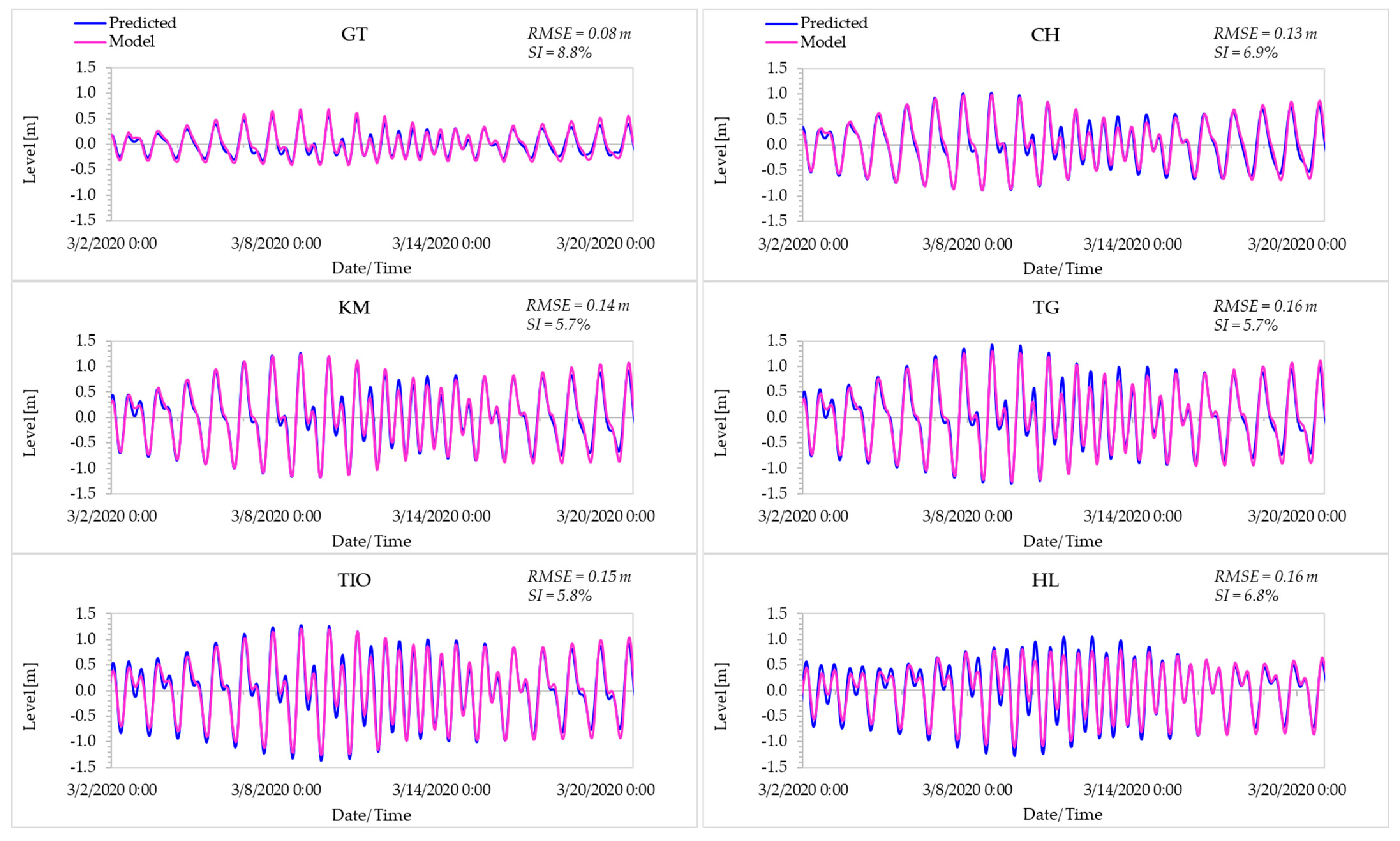
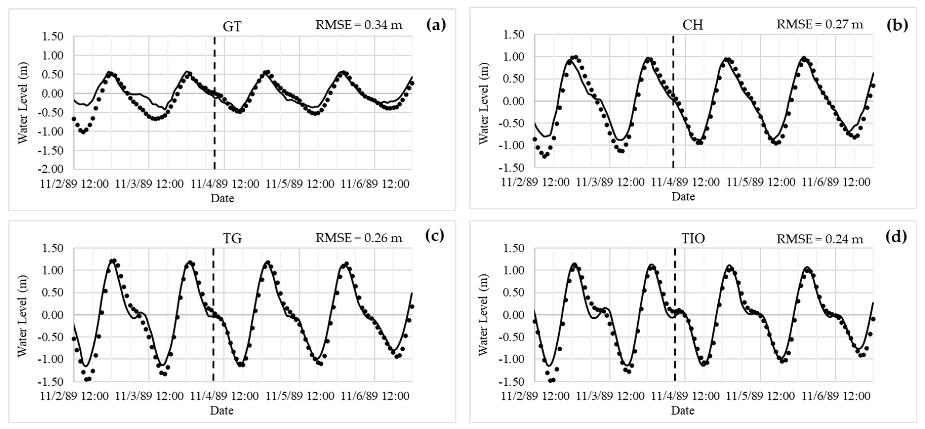
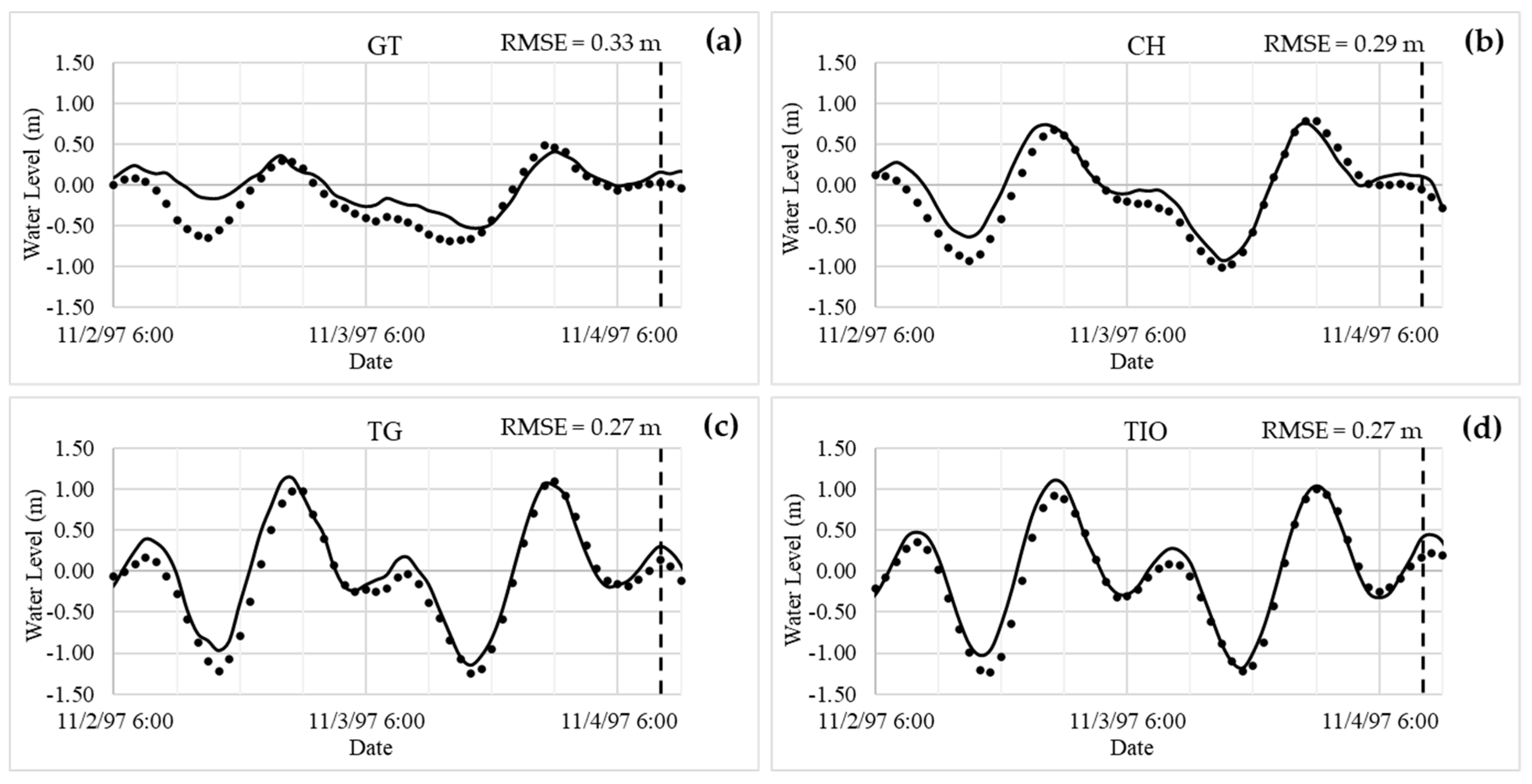
2.5. Water Level Calibration and Validation

To ensure the hydrodynamic and tropical cyclone models used in this study are accurate with reasonable interpretation, model calibration and validation are required. First, the hydrodynamic model for this study was calibrated with the predicted water level at six stations under a non-TC condition (tide only). The accuracy and the reliability of the hydrodynamic and storm model were tested using two statistics, the root-mean-square error (RMSE) and Scatter Index (SI) of the water level data. The RMSE is calculated using Equation (7) and the SI is shown in Equation (8), given below:
R M S E = 1 N 1 n d i f 2 i
S I = R M S m e m a x i m u m   r a n g e * 100
where mei is the measured water level, moi is the modeled water level, and difimoimei, is the difference between the modeled and the measured water levels. The RMSE and SI applied in this study are in accord with the limitation set forth in the Department of Irrigation and Drainage (DID) Guidelines for Coastal Hydraulic Study [81]. However, DID do not explicitly specify the acceptable limits for RMSE and SI for extreme scenarios like storm occurrences, thus, this study applies a general accuracy criterion of 0.3 m and 30% for RMSE and SI, respectively.
Based on Figure 8, the time-series graphs for the Geting (GT), Chendering, (CH), Tg. Gelang (TG), Kemaman (KM), and Tioman (TIO) stations demonstrate good agreement and fall within the DID’s standard of accuracy for the RMSE (<0.2 m) and with SI < 10% for the non-TC or normal tide case [81]. The model accurately reproduces the time variability of the water levels, and the simulated water levels during the spring and neap periods show similarity between the predictions. An overall comparison with the offshore station, HL, shows relatively good agreement with the phase of the tide signal, though the water level during spring tide was underestimated, mainly due to the dynamic of tidal forcing between the island of Pedra Bianca and the Middle Rocks. Nevertheless, the RMSE for HL is 0.16 m and the SI is 6.8%, which are in good agreement with the predicted water level. It is concluded that the RMSE values for all stations were relatively less than 0.2 m and the SI values were less than 10%. The designed model can simulate the influence of various TC parameters on storm surge dynamics well.
Second, the validation process for the storm tide model involved comparing the water levels generated by the model with actual water levels observed during three distinct storm events: Typhoon Gay, STS Linda, and TD 29W. For Typhoon Gay and STS Linda, the model was validated against observed water levels from the stations GT, CH, TG, and TIO. In the case of the TD 29W storm, the observed water levels at KM and TG were used for the comparison. As depicted in Figure 9, the magnitude and fluctuation patterns of the water level during Typhoon Gay show good agreement with the observed water level except for station GT. The model overestimated the water level at station GT with an RMSE of 0.34 m, although the SI value was 29%, which is below the 30% limit. However, the model exhibited a tendency to overestimate the water level in the early stage but performed comparatively well from landfall until the end of the typhoon, as shown in Figure 9a. The stations CH, TG, and TIO displayed good agreement with the observed water level, with RMSE and SI values of less than 0.30 m and below 15%, respectively.
Similarly, the comparison of the modeled water levels during STS Linda (Figure 10) also showed good agreement with the observed water levels for all stations. The SI results for the stations GT, CH, TG, and TIO were 21.7%, 13.2%, 10.1%, and 10.1%, respectively. During TD 29W, the simulated water level at the nearest stations, Kemaman and TG, matched well with the observed water levels, resulting in SI values of 14.1% and 14.3%, respectively (Figure 11). Furthermore, during TD 29W, there was significant storm rainfall accompanying it, which likely influenced the nearshore water levels. However, the simulation could not account for the combined effects of rainfall and the tropical cyclone, leading to a lower simulated surge residual. It is important to note that the entire model simulation occurred during the Northeast Monsoon (NEM) season (November to March), during which monsoon winds can also cause fluctuations in the water surface level. However, this study did not delve into identifying the specific environmental factors contributing to peak surges, leaving it as an intriguing area for future research. In conclusion, the model results agreed well with the observations during three typhoon processes (Gay, Linda, and TD 29W), indicating that the parameters used in the model are appropriate and the model is reasonable for simulating storm surges. Thus, a solid foundation is laid for the development of the next synthetic tropical cyclone model.

3. Results and Discussion

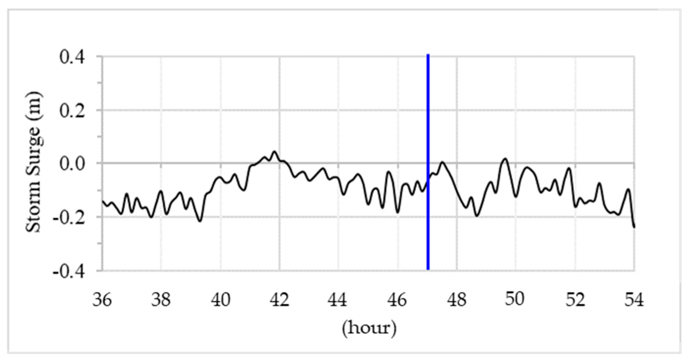
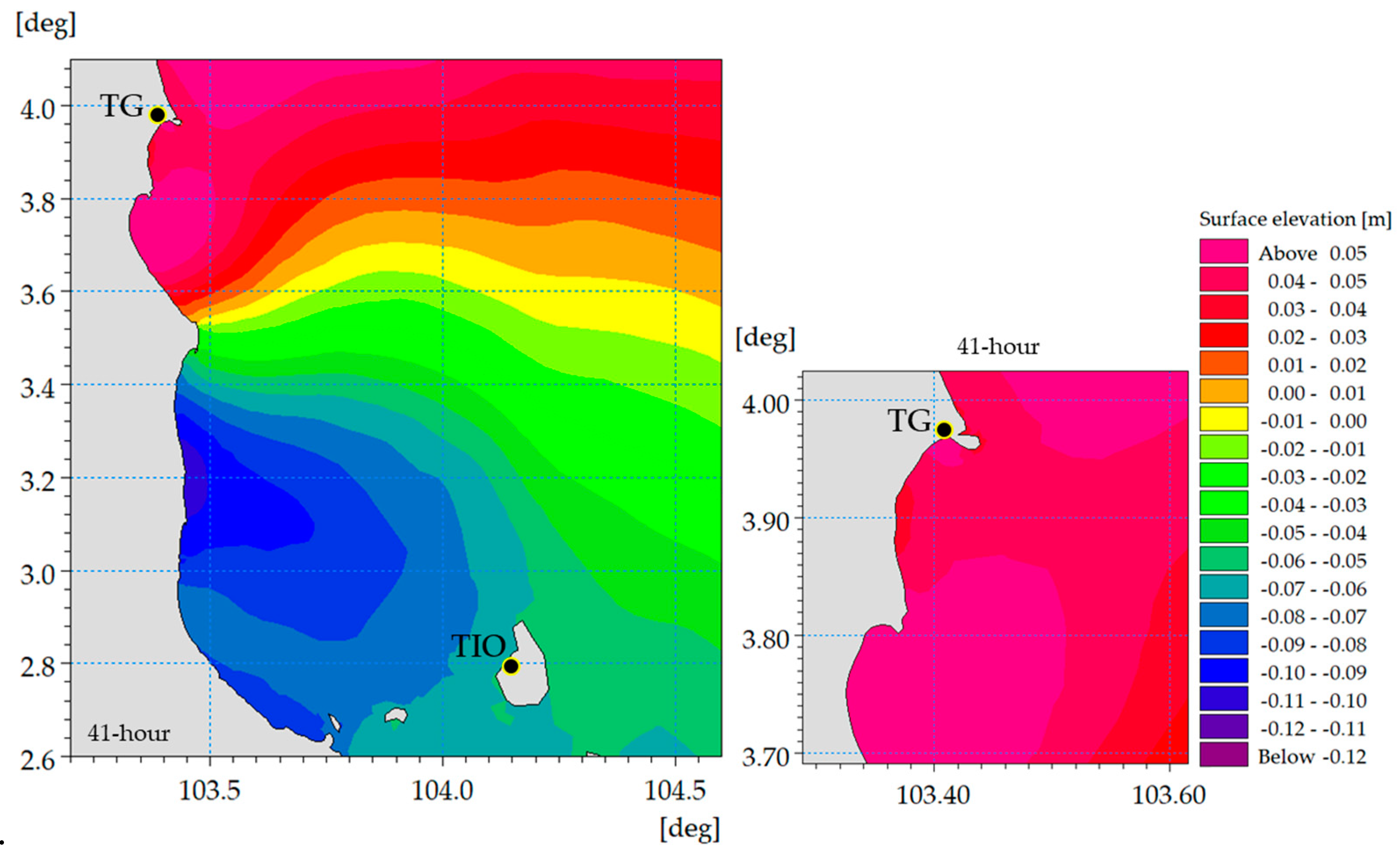
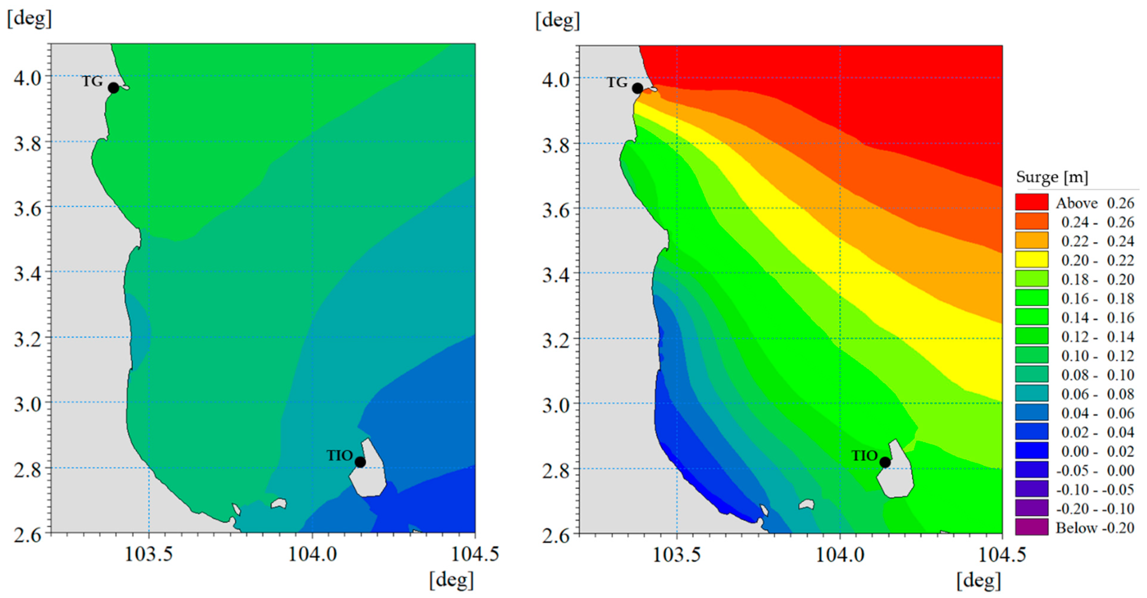
3.1. Storm Surge during TD 29W

The simulation of TD 29W reveals dynamic fluctuations in storm surge over the course of 54 h. This surge, which is calculated by subtracting the astronomical tide from the total water level, exhibits temporal variations along the ECPM coastline. At the moment of typhoon landfall, which occurred at 23:00 UTC on 16 December 2021, storm surge levels along the ECPM coastline varied from −0.16 m near GT to 0.01 m near TIO (refer to Figure 12). During the ebb stage of the tide, the surge residual tended to be slightly positive. The surge hydrograph reflects an N-shaped surge pattern, with a negative surge followed by a positive surge, which is particularly noticeable at GT and CH stations. In contrast, the surge curves at TG and TIO show abrupt changes in the sea level rather than the gradual changes observed in the mirrored N-shaped surge at GT and CH. This suggests that wind setup is the predominant factor driving this phenomenon, which aligns with the findings of [9].
The surge residuals exhibit a pattern in which they are generally less than 0.1 m in the case of TIO but negative when it comes to GT, CH, and TG during the passage of TD 29W. As illustrated in Figure 12, the storm surge displays oscillations that follow the tidal period, demonstrating an inverse relationship with tide elevation. This means that the surge is lower during high tide and higher during low tide, a phenomenon consistent with the observed surge residuals. This reaffirms that the interaction between tides and surges is an unavoidable factor in coastal regions with shallow water depths. This non-linear interplay between tides and surges has a substantial impact on both the amplitude and phase of the surges, especially when TC landfall occurs during spring high tide. The statement is further elaborated in the landfall sensitivity test section. Furthermore, in their study, the authors of [82] indicate that in the region of the Gulf of Thailand and the ECPM, the influence of tide on surge is less significant, which concurs with the findings from this study.
A positive peak surge is evident during the initial 24 h of the typhoon’s path, with fluctuations occurring as the tide rises and gradually recedes toward the conclusion of the typhoon system. The combined effects of the storm surge and tides along the ECPM coastline influence the storm residual, particularly during neap tide. Interestingly, similar effects can be observed during spring tide, as reported in [50]. To delve deeper into the impact of tides on surges during spring tidal periods, further examinations were conducted in subsequent sensitivity tests.
As reported in [46], the angle between the coastline and the direction of the typhoon’s movement plays a pivotal role in determining the maximum surge. A reduction in this angle results in higher surges, particularly in bays and along open coasts. Despite the East Coast of Peninsular Malaysia (ECPM) having a lengthy, open coastline on a continental shelf, during the passage of a typhoon, the water moving toward the shore may have dispersed to both the left and right of the storm’s center, leading to lower surge levels. A similar phenomenon was observed at TG, even though this station is positioned closer to the top right quadrant of the wind movement, where the most intense winds are generated, and higher surges would be expected. Contrary to expectations, a reverse pattern was identified, possibly attributed to the station’s location at a headland, resulting in a relatively modest surge increase, albeit for a short duration (refer to Figure 13). The spatial distribution of maximum surge residuals in the Pahang region during TD 29W is depicted in Figure 14 and Figure 15. From Figure 14, the maximum surge residual in TG occurred 6 h before TC landfall, while at TIO, the maximum surge residual occurred at TC landfall, as shown in Figure 15.
Additionally, the direction of the typhoon’s movement and landfall plays a role in surge magnitude. TD 29W’s landfall location is significantly distant from the stations GT, CH, and TIO. Consequently, far-reaching stations at distances greater than the size of the wind radius tend to experience lower surges. Furthermore, a significant stretch of mangroves lines the coast south of GT station, acting as a coastal barrier and mitigating surge incidents. Conversely, at CH, a series of offshore islands dot the southern coast, indirectly dampening the surge impact induced by TD 29W. TIO station is located even further south from the typhoon’s path, likely experiencing a lower surge impact.
The interaction of tides and surges can lead to increased overall water levels, especially in regions characterized by significant tidal ranges, with some studies proposing that maximum surges are more prone to happening during incoming or outgoing tide rather than during periods of minimal water movement, owing to this dynamic interconnection [48]. However, recent scientific insights emphasize that storm surges are influenced by the unique characteristics of coastal areas, including local atmospheric conditions and coastal geography. In this study, the selected stations have relatively lower tidal ranges compared to stations along the Strait of Malacca (SM). The bottleneck and funnel shape of the SM between the west coast of PM and Sumatera Island can result in higher tidal ranges, as observed in Port Klang with a tidal range exceeding 5.0 m. In contrast, tidal ranges for stations along the ECPM range from 1.0 m at GT to 3.0 m at TG station, which are considered low. Combined with the low intensity of the typhoon (tropical depression) and the long, open coastline, this leads to less pronounced surges.
Additionally, TD 29W coincided with a neap tidal period, resulting in an initial surge level that lacked the significance needed for sustained or continuous intensification (positive surge) until landfall, as illustrated in Figure 16. As a result, we conducted experiments to examine the influence of tidal phase on surge levels at the time of typhoon landfall, specifically comparing neap and spring tidal periods. The outcomes of these investigations are presented in detail in the subsequent section.

3.2. Sensitivity Test on Storm Tide Model

In this section, we explore how various parameters related to tropical cyclones (TCs) impact the height of storm surges. These parameters encompass factors such as the timing of TC landfall, tidal phases, maximum wind speed (intensity), different TC tracks, and sea level rise. To assess the influence of TC landfall timing, we conducted tests at four different time points during the neap tidal period, ranging from 12 h before to 12 h after the initial moment when TD 29W made landfall (refer to Figure 16). Furthermore, experiments were carried out to investigate the effect of TC systems generated during the spring tidal phase on surge height, and this was tested at four distinct time intervals (Figure 16). Throughout the sensitivity tests examining the impact on surge–tide interactions and surge residuals, we specifically focus on presenting and discussing the results obtained from TG and TIO stations, which are the two stations closest to the location of the typhoon’s landfall in the Pahang region.
It is important to note that the storm surge model utilized in this study excludes the consideration of waves and/or rainfall (synonymous with Northeast Monsoon period climate conditions) in all simulations.

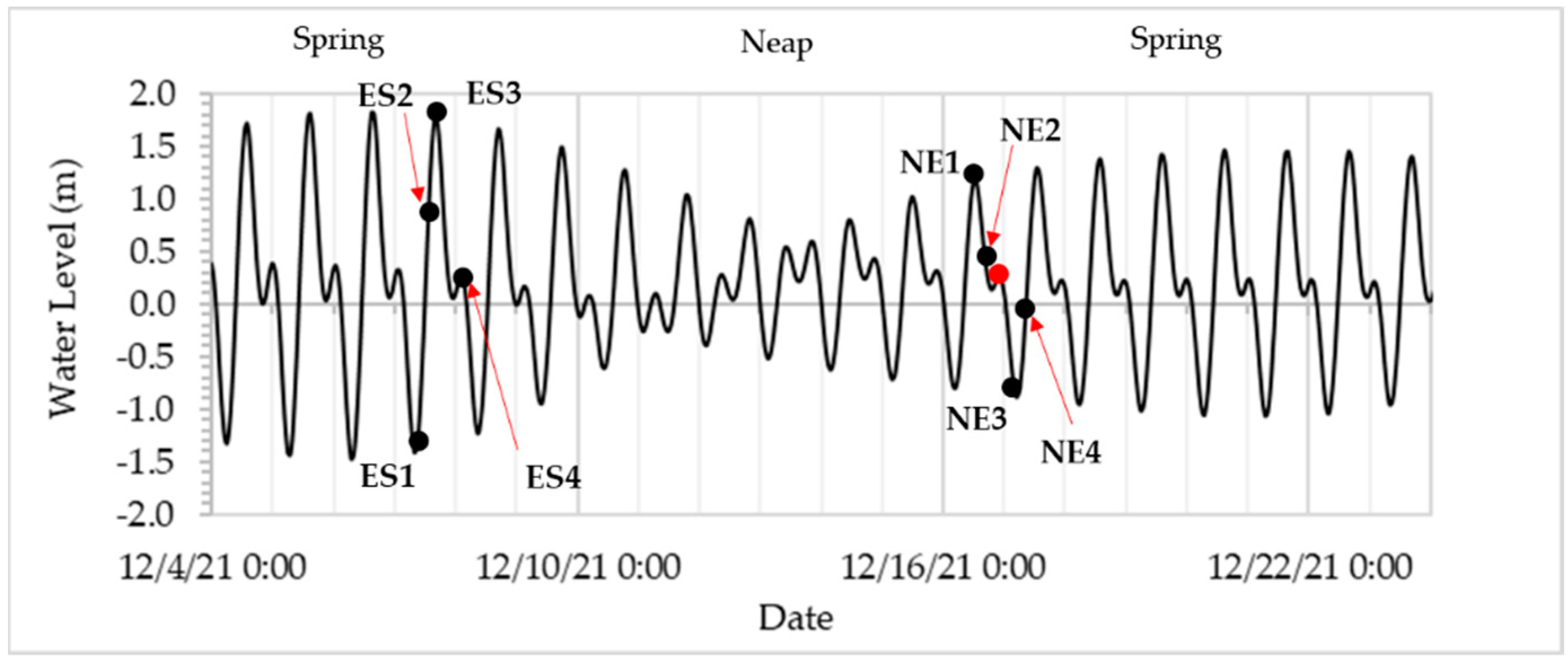
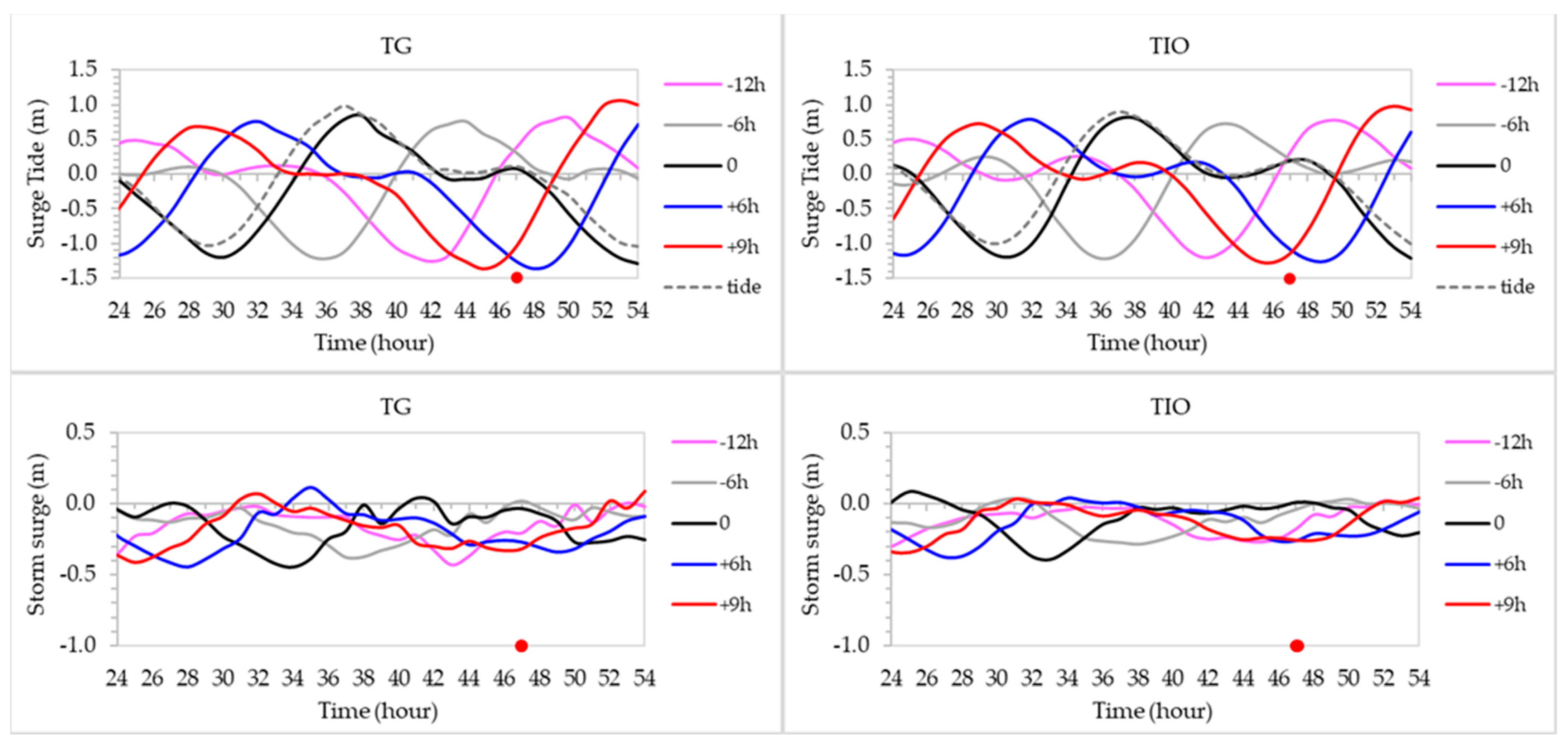
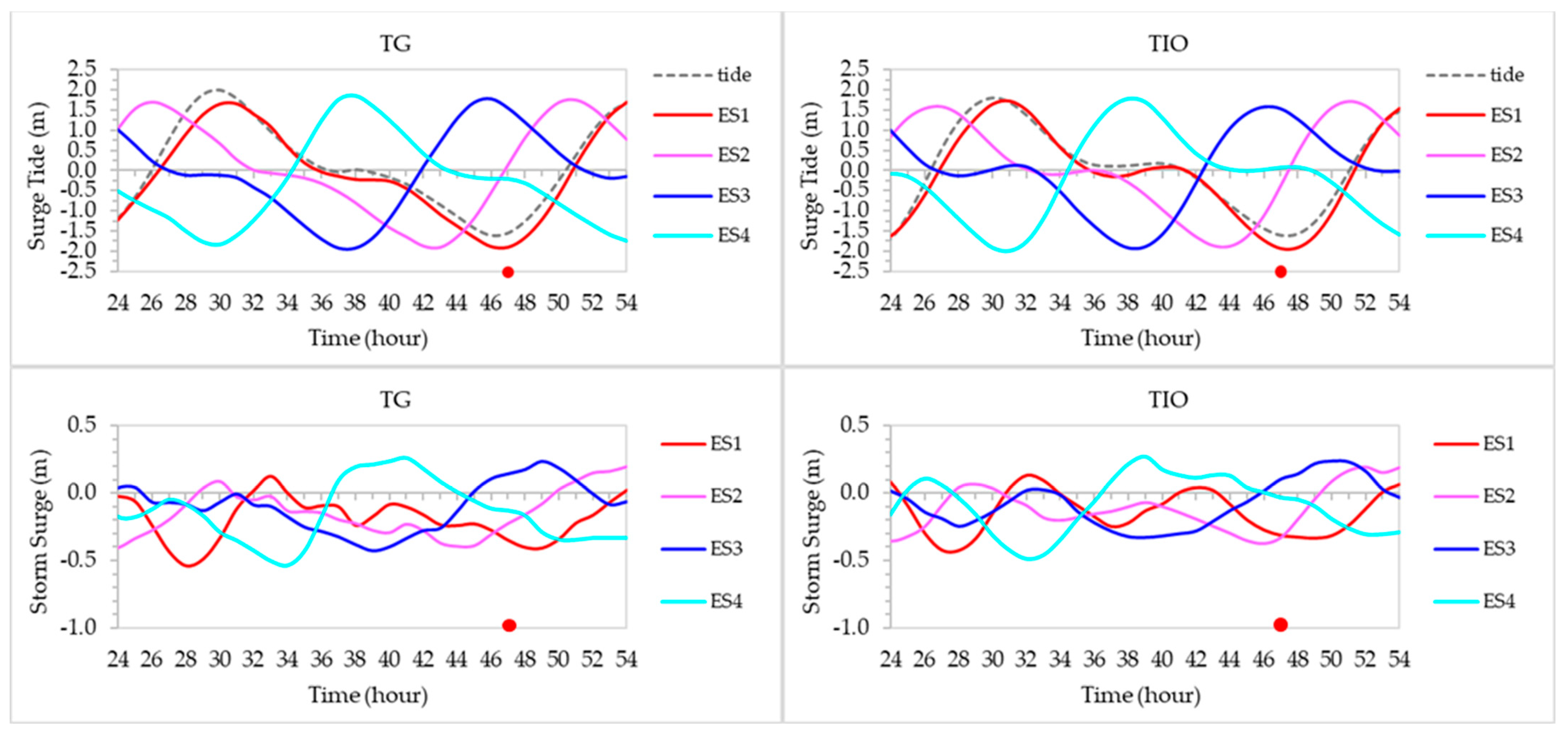
3.2.1. Effect of Landfall Time

This section focuses on assessing the impact of varying landfall timing on induced surges during different phases of the tidal cycle within both neap and spring tidal periods. To examine how these different landfall timings affect storm surges, four simulations for each of these tidal periods were conducted. These simulations utilized tidal forcing with the wind parameters of TD 29W and its typhoon track. Specifically, we considered four-time scenarios: −12 h, −6 h, +6 h, and +9 h relative to the actual typhoon landfall time. These time scenarios corresponded to landfalls occurring at high tide (NE1), ebb tide (NE2), low tide (NE3), and rising tide (NE4), respectively. A negative sign denotes that the landfall timing precedes the actual TD 29W landfall time, while a positive sign indicates a timing after the actual typhoon landfall. During the spring tidal period, four categories of tidal phases were considered, known as ES1, ES2, ES3, and ES4, each associated with low tide, rising tide, high tide, and ebbing tide, respectively (see Figure 16).
Figure 17 and Figure 18 provide a visual representation of the surge tide levels (upper) and surge residuals (lower) under varying landfall timing scenarios during both neap and spring tidal periods, respectively. In Figure 17, the actual typhoon landfall occurred on 16 December 2021 at 23:00 h during neap tide near TG station. This resulted in a surge tide of 0.08 m and 0.19 m, as well as a surge residual of −0.03 m and 0.01 m at TG and TIO, respectively. For the NE1 and NE2 scenarios, the landfall timing was adjusted to coincide with the rising tide (RT) and ebbing tide (ET) on the same day. This led to surge tides of 0.40 m and 0.29 m at TG and 0.18 m (both at RT and ET) at TIO, respectively. In the NE3 and NE4 scenarios, the landfall occurred almost at low tide (LT) for the NE3 case and just as the tide began to rise for NE4 at both TG and TIO. These tests resulted in surge tides of −1.26 m and −1.02 m at TG and −1.09 m and −1.15 m at TIO, respectively. The surge tide fluctuations follow an astronomical tide pattern with a distinct N-shaped pattern observed in all tidal phase tests. The changes in surge height, whether positive or negative, align with previous research findings [28]. Ref. [28] indicates that the change in coastal topography can affect the increase and decrease in positive and negative surges.
However, the negative surge dominates over the positive surge at both TG and TIO stations across all tidal phases tested. The maximum positive surge at TIO occurs at NE4 during a 32 h ebbing tide and later at the end of the typhoon system, resulting in a surge residual of less than 0.1 m at both TG and TIO. In contrast, other tidal phases induce a negative surge at the end of the typhoon system. The prevalence of high negative surges may be attributed to the open coastal areas near TG station, where such open coasts tend to moderate surge heights. On the other hand, TIO station is situated on the lee side of Tioman Island, facing the mainland, and the channel effect has less influence on surge height, leading to a surge residual pattern that closely mirrors that of TG (refer to Figure 17). The relatively greater distance of TIO from the typhoon’s landfall location likely contributes to these lower surge phenomena.
In Figure 18, tests during the spring tidal period indicate similar water level fluctuation as in the neap period for all tidal phases at both TG and TIO. The signature of spring tides is predominantly observed in higher water levels compared to neap tides. Surge tide values of −1.89 m, 0.15 m, 1.54 m, and −0.21 m is observed at the ES1, ES2, ES3, and ES4 landfall timings at TG station, respectively, while at TIO, the surge tide values are −1.92 m, −0.36 m, 1.51 m, and 0.06 m under similar landfall timings, respectively. The positive and negative surge tides during spring tides are quite high.
The peak surge residual prior to landfall timing is observed during the ebbing tide of ES4 with surge heights of 0.26 m and 0.27 m at TG (6 h) and TIO (7 h), respectively, while after typhoon landfall, a peak surge is observed at tidal phase ES3, with surge residuals at TG and TIO of 0.23 m (2 h after) and 0.24 m (3 h after) during ebbing tide, respectively. The maximum surge height at the end of the typhoon system occurs during the ebbing tide of tidal phase ES2, with surge residuals of 0.2 m and 0.19 m at TG and TIO, respectively. Thus, it can be concluded that the tide–surge interactions depend predominantly on the landfall timing of a tidal cycle. In all tested landfall timings during neap and spring tides, the peak surge tends to occur during ebbing tides regardless of the tidal phase, which concurs with [83]. Figure 19 shows the spatial maximum surge level pattern along the Pahang region during neap and spring tidal periods.
Furthermore, the negative surge occurred before the peak surge in the early stage of the surge model. This may be explained by a phenomenon of wind-drifting movement during the typhoon’s passage toward the coast, causing the water mass to propagate away from the coast [84]. Another possible reason is that the convex shape of the north-east coast of the ECPM can potentially weaken the retreating sea current force, pushing the water mass away from the coast [9]. As a result, these phenomena may cause a negative surge at the location where the typhoon makes a landfall. In short, the specific shape of the coastline in this area plays a significant role in influencing the behavior of the sea current and the resulting surge during the typhoon’s passage.

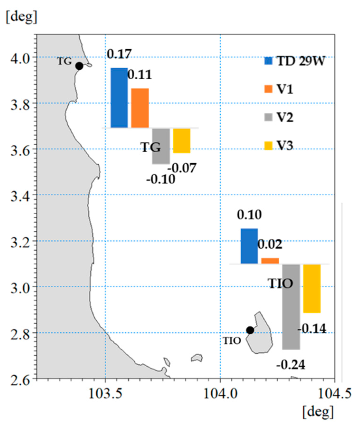
3.2.2. Effect of TC Intensity

In this section, we assess the influence of varying wind intensities on storm surge height. Figure 20 displays the time series of surge residuals at TG and TIO stations during different typhoon wind intensities. Overall, a lower tropical cyclone (TC) intensity resulted in higher positive surge residuals and lower negative surges throughout the typhoon’s progression. There was a descending trend in the surge residuals’ magnitude as the maximum wind speed increased. This wind speed is inversely related to the maximum wind radius (Rmw) of the typhoon, meaning higher wind speeds correspond to smaller Rmw values and vice versa. In this context, V1, V2, and V3 represent tropical storms, severe tropical storms, and typhoon wind parameters, generating larger to smaller Rmw values. As a result, the actual TD 29W had the largest Rmw among the tested wind intensities. These findings regarding positive surges concerning wind intensity align with [28].
Once again, the steep terrain of a headland near TG and the greater distance of TIO from the typhoon’s landfall may have contributed to the occurrence of negative surges. Figure 21 provides a visualization of the maximum surge residuals at various TC intensities.

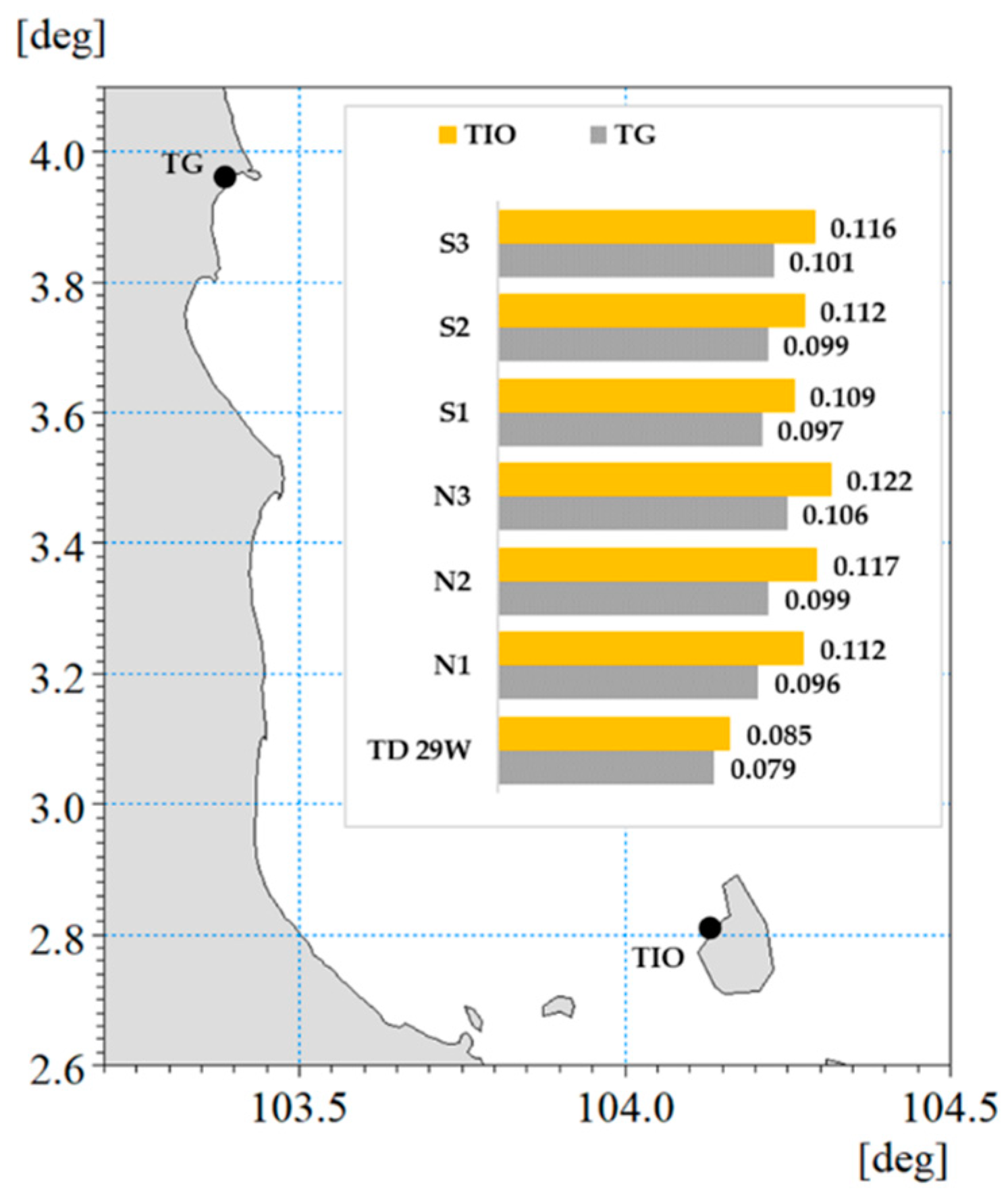
3.2.3. Effect of Typhoon Tracks

Figure 22 presents the time series of surge residuals observed at TG and TIO during simulations of six different typhoon paths. Notably, the surge residual generated by the northward shift track of TD 29W (N3) records the highest values, followed by the southward shift track of TD 29W (S3). At TG, the maximum surge residuals for N3 and S3 are 0.11 m and 0.10 m, respectively, while at TIO, they are both 0.12 m.
Furthermore, in the northward shift tracks (as shown in Figure 22a), the occurrence of positive and negative surges is nearly simultaneous. Conversely, in the southward shift track simulations, there is a slight delay in the case of track S3 (Figure 22b). Surges in N1, N2, and N3 are relatively higher than those observed in the actual typhoon TD 29W, with increases ranging from 16.9% to 30.1%. Similarly, S1, S2, and S3 also result in higher surges than the actual typhoon (TD 29W), with an increment between 18.0% and 26.6%. The authors of [28] previously suggested that the closest typhoon path to the observation point leads to higher surge levels. However, their findings contradict the results of this study, which indicate that the shift in typhoon tracks has a minor impact on surge elevation along the Pahang region.
Another study [85] mentioned that storm surges caused by a typhoon are primarily influenced by the typhoon’s track. Since surges result from wind and pressure fields, the surge level on the open coast at TG is less severe than at TIO. TIO is sandwiched between the mainland PM and Tioman Island, which facilitates water piling up, contributing to the surge in the early stages of the typhoon system. However, the surge level at TIO gradually diminishes as the typhoon system subsides. At TG station, the wind intensity induces a milder positive surge of less than 0.1 m in the initial 30 h, but it rapidly changes to a higher surge before the typhoon’s landfall and then tapers off at the end of the typhoon system. This phenomenon may be attributed to the presence of nearby island archipelagos both north and south of TG station (see Figure 7). The spatial results of the maximum surge residuals under various typhoon tracks, as shown in Figure 23, support this explanation.

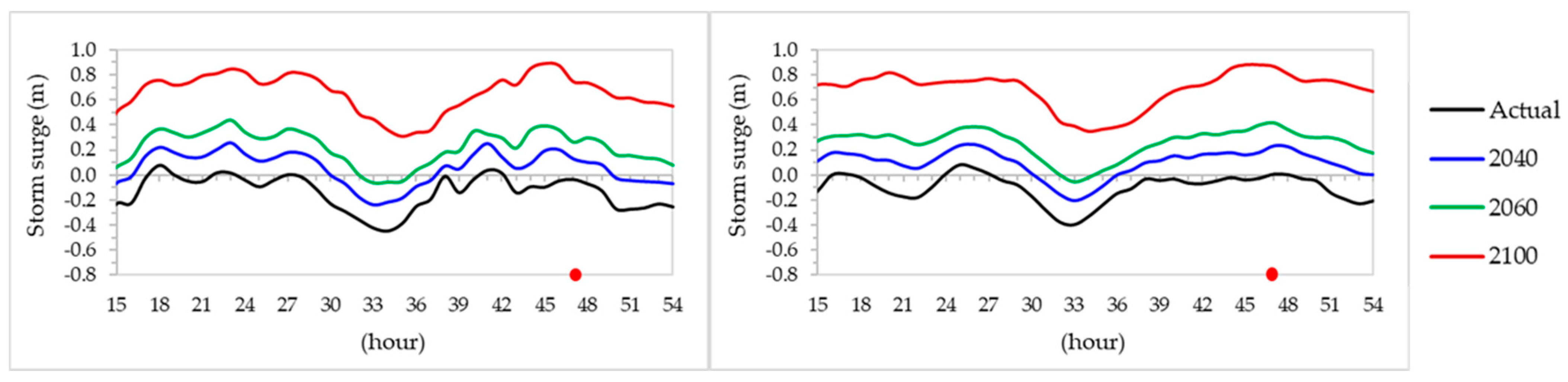
3.2.4. Effect of Sea Level Rise

The storm surge height is expected to increase under the future sea level rise projections (for the years 2040, 2060, and 2100). According to these projections, the anticipated storm surge height in 2040, factoring in the sea level rise at landfall time, is 0.13 m at TG and 0.23 m at TIO. For the years 2060 and 2100, the projected sea level rise results in more substantial storm surge heights of 0.26 m and 0.74 m at TG and 0.42 m and 0.87 m at TIO, respectively (as depicted in Figure 24).
As the storm approaches the shallow nearshore area and prepares to make landfall, the surge in the 2040 sea level rise projection is expected to be particularly significant in comparison to the actual water level (for the year 2021). The storm’s additional energy, due to the higher shear stress on the shallow seabed, contributes to a larger surge. The increased depth resulting from the sea level rise adds further vulnerability to the shoreline. In the case of the 2100 sea level rise projection, there is a severe risk of extensive surge inundation inland. If a major rainstorm coincides with this, the already-inundated inland areas may remain flooded for an extended period. This possibility is based on a historical event during an intense flood that occurred in the northern ECPM states in 2014. With the combined effects of sea level rise and storm surge, the duration of flooding may increase in the future, intensifying the vulnerability to inland flooding. Furthermore, the elevated sea surface due to SLR is likely to shift the peak surge time to an earlier period due to tidal phase shifts and interactions between tides and surges. As shown in Figure 24, the maximum surge height is only 2 h before TC landfall, with surge heights reaching 0.89 m at TG and 0.88 m at TIO in the year 2100. The change in SLR minimally affects the shift in the maximum surge time. The high and low points of the surge almost align with the current surge pattern (induced by TD 29W at the present water level). Figure 25 illustrates the spatial variations in the maximum surge level under various SLR projections.

4. Conclusions

This study examined the impact of tropical-cyclone-induced storm surges in Peninsular Malaysia. It investigated factors such as typhoon paths, tidal phases, wind strength, and the influence of rising sea levels through numerical simulations. The model results closely matched observations for three typhoon events (Typhoon Gay, STS Linda, and TD 29W), demonstrating strong model performance. Most tide gauge stations showed a root-mean-square error (RMSE) of less than 0.30 m and a Scatter Index (SI) of less than 30%.
Research on various tidal conditions revealed differences in surge residuals, emphasizing the importance of tides in storm surge interactions [86,87]. However, local studies on tropical cyclones often overlook this relationship, leading to inaccurate surge height estimates [33,44,56]. The study identified a significant pattern in the timing of peak storm surges. Regardless of landfall times, an N-shaped surge residual pattern was observed. During neap tides, positive peak surges consistently stayed below 0.15 m, matching observed surges. Additionally, the peak surge typically occurred around six hours before or after the actual peak surge of TD 29W, except when typhoons made landfall during rising tides, resulting in a positive surge at the typhoon’s end. Spring tides generated higher positive surge residuals, with peaks during rising, high, and ebbing tides. Importantly, negative surges could occur during rising tides at the time of tropical cyclone landfall, demonstrating the tide–surge interaction rule in which the lowest surge occurs at high tidal levels and vice versa [80].
The study also revealed that an escalation in wind intensity (maximum wind speed) had a limited impact on triggering positive surges. Instead, surge levels diminished as wind intensity increased at both TG and TIO stations, likely due to complex, non-linear interactions between wind dynamics and air pressure which tended to diminish the peak surge heights. However, it is worthwhile to explore in future research the variations in the influence of air pressure on surges. Additionally, this study showed that typhoon paths spanning greater distances had a marginal effect on augmenting surge residuals and modifying the timing of peak surges. The presence of islands to the north and south of TG and TIO stations notably influenced peak surge residuals when typhoons encountered these islands, as evidenced by typhoon tracks N3 and S3.
In future sea-level-rise scenarios, this study projects a concerning increase in storm surge heights along the coastal areas of the ECPM region. According to the scenarios examined, maximum storm surge residuals are expected to rise by 37–69% from the present to 2040 and increase by 22–36% from 2040 to 2100. Sea level rise also influences tidal phase changes, potentially causing earlier peak surge arrivals. Notably, these increases are independent of cyclone wind intensities, indicating that sea level rise itself will significantly contribute to heightened storm surge risks in the future. These findings offer valuable insights for coastal planning and disaster management efforts.

Author Contributions

Conceptualization, methodology, validation, analysis, writing—original draft preparation and editing, and funding acquisition, N.M.A.; writing—review, and supervision, H.-M.T., writing—review, Z.M. All authors have read and agreed to the published version of the manuscript.

Funding

This research received external funding from iCORE PLT for the additional observed data. The publication of this paper was funded by the Murata Science Foundation (21MP04) and YUTP Grant (015LC0-453).

Institutional Review Board Statement

Not applicable.

Informed Consent Statement

Not applicable.

Data Availability Statement

Data are contained within the article.

Acknowledgments

The authors thank IPAKM and DSMM for the provision of the model and the data required for this study, respectively, as well as Siti Habibah Shafiai for her support, encouragement, and insight into the research topic. Additionally, full support from iCORE PLT was provided for the usage of MIKE 21 software for the completion of the TC simulation works.

Conflicts of Interest

The authors declare no conflict of interest. The contributors had no role in the design of the study, collection of data, analyses, or interpretation of data; in the writing of the manuscript, or in the decision to publish the results.

References

  1. Flather, R.A. Storm surges. In Encyclopedia of Ocean Sciences; Steele, J., Thorpe, S., Turekian, K., Eds.; Academic Press: San Diego, CA, USA, 2001; pp. 2882–2892. [Google Scholar]
  2. Intergovernmental Panel on Climate Change (IPCC). Sixth Assessment Report; Cambridge University Press: Cambridge, UK, 2021.
  3. Elsner, J.B.; Liu, K.-B. Examining the ENSO-Typhoon Hypothesis. Clim. Res. 2003, 25, 43–54. [Google Scholar] [CrossRef]
  4. Wittwer, G. Modelling the economic impacts of a significant earthquake in the Perth metropolitan area. In Geoscience Australia Internal Report; Geoscience Australia: Canberra, ACT, Australia, 2004. [Google Scholar]
  5. Rahman, S. Malaysia’s Floods of December 2021: Can Future Disasters Be Avoided? ISEAS Perspective; ISEAS-Yusof Ishak Institute: Singapore, 2022; No. 26. ISSN 2335-6677. [Google Scholar]
  6. Bloemendaal, N.; Haigh, I.D.; de Moel, H.; Muis, S.; Haarsma, R.J.; Aerts, J.C.H. Generation of a global synthetic tropical cyclone hazard dataset using STORM. Sci. Data 2020, 7, 40. [Google Scholar] [CrossRef]
  7. Takahashi, H.G.; Fujinami, H.; Yasunari, T.; Matsumoto, J.; Baimoung, S. Role of tropical cyclone along the Monsoon Trough in the 2011 Thai Flood and Interannual Variability. J. Clim. 2015, 28, 1465–1476. [Google Scholar] [CrossRef]
  8. Wu, L. Possible linkage between the monsoon trough variability and the tropical cyclone activity over the Western North Pacific. Mon. Weather Rev. 2012, 140, 140–150. [Google Scholar] [CrossRef]
  9. Tomkratoke, S.; Sirisup, S. Effects of tropical cyclone paths and shelf bathymetry on inducement of severe storm surges in the Gulf of Thailand. Acta Oceanol. Sin. 2020, 39, 90–102. [Google Scholar] [CrossRef]
  10. Bloemendaal, N.; Muis, S.; Haarsma, R.J.; Verlaan, M.; Apecechea, M.I.; de Moel, H.; Ward, P.J.; Aerts, J.C.J.H. Global modeling tropical cyclone storm surges using high resolution forecasts. Clim. Dyn. 2019, 52, 5031–5044. [Google Scholar] [CrossRef]
  11. World Bank. Malaysia. Available online: nidm.gov.in (accessed on 29 September 2021).
  12. Meteorological Office (MO). UK. Available online: https://www.metoffice.gov.uk/weather (accessed on 17 January 2023).
  13. SEA. Available online: https://www.sea-circular.org/wp-content/uploads/2020/05/SEA-circular-Country-Profile_MALAYSIA.pdf (accessed on 15 October 2023).
  14. Ehsan, S.; Begum, R.A.; Md Nor, N.G.; Abdul Maulud, K.N. Current and potential impacts of sea level rise in the coastal areas of Malaysia. IOP Conf. Ser. Earth Environ. Sci. 2019, 228, 012023. [Google Scholar] [CrossRef]
  15. Ismail, I.; Wong Abdullah, W.S.; Muslim, M.S.M.; Zakaria, R. Physical impact of sea level rise to the coastal zone along the east coast of Peninsular Malaysia. Malays. J. Geosci. MJG 2018, 2, 33–38. [Google Scholar] [CrossRef]
  16. Ariffin, E.H.; Mathew, M.J.; Roslee, A.; Ismailuddin, A.; Lee, S.Y.; Putra, A.B.; Ku Yusif, K.M.K.; Menhat, M.; Ismail, I.; Shamsul, H.A.; et al. A multi-hazards coastal vulnerability index of the east coast of Peninsular Malaysia. Int. J. Disaster Risk Reduct. 2023, 84, 103484. [Google Scholar] [CrossRef]
  17. NAHRIM. Sea-Level Rise Projections for Malaysia; Report Submitted to the National Hydraulic Institute of Malaysia, Ministry of Natural Resources and Environment by California Hydrological Research Laboratory (CHRL); NAHRIM: Seri Kembangan, Malaysia, 2010.
  18. NAHRIM. Impact of Climate Change Sea Level Rise Projections for Malaysia; Minister of Environment and Water (KASA), National Water Research Institute of Malaysia (NAHRIM): Seri Kembangan, Malaysia, 2017; ISBN 978-976-0382-08-1.
  19. Benson, Y.A.; Hasan, M.M.; Jamal, M.H.; Lee, H.L.; Anthony, D.; Mohamad, K.A.; Hamzah, S.B.; Othman, I.K. Erosion-deposition prone assessment along the Kelantan and Terengganu coasts due to sea level rise. IOP Conf. Ser. Earth Environ. Sci. 2023, 1167, 012029. [Google Scholar] [CrossRef]
  20. Mohamad, M.F.; Lee, H.L.; Samion, M.K.H. Coastal vulnerability assessment towards sustainable management of Peninsular Malaysia coastline. Int. J. Environ. Sci. Dev. 2014, 5, 533. [Google Scholar] [CrossRef]
  21. Mohamad, M.F.; Abdul Hamid, M.R.; Awang, N.A.; Mohd Shah, A.; Hamzah, A.F. Impact of sea level rise due to climate change: Case study of Klang and Kuala Langat District. Int. J. Eng. Technol. 2018, 10, 59–65. [Google Scholar] [CrossRef]
  22. Mohd Anuar, N.; Awang, N.A.; Wan Ahmad Azhary, W.A.H.; Abdul Hamid, M.R. Coastal vulnerability indicators in Langkawi Island under sea level rise impact. In Proceedings of the 4th International Conference on Water Resources (ICWR-2018), Langkawi, Malaysia, 27–28 November 2018. [Google Scholar]
  23. Mohd, F.A.; Rahman, A.A.A.; Abdul Maulud, K.N.; Kamarudin, M.K.; Majid, N.A.; Rosli, A. Geospatial approach for coastal vulnerability assessment of Selangor coast, Malaysia. IOP Conf. Ser. Earth Environ. Sci. 2012, 767, 012025. [Google Scholar] [CrossRef]
  24. Mohd Ghazali, N.H.; Awang, N.A.; Mahmud, M.; Mokhtar, A. Impact of sea level rise and tsunami on coastal areas of north-west Peninsular Malaysia. Irrig. Drain. 2018, 67, 119–129. [Google Scholar] [CrossRef]
  25. Bilskie, M.V.; Hagen, S.C.; Alizad, K.; Medeiros, S.C.; Passeri, D.L.; Needham, H.F.; Cox, A. Dynamic simulation and numerical analysis of hurricane storm surge under sea level rise with geomorphologic changes along the northern Gulf of Mexico. Earth’s Future 2016, 4, 177–193. [Google Scholar] [CrossRef]
  26. Wang, Y.; Guo, Z.; Cheng, S.; Zhang, M.; Shu, X.; Luo, J.; Qiu, L.; Gao, T. Risk assessment for typhoon-induced storm surges in Wenchang, Hainan Island of China. Geomat. Nat. Hazards Risk 2021, 12, 880–899. [Google Scholar] [CrossRef]
  27. Ma, Y.; Wu, Y.; Shao, Z.; Cao, T.; Liang, B. Impacts of sea level rise and typhoon intensity on storm surges and waves around the coastal area of Qingbao. Ocean Eng. 2022, 249, 110953. [Google Scholar] [CrossRef]
  28. Chu, D.; Niu, H.; Qiao, W.; Jiao, X.; Zhang, X.; Zhang, J. Modeling study on the asymmetry of positive and negative storm surges along the Southern Coasts of China. J. Mar. Sci. Eng. 2021, 9, 458. [Google Scholar] [CrossRef]
  29. Zhang, M.; Zhou, C.; Zhang, J.; Zhang, X.; Tang, Z. Numerical Simulation and Analysis of Storm Surges Under Different Extreme Weather Event and Typhoon Experiments in the South Yellow Sea. J. Ocean Univ. China 2022, 21, 1–15. [Google Scholar] [CrossRef]
  30. Kyprioti, A.P.; Taflanidis, A.A.; Nadal-Caraballo, N.C.; Campbell, M.O. Incorporation of sea level rise in storm surge surrogate modeling. Nat. Hazards 2021, 105, 531–563. [Google Scholar] [CrossRef]
  31. Abdelhafiz, M.A.; Ellingwood, B.; Mahmoud, H. Vulnerability of seaports to hurricanes and sea level rise in a changing climate: A case study for mobile, AL. Coast. Eng. 2021, 167, 103884. [Google Scholar] [CrossRef]
  32. Kohno, N. JMA International Cooperation in Storm Surge Forecasts in Southeast Asia. In Proceedings of the JMA/WMO Workshop on Effective Tropical Cyclone Warning in Southeast Asia, Tokyo, Japan, 11–14 March 2014. [Google Scholar]
  33. Conctento, A.; Xu, H.; Gardoni, P. Probabilistic formulation for storm surge predictions. Struct. Infrastruct. Eng. 2020, 16, 547–566. [Google Scholar] [CrossRef]
  34. Luettich, R.A.; Westerink, J.J. Formulation and Numerical Implementation of the 2D/3D ADCIRC Finite Element Model Version 44.XX. 2004. Available online: https://adcirc.org/wp-content/uploads/sites/2255/2018/11/2004_Luettich.pdf (accessed on 20 April 2020).
  35. Zhang, Y.; Baptista, A.M. SELFE: A Semi-implicit Eulerian-Lagrangian Finite-element model for cross-scale ocean circulation. Ocean Model. 2008, 21, 71–96. [Google Scholar] [CrossRef]
  36. Soe, M.E.N.; Thant, D.A.A.; Htun, K.Z. Prediction of storm surge and risk assessment of Rakhine Coastal Region. Am. Sci. Res. J. Eng. Technol. Sci. ASRJETS 2018, 41, 162–180. [Google Scholar]
  37. Wu, T.-R.; Tsai, Y.-L.; Terng, C.-T. The recent development of storm surge modelling in Taiwan. Procedia IUTAM 2017, 25, 70–73. [Google Scholar] [CrossRef]
  38. DHI. MIKE 21 HD-FM—Hydrodynamic Module, User Guide, 148; DHI: Hørsholm, Denmark, 2017. [Google Scholar]
  39. Juneng, L.; Tangang, F.T.; Reason, C.J.; Moten, S.; Hassan, W.A.W. Simulation of tropical cyclone Vamei (2001) using the PSU/NCAR MM5 model. Meteorol. Atmos. Phys. 2007, 97, 273–290. [Google Scholar] [CrossRef]
  40. Almar, R.; Ranasinghe, R.; Bergsma, E.W.J.; Diaz, H.; Melet, A.; Papa, F.; Vousdoukas, M.; Athanasiou, P.; Dada, O.; Almeida, L.P.; et al. A global analysis of extreme coastal water levels with implications for potential coastal overtopping. Nat. Commun. 2021, 12, 3775. [Google Scholar] [CrossRef]
  41. Japan Meteorological Agency. RSMC Best Tract Data of the RSMC Tokyo—Typhoon Center. Available online: https://www.jma.go.jp/jma/jma-eng/jma-center/rsmc-hp-pub-eg/besttrack.html (accessed on 21 April 2020).
  42. Al Azad, A.S.M.A.; Mita, K.S.; Zaman, M.W.; Akter, M.; Asik, T.Z.; Haque, A.; Hussain, M.A.; Rahman, M.M. Impact of tidal phase on inundation and thrust force due to storm surge. J. Mar. Sci. Eng. 2018, 6, 110. [Google Scholar] [CrossRef]
  43. Islam, M.R.; Takagi, H. Typhoon parameter sensitivity of storm surge in the semi-enclosed Tokyo Bay. Front. Earth Sci. 2020, 14, 553–567. [Google Scholar] [CrossRef]
  44. Du, M.; Hou, Y.; Hu, P.; Wang, K. Effects of typhoon paths on storm surge and coastal inundation in the Pearl River Estuary, China. Remote Sens. 2020, 12, 1851. [Google Scholar] [CrossRef]
  45. Yin, C.; Zhang, W.; Xiong, M.; Wang, J.; Zhou, C.; Dou, X.; Zhang, J. Storm surge responses to the representative tracks and storm timing in the Yangtze Estuary, China. J. Ocean Eng. 2021, 233, 109020. [Google Scholar] [CrossRef]
  46. Zhang, Z.; Guo, F.; Song, Z.; Chen, P.; Liu, F.; Zhang, D. A numerical study of storm surge behaviour in and around Lingdingyang Bay, Pearl River Estuary, China. Nat. Hazards 2022, 111, 1507–1532. [Google Scholar] [CrossRef]
  47. Prandle, D.; Wolf, J. The interaction of surge and tide in the North Sea and River Thames. Geophys. J. R. Astron. Soc. 1978, 55, 203–216. [Google Scholar] [CrossRef]
  48. Horsburgh, K.J.; Wilson, C. Tide-surge interaction and its role in the distribution of surge residuals in the North Sea. J. Geophys. Res. Ocean 2007, 112, C08003. [Google Scholar] [CrossRef]
  49. Medvedev, I.P.; Rabinovich, A.B.; Sepic, J. Destructive coastal sea level oscillations generated by Typhoon Maysak in the Sea of Japan in September 2020. Sci. Rep. 2022, 12, 8463. [Google Scholar] [CrossRef]
  50. Liu, W.-C.; Huang, W.-C.; Chen, W.-B. The interaction between tides and storm surges for the Taiwan Coast—A modeling investigation. In Proceedings of the 12th International Conference on Hydroscience & Engineering, Hydro-Science & Engineering for Environmental Resilience, Tainan, Taiwan, 6–10 November 2016. [Google Scholar]
  51. Yin, K.; Xu, S.; Huang, W.; Xie, Y. Effects of sea level rise and typhoon intensity on storm surge and waves in Pearl River Estuary. J. Ocean Eng. 2017, 136, 80–93. [Google Scholar] [CrossRef]
  52. Lin, M.-Y.; Sun, W.-Y.; Chiou, M.-D.; Chen, C.-Y.; Cheng, H.-Y.; Chen, C.-H. Development and evaluation of a storm surge warning system in Taiwan. Ocean Dyn. 2018, 68, 1025–1049. [Google Scholar] [CrossRef]
  53. Jinshan, Z.; Weisheng, Z.; Jun, Z.; Jinhua, W.; Xiong, M.; Chentuan, Y. Characteristics of storm surge due to typical typhoon tracks in coastal areas of the South Yellow Sea. In Proceedings of the APAC 2019 10th International Conference on Asian and Pacific Coasts, Hanoi, Vietnam, 25–28 September 2019; pp. 21–26. [Google Scholar]
  54. Yuxing, W.; Ting, G.; Ning, J.; Zhenyu, H. Numerical study of the impacts of typhoon parameters on the storm surge based on Hato storm over the Pearl River Mouth, China. J. Reg. Stud. Mar. Sci. 2020, 34, 101061. [Google Scholar] [CrossRef]
  55. Hong Kong Observatory. Available online: https://www.hko.gov.hk/informtc/tcReporte.htm (accessed on 21 April 2021).
  56. Loy, K.C.; Koh, H.L.; Liew, J.; Tangang, F. Simulation of circulation and storm surge in South China Sea. In Proceedings of the International Conference on Environment, Penang, Malaysia, 13–15 November 2006. [Google Scholar]
  57. Sinha, P.C.; Jain, I.; Husain, M.L.; Mohd Shazili, N.A.; Choon, L.K. Storm Surge Estimation Along the Coasts of Peninsular Malaysia Using Idealised Typhoons. J. Sustain. Sci. Manag. 2009, 4, 9–17. [Google Scholar]
  58. Morin, V.; Warnitchai, P.; Weesakul, S. Storm surge hazard in Manila Bay: Typhoon Nesat (Pedring) and the SW monsoon. Nat. Hazards 2016, 81, 1569–1588. [Google Scholar] [CrossRef]
  59. Pan, Z.; Liu, H. Numerical study of typhoon-induced storm surge in the Yangtze Estuary of China using a coupled 3D model. Procedia Eng. 2015, 116, 849–854. [Google Scholar] [CrossRef]
  60. Dong, S.; Stephenson, W.J.; Wakes, S.; Chen, Z.; Ge, J. Meso-scale of typhoon generated storm surge: Methodology and Shanghai case study. Nat. Hazards Earth Syst. Sci. Discuss. 2017, 34, 1–18. [Google Scholar] [CrossRef]
  61. Sarker, S.A. Numerical Modeling of Storm Surge from the 1991 Cyclone in the Bay of Bengal (Bangladesh) by Royal Haskoning DHV. J. Environ. Sci. Allied Res. 2019, 3, 8. [Google Scholar]
  62. DID. Integrated Shoreline Management Plan (ISMP) for South Pahang Mainland; Report Prepared by JK Bersatu Sdn Bhd for Department of Irrigation and Drainage Malaysia; Department of Irrigation & Drainage Malaysia: Kuala Lumpur, Malaysia, 2006.
  63. Mohd Anuar, N.; Hashim, A.M.; Awang, N.A.; Abd Hamid, M.R. Historical storm surges: Consequences on coastal resources and shoreline protection in East Coast of Peninsular Malaysia. In Proceedings of the 7th IAHR International Symposium on Hydraulic Structures, Aachen, Germany, 15–18 May 2018. [Google Scholar] [CrossRef]
  64. Mohd, F.A.; Abdul Maulud, K.N.; Abdul Karim, O.; Begum, R.A.; Awang, N.A.; Abdul Hamid, M.R.; Abd Rahim, N.A.; Abd Razak, A.H. Assessment of coastal inundation of low lying areas due to sea level rise. IOP Conf. Ser. Earth Environ. Sci. 2018, 169, 012046. [Google Scholar] [CrossRef]
  65. Van Marren, D.S.; Gerritsen, H. Residual flow and tidal asymmetry in the Singapore Strait, with implications for resuspension and residual transport of sediment. J. Geophys. Res. 2012, 117, C04021. [Google Scholar] [CrossRef]
  66. Matthew, A.; Lekshmy Devi, C.A. Assessing the Impact of Storm Surges in Coastal Regions by Integrating Hydrodynamic and Wave Model with GIS; Preprint from Research Square. 2023; PPR:PPR592592. Available online: https://doi.org/10.21203/rs.3.rs-2332688/v1 (accessed on 20 September 2023).
  67. Nahiduzzaman, S. Simulation of Storm Surge Level at a Tidal Channel due to Coastal Cyclone along the Bangladesh Coast. Master’s Thesis, Bangladesh University of Engineering and Technology, Dhaka, Bangladesh, 2018. [Google Scholar]
  68. Smagorinsky, J. General circulation experiments with the primitive equations. Mon. Weather Rev. 1963, 91, 64–99. [Google Scholar] [CrossRef]
  69. Zarzycki, C.M. Sowing storms: How model timestep can control tropical cyclone in a GCM. J. Adv. Model. Earth Syst. 2022, 14, e2021MS002791. [Google Scholar] [CrossRef]
  70. Zhang, W.-Z.; Lin, S.; Jiang, X.-M. Influence of tropical cyclones in the Western North Pacific. In Recent Developments in Tropical Cyclone Dynamics, Prediction, and Detection; InTech: Wellington, New Zealand, 2016. [Google Scholar] [CrossRef]
  71. DHI. MIKE 21—Cyclone Wind Generation Tool, User Guide, 10; DHI: Hørsholm, Denmark, 2017. [Google Scholar]
  72. Savioli, J.; Pedersen, C.; Szylkarski, S.; Kerper, D. Modelling the Threat of Tropical Cyclone Storm Tide to the Burdekin Shire, Queensland Australia. 2003. Available online: https://mssanz.org.au/MODSIM03/Volume_02/A12/03_Savioli.pdf (accessed on 9 September 2023).
  73. Young, I.R.; Sobey, R.J. The Numerical Prediction of Tropical Cyclone Wind-Waves; James Cook University of North Queensland, Department of Civil & Systems Engineering: Townsville, QLD, Australia, 1981; Research Bulletin No. CS20. [Google Scholar]
  74. Takagi, H.; Wu, W. Maximum Wind Radius Estimated by the 50 kt Radius: Improvement of Storm Surge Forecasting over the Western North Pacific. Nat. Hazards Earth Syst. Sci. 2016, 16, 705–717. [Google Scholar] [CrossRef]
  75. Takagi, H.; Thao, N.D.; Esteban, M.; Tam, T.T.; Knaepen, H.L.; Mikami, T. Vulnerability of coastal areas in Southern Vietnam against tropical cyclones and storm surges. In Proceedings of the International Conference on Estuaries and Coasts, Hanoi, Vietnam, 8–11 October 2012. [Google Scholar]
  76. Quiring, S.; Schumacher, A.; Labosier, C.; Zhu, L. Variations in Mean Annual Tropical Cyclone Size in the Atlantic. J. Geophys. Res. 2011, 116, D09114. [Google Scholar] [CrossRef]
  77. Willoughby, H.E.; Rahn, M.E. Parametric Representation of the Primary Hurricane Vortex. Part I: Observations and Evaluation of the Holland (1980) Model. Mon. Weather Rev. 2004, 132, 3022–3048. [Google Scholar] [CrossRef]
  78. Ott, S. Extremes Winds in the Northern West Pacific; Risø National Laboratory Report Risø-R-1544 (EN). Available online: chrome-extension://efaidnbmnnnibpcajpcglclefindmkaj/https://orbit.dtu.dk/files/7703375/ris_r_1544.pdf (accessed on 14 May 2021).
  79. Harper, B.A.; Holland, G. An Updated Parametric Model of the Tropical Cyclone. In Proceedings of the AMS 23rd Conference on Hurricanes and Tropical Meteorology, Dallas, TX, USA, 11–15 January 1999. [Google Scholar]
  80. Sobey, R.J.; Harper, B.A.; Stark, K.P. Numerical Simulation of Tropical Cyclone Storm Surge; James Cook University of North Queensland, Department of Civil & Systems Engineering: Townsville, QLD, Australia, 1977; Research Bulletin No. CS14. [Google Scholar]
  81. DID. Guidelines for Preparation of Coastal Engineering Hydraulic Study and Impact Evaluation; Jabatan Pengairan dan Saliran (JPS): Kuala Lumpur, Malaysia, 2013.
  82. Tomkratoke, S.; Sirisup, S.; Udomchoke, V.; Kanasut, J. Influence of resonance on tide and storm surge in the Gulf of Thailand. Cont. Shelf Res. 2015, 109, 112–116. [Google Scholar] [CrossRef]
  83. Zhang, W.-Z.; Shi, F.; Hong, H.-S.; Shang, S.-P.; Kirby, J.T. Tide-surge Interaction Intensified by the Taiwan Strait. J. Geophys. Res. Oceans 2010, 115, C06012. [Google Scholar] [CrossRef]
  84. Tomkratoke, S.; Sirisup, S.; Vannarut, S.; Udomchoke, V. Effects of tropical storm on storm surge in the Gulf of Thailand: A numerical study. In Proceedings of the 51st Kasetsart University Annual Conference, Bangkok, Thailand, 5–7 February 2013. [Google Scholar]
  85. Rego, J.L.; Li, C. Nonlinear Terms in Storm Surge Predictions: Effect of Tide Anf Shelf Geometry with Case Study from Hurricane Rita. J. Geophys. Res. 2010, 115, C06020. [Google Scholar] [CrossRef]
  86. Antony, C.; Unnikrishnan, A.S.; Krien, Y.; Murty, P.L.N.; Samiksha, S.V.; Islam, A.K.M.S. Tide-surge interaction at the head of the Bay of Bengal during Cyclone Aila. J. Reg. Stud. Mar. Sci. 2020, 35, 101133. [Google Scholar] [CrossRef]
  87. He, Z.; Tang, Y.; Xia, Y.; Chen, B. Interaction impacts of tides, waves and winds on storm surge in a channel-island system: Observational and numerical study in Tangshan Harbor. J. Ocean Dyn. 2020, 70, 307–325. [Google Scholar] [CrossRef]
Figure 1. Storm surge risk in Southeast Asia. JMA Typhoon Centre jurisdiction (blue area) [32,41].
Jmse 11 02223 g001
Figure 2. Study area. (a) of the East Coast of Peninsular Malaysia; (b) Model domain. The black dots are the selected tide gauges for the study.
Jmse 11 02223 g002
Figure 3. Typhoon paths were used in the research calibration and validation processes. For the examination of tropical cyclone wind intensity, TD 29W (magenta line), Typhoon Muifa (yellow line), and Tropical Storm Sonamu (cyan line) were employed.
Jmse 11 02223 g003
Figure 4. Mesh model (top) and the final model bathymetry (bottom). The top-right corner features a magnified mesh view of sections of the ECPM region.
Jmse 11 02223 g004
Figure 5. Bathymetry model. The black dots indicate the TG and TIO standard tide stations in Pahang and Kuantan is the state capital of Pahang.
Jmse 11 02223 g005
Figure 6. Wind speed (left) and pressure (right) for Ty Gay (top) and TD 29W (bottom) at landfall.
Jmse 11 02223 g006
Figure 7. TC track of TD 29W (red line, 0o) and the hypothetical TC tracks.
Jmse 11 02223 g007
Figure 8. Time series of the water level in (m) at a standard tide station in a non-TC simulation. Model (magenta) and predicted (blue) water levels. The RMSE values for each station are well within 10% of the SI (DID’s limit for the normal tide/non-TC case).
Jmse 11 02223 g008
Figure 9. Comparison of model results (dots) with observed (line) at four selected tide gauge stations, (a) GT, (b) CH, (c) TG, and (d) TIO, for four days of Ty Gay at local time. Time of typhoon landfall (4 November 1989 00:00 UTC) shown as a vertical black line.
Jmse 11 02223 g009
Figure 10. Comparison of the model’s results (dots) with observed values (line) at four selected tide gauge stations, (a) GT, (b) CH, (c) TG, and (d) TIO, for four days of STS Linda at local time. Time of typhoon landfall (4 November 1997 00:00 UTC) shown as vertical black line.
Jmse 11 02223 g010
Figure 11. Comparison of the model’s results (dots) with observed values (line) at (a) TG and (b) KM stations during TD 29W. Time of typhoon landfall (16 December 2021 23:00 UTC) shown as vertical black line.
Jmse 11 02223 g011
Figure 12. Storm surge hydrograph during TD 29W at four stations along the coastline of the ECPM. The red line indicates the time of typhoon landfall.
Jmse 11 02223 g012
Figure 13. Observed storm surge residual (m) pattern during TD 29W at TG station. The blue vertical line indicates the typhoon landfall.
Jmse 11 02223 g013
Figure 14. Maximum storm surge residual (m) at TG indicative of surge behavior during TD 29W.
Jmse 11 02223 g014
Figure 15. Maximum storm surge residual (m) at TIO indicative of surge behavior during TD 29W.
Jmse 11 02223 g015
Figure 16. TD 29W occurred during neap tidal period with landfall time of TD 29W (red dot). Test on TC landfall at different tidal phase (black dot).
Jmse 11 02223 g016
Figure 17. Temporal variations in the water level (upper) and storm surge residual (lower) at different tidal phases at TG (left) and TIO (right) during a neap tidal period. The red dot indicates the time of landfall.
Jmse 11 02223 g017
Figure 18. Temporal variations in the water level (upper) and storm surge residual (lower) at different tidal phases at TG (left) and TIO (right) during a spring tidal period. The red dot indicates the time of landfall.
Jmse 11 02223 g018
Figure 19. Spatial distribution of the maximum surge residual (m) along the Pahang region, during LT in the neap (left) tidal period and during ES4 in the spring (right) tidal period.
Jmse 11 02223 g019
Figure 20. Temporal surge patterns at TG (left) and TIO (right) under different TC intensities, V1, V2, and V3. The red dot indicates the TC landfall time.
Jmse 11 02223 g020
Figure 21. Maximum surge level variance under different TC intensities. The black dots indicate the TG and TIO station.
Jmse 11 02223 g021
Figure 22. Storm surge (m) at TG and TIO under different track experiments, (a) northward shift tracks (upper), and (b) southward shift tracks. Red dot indicates the TC landfall time.
Jmse 11 02223 g022
Figure 23. Maximum surge level variance under different TC tracks. The black dots indicate the TG and TIO station.
Jmse 11 02223 g023
Figure 24. Storm surge (m) at TG and TIO, under MSL (black), SLR 2040 (blue), SLR 2060 (green), and SLR 2100 (red). The red dot indicates the TC landfall time.
Jmse 11 02223 g024
Figure 25. Maximum surge level variance under different SLR. The black dots indicate the TG and TIO station.
Jmse 11 02223 g025
Table 1. Best track data for the year 2021 for TD 29W [41].
(yyyymmddhh)Long. (oE)Lat. (oN)Pressure (hPa)Wind (m/s)
2021121500107.75.210087.7
2021121506107.45.0100810.3
2021121512107.14.8100810.3
2021121518106.64.7100710.3
2021121600106.24.7100710.3
2021121606105.14.4100912.9
2021121612104.54.3100815.4
2021121618103.34.2100715.4
2021121700103.34.2100812.9
2021121706101.94.0101010.3
Table 2. Sensitivity test of TC parameters.
TypeNo.CodeDescriptionPurpose
ALandfall Time
TideDate/TimeTo study the time of occurrence and size of peak surges during various landfall times
1ES4Spring7/12 9 a.m.
2ES37/12 1 p.m.
3ES27/12 6 p.m.
4ES18/12 2 a.m.
5NE1Neap16/12 11 a.m.
6NE216/12 5 p.m.
7Actual16/12 11 p.m.
8NE317/12 5 a.m.
9NE417/12 8 a.m.
BTC Intensity
Max. Wind (m/s)Rmw (km)Pressure (hPa)Storm SourceTo examine the impact of variations in tropical cyclone intensity on surge levels
10V118.039.11006TD 29W
11V225.033.3995TS Sonamu
12V336.026.2985Ty. Muifa
CTC Track
ShiftTo examine the impact of the alteration in a tropical cyclone’s trajectory on surge magnitude
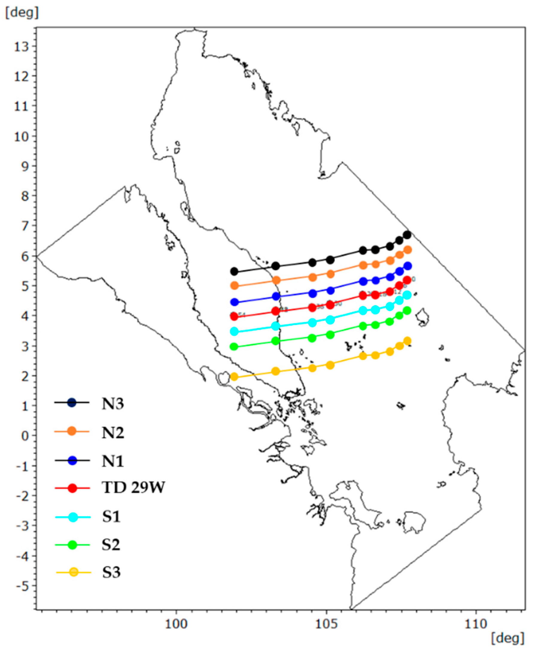
13N3NorthernMove northward, 1.5° N direction
14N2Move northward, 1.0° N direction
15N1Move northward, 0.5° N direction
16TD 29WActualDefault, 0°
17S1SouthernMove southward, 0.5° S direction
18S2Move southward, 1.0° S direction
19S3Move southward, 2.0° S direction
DSea Level Rise (SLR)
ProjectionTo examine the increase in sea level’s impact on surge variability
202040Year 2040
212060Year 2060
222100Year 2100
Disclaimer/Publisher’s Note: The statements, opinions and data contained in all publications are solely those of the individual author(s) and contributor(s) and not of MDPI and/or the editor(s). MDPI and/or the editor(s) disclaim responsibility for any injury to people or property resulting from any ideas, methods, instructions or products referred to in the content.

