Abstract
Unmanned surface vehicle (USV)-based floating-waste detection presents significant challenges. Due to the water surface’s high reflectivity, there are often light spots and reflections in images captured by USVs. Furthermore, floating waste often consists of numerous small objects that prove difficult to detect, posing a robustness challenge for object-detection networks. To address these issues, we introduce a new dataset collected by USV, FloatingWaste-I, which accounts for the effects of light in various weather conditions, including sunny, cloudy, rainy and nighttime scenarios. This dataset comprises two types of waste: bottles and cartons. We also propose the innovative floating-waste-detection network, YOLO-Float, which incorporates a low-level representation-enhancement module and an attentional-fusion module. The former boosts the network’s low-level representation capability while the latter fuses the highest- and lowest-resolution feature map to improve the model robustness. We evaluated our method by using both the public dataset FloW-img and our FloatingWaste-I dataset. The results confirm YOLO-Float’s effectiveness, with an AP of 44.2% on the FloW-img dataset, surpassing the existing YOLOR, YOLOX and YOLOv7 by 3.2%, 2.7% and 3.4%, respectively.
1. Introduction
The marine-waste problem is a global crisis that cannot be ignored and has serious negative impacts on our environment, health and economy [1]. The waste, especially plastic, causes various injuries to marine wildlife, such as entanglement, ingestion, puncture and infection. They also enter the human body through the food chain, posing a threat to human health. However, according to [2,3], waste from land-based sources is considered to be the dominant source of waste to the oceans. Thus, cleaning floating waste in inland water areas, like canals, rivers, lakes and bays, is key to reducing global marine-waste accumulation.
Manual cleaning is the dominant strategy for controlling floating waste in inland water, but it is heavy and inefficient. Furthermore, relying on manual operation is restricted by the staff’s technical abilities, and there are prospective safety risks involved when operating machines in intricate geographical areas, particularly those that operators are not familiar with. Unmanned surface vehicles as novel water platforms have shown significant potential for implementation in environmental governance due to its high efficiency, cost effectiveness and sustainability [4,5]. In particular, a real-time and accurate floating-waste-detection system is a prerequisite for the efficient and reliable autonomous cleaning of USVs. Because of the low cost of vision sensors and the wealth of information they provide, floating-waste detection relying on visual information is the most cost-effective solution. Many researchers have used vision-based floating-waste-detection methods to achieve autonomous water-surface-cleaning unmanned surface vehicles. Chang et al. [6] proposed an autonomous water-surface-cleaning unmanned surface vehicle that detects the position of waste in the image and accordingly controls the unmanned surface vehicle to collect the waste. Hasany et al. [7] proposed a robotic system for collecting floating waste that uses the object-detection results to determine whether the waste is within the robot’s collection area.
Floating-waste detection is the process of recognizing waste in the input image and determining the position of the waste in the image. With the rapid development of convolutional neural networks in object-detection tasks, a variety of networks for floating-waste detection have been proposed. Li et al. [8] proposed a novel model based on Faster R-CNN, where the Region Proposal Network (RPN) is changed from generating candidate regions to generating anchors with a reasonable aspect ratio according to the size of the object to improve the object resolution. However, it is a two-stage detector, which calculates slowly and cannot achieve real-time detection. Yang et al. [9] proposed a series of improvements based on YOLOv5 to improve the detection accuracy while maintaining the detection speed. First, a coordinate attention module is introduced in the C3 module to increase the size of the receptive field. Second, the Path Aggregation Network (PAN) is replaced by the Bidirectional Feature Pyramid Network (BiFPN) to improve the feature-extraction capability. In addition, Ouyang et al. [10] also proposed some improvements based on YOLOv5. Mixup is used for data enhancement to improve the generalization ability of the model. At the same time, the spatial-shift operation is used to improve the image-recognition accuracy. Although the average accuracy of the above models has improved compared to YOLOv5, small objects in the image still need to be noticed, especially in complex contexts. To solve the problem, we summarize the following possible reasons with floating-waste detection:
- A high proportion of small objects affects neural-network feature extraction;
- Complex surface environments have a great impact on the robustness of object-detection networks.
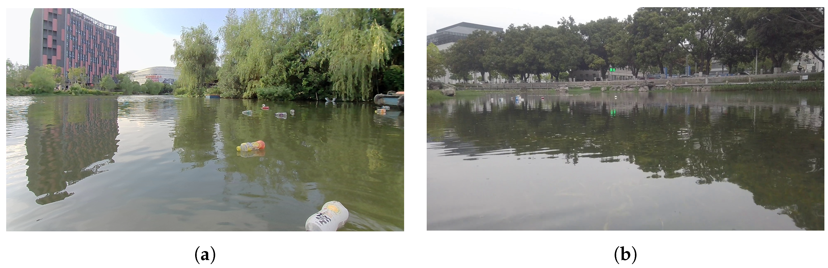
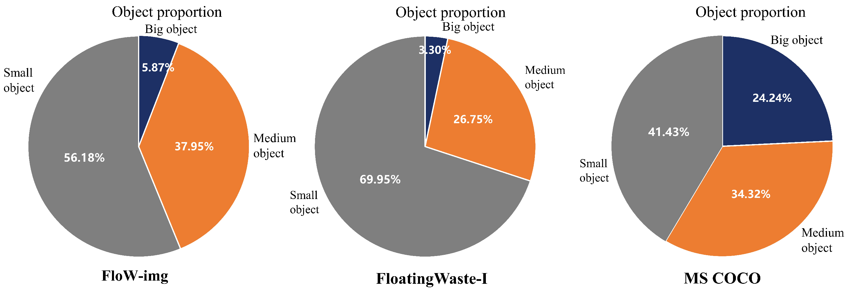
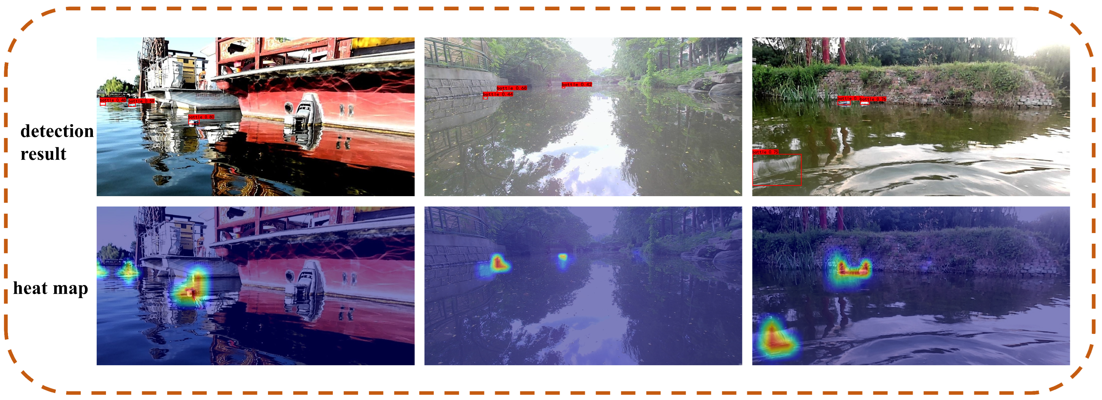
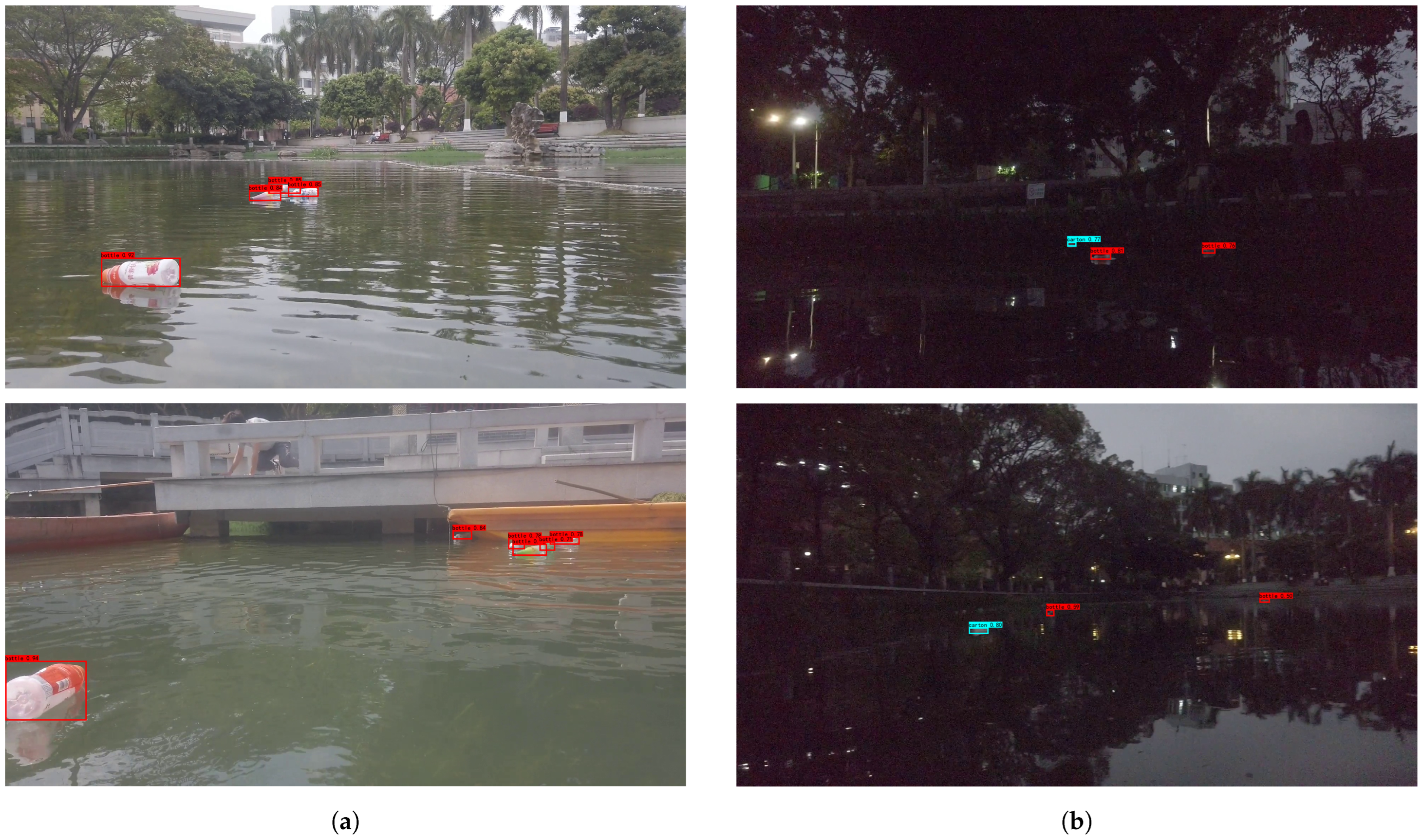
Figure 1a is an instance of the open dataset FloW-img [11], and Figure 1b is an instance of our dataset FloatingWaste-I. FloW-img and FloatingWaste-I are both collected by camera-carrying unmanned surface vehicles cruising inland waters. We can see that the bottle and carton are small compared to the large water surface. And, they are seriously interfered with by light spots, reflections and waves. We counted the proportion of large, medium and small objects in FloW-img, FloatingWaste-I and Microsoft Common Objects in Context (MS COCO) [12] according to the COCO evaluation criteria (small objects: area less than , medium objects: area greater than and less than , large objects: area greater than ). It shows that the proportion of small objects in FloW-img and FloatingWaste-I is higher than MS COCO. From the Figure 2, we can see that the proportion of small objects in FloW-img and FloatingWaste-I account for 56.18% and 69.95%, respectively, which is much higher than the 41.43% in MS COCO. It indicates that the high proportion of small objects is a common problem of floating-waste datasets, as shown in Figure 3. The detection results and the heat map show that the light spots formed by sunlight and the reflections formed by the surrounding environment are easily misidentified as objects. It indicates that the floating-waste detection is strongly interfered with by the complex background on the water surface.

Figure 1.
The floating-waste dataset. (a) An image from FloW-img dataset. (b) An image from FloatingWaste-I dataset.

Figure 2.
Percentage of large, medium and small objects in the FloW-img dataset, FloatingWaste-I dataset and MS COCO dataset.

Figure 3.
YOLOv5 detection results on FloW-img with a heat map, with similar features of light spots and reflections being mistaken for objects.
In recent years, YOLOv5 has been widely used in many scenarios in the field of real-time object detection, such as face recognition [13,14], autonomous driving [15,16] and agricultural robots [17,18]. It is fast, accurate, easy to configure and easy to set up. Although YOLOv5 performs well in many scenarios, due to the large proportion of small objects and strong background interference in the floating-waste dataset, a large number of false detections and missed detections occur in the detection results when YOLOv5 is applied directly. Based on the above phenomenon, we summarize the following three possible reasons: (1) Features of small objects are easily lost when downsampling in the backbone. (2) The high-resolution feature map contains a lot of similar redundant information. (3) The highest-resolution and lowest-resolution feature map are not sufficiently integrated. To address the above problems, we propose a novel real-time floating-waste-detection model called YOLO-Float. The main contributions of our research are as follows:
- We design a low-level representation-enhancement module, which consists of a multiscale convolution part and a region-detection head. The designed module enhances the low-level representation capability of the feature maps, effectively solving the problem that features of small objects are easily lost when downsampling in the backbone.
- We propose a new feature-fusion module to fuse the highest-resolution and lowest-resolution feature maps. The proposed module effectively fuses features by learning the correlations between feature maps at different levels, which reduces the transfer of redundant information.
- We construct a new floating-waste dataset called FloatingWaste-I (detailed in Section 4.1). The proposed dataset has more floating-waste categories (carton and bottle) and more light conditions (cloudy, rainy, sunny and evenfall). And, YOLO-Float is compared with current state-of-the-art models on the public FloW-img and FloatingWaste-I datasets to verify its effectiveness.
The rest of this paper is organized as follows. In the Section 2, we review some of the relevant research involved to facilitate understanding of our work. In the Section 3, we elaborate our problem-solving ideas and methods based on the relevant work and theory mentioned above. In the Section 4, we conduct experiments by using the proposed method on both the FloW-img and FloatingWaste-I datasets to verify its effectiveness and progressiveness. In the Section 5, we provide a systematic summary of the entire work and an outlook for future work.
2. Related Work
2.1. Water-Surface-Object Dataset
Benefiting from the rapid development of the unmanned field, research on unmanned surface vehicles has received increasing attention, and many datasets have emerged in the field of surface-object detection, effectively supporting the development of surface-object detection. In order to simulate the hazards that USVs may encounter while navigating realistically, researchers proposed the Marine Obstacle-Detection Dataset (MODD) [19] and the Multimodal Marine Obstacle-Detection Dataset (MODD2) [20], which were collected by manually operating an unmanned vessel. They both contain multiple weather conditions (sunny, cloudy and foggy) and various extreme conditions (vigorous motion and sunlight reflection). The Singapore Marine Dataset (SMD) [21] was collected in Singapore waters by D.K. Prasad et al. It was collected by using shore-based fixed-platform cameras and shipboard cameras. The dataset contains 10 different types of objects, including ships, ferries, speedboats and sailboats, which were collected at six different times of day and in different environments, such as rain and fog. However, the above marine-object dataset differs significantly from the inland floating-waste dataset and cannot be used as an experimental benchmark. There are two major areas:
- The sea has a less distracting background than inland waterways, with mainly light patches and ripples, and a lack of reflections from trees, houses and roads;
- Large objects such as ships and ferries make up a great part of the marine dataset.
The FloW-img dataset is the first inland floating-waste dataset collected by USVs with a camera on board. When collecting the dataset, the variety of collection scenes, lighting conditions, number of objects per frame, appearance of the objects, view angles and target ranges are considered to increase the diversity of the samples. The image dataset contains 2000 images with 5271 labeled pieces of floating waste. Additionally, it also provides 200 video sequences without annotations in the FloW-img dataset, which can be used to support studies on floating-waste tracking. This benchmark has greatly facilitated the work of USVs in detecting floating objects on the water. But, the dataset only contains one class of detection object, so we construct a new floating-waste dataset.
2.2. Object Detection
Most traditional detection algorithms are based on a sliding-window approach, where the image is traversed by setting different window sizes to extract manually designed features, followed by template matching and feature learning to detect potential objects [22,23,24]. In 2014, Girshick et al. pioneered the convolutional neural network (R-CNN) [25], which led to the rapid development of deep-learning-based object-detection methods. At present, deep-learning-based object detection can be mainly divided into two streams: the two-stage detectors [26,27,28] and the one-stage detectors [29,30,31] pioneered by YOLO. In general, two-stage methods tend to be more accurate than one-stage methods because they use RPN to balance positive and negative samples. However, the performance gap between the two has disappeared recently. The YOLOv5 [32] is the first widely used one-stage detector that outperforms two-stage detectors. In this paper, we implemented YOLO-Float based on YOLOV5.
3. Proposed Method
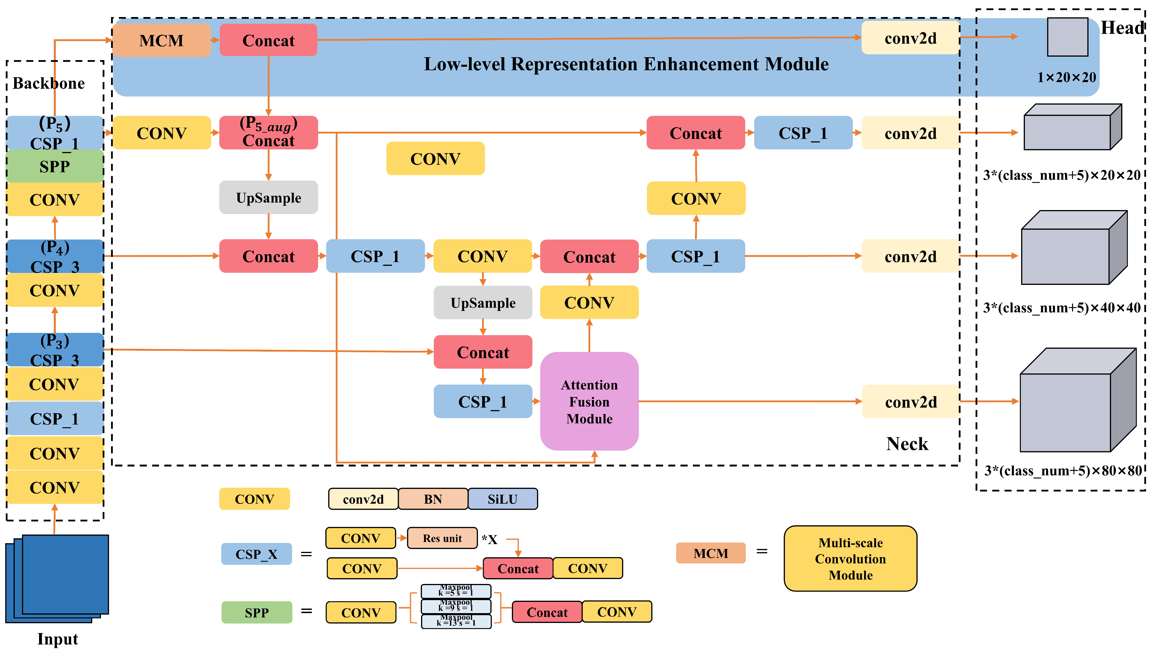
The structure of YOLO-Float is shown in Figure 4. YOLO-Float mainly consists of a backbone, neck and head. For this method, after feeding the data-enhanced image into the network, features are first extracted through the backbone. Further feature extraction and fusion is conducted by four branches in the neck. Finally, three heads predict the main task and one head predicts the branch task. The backbone of YOLO-Float is consistent with YOLOv5, using three main structures CONV, CSP and SPP, which can reduce the amount of repeated gradient information during backpropagation to reduce computation. In the neck and head part, we propose the low-level representation-enhancement module (LREM), which uses a multiscale convolution module to extract feature information with different receptive field sizes to predict the object region. In the neck part, we propose the attention-fusion module (AFM) to fuse the and feature maps, and the details of each module are described below.

Figure 4.
The YOLO-Float framework. The network consists of three parts: backbone, neck and head. In the backbone, the block consisting of CONV, CSP and SPP is used to extract the features (the composition of CONV, CSP and SPP is shown in the figure). After that, the low-level representation-enhancement module is used to ensure that features of small objects are not lost when downsampling in the backbone. Meanwhile, the attention-fusion module is used to fuse highest-resolution and lowest-resolution feature maps. Finally, the head predicts the results of the region classification. And, the other three heads predict the results of the classification and bounding-box regression. Since each grid on the feature map is preset with three anchors of different aspect ratios, for each anchor, it predicts the horizontal and vertical coordinates of its center point, width, height, confidence level and the class to which it belongs, so the number of feature channels for the three heads is .
3.1. Low-Level Representation-Enhancement Module
In YOLOv5, the input image generates (), () and () feature maps after the convolutional neural network downsampling operation in the backbone. However, due to the small size of the objects in the floating-waste dataset, the resolution of the positive samples distributed on the , and feature maps is too low. This causes the features that highlight the objects to be lost in the downsampling operation of the backbone. Considering the coherence and density of the backbone and neck structure in YOLOv5, the low-resolution feature maps can capture the rough location information of the objects, even if many details of the objects are lost. Therefore, we propose a module to judge whether objects exist in each region of the low-resolution feature map. This module ensures that the object’s features are not lost during the downsampling process by constraining the low-resolution feature map to learn the object’s location information. Since the details of the objects in the low-resolution feature map may be too tiny to enhance the high-level representations well, its main effect is to indirectly enhance the low-level representation of high-resolution feature maps, so we call it the low-level representation-enhancement module.
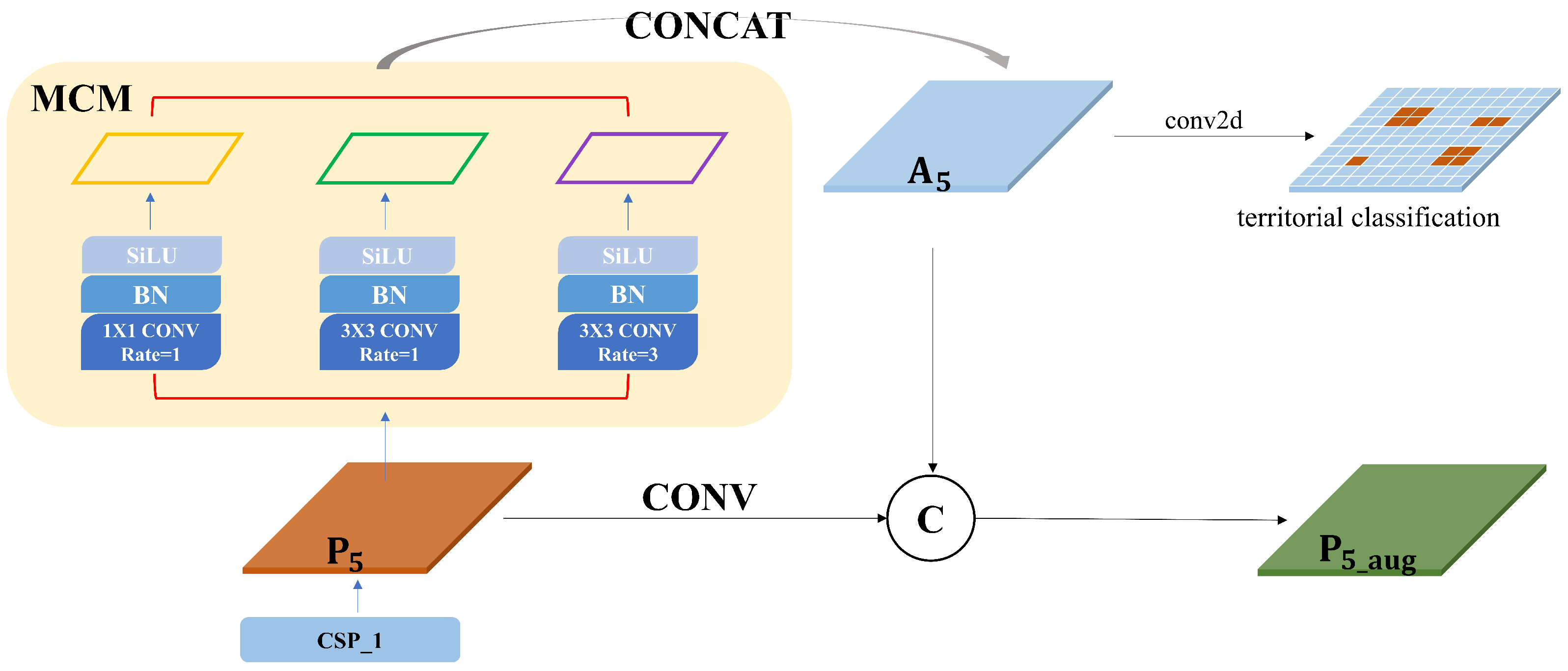
The low-level representation-enhancement module is shown in Figure 5, and we introduced the module on the feature map after the last CSP_1 structure of the backbone. A single-scale convolutional procession results in a narrow receptive field. It is not sufficient to cover all objects while the objects vary greatly in size. Thus, we used a multiscale convolutional module (MCM) consisting of the dilated convolution. Dilated convolution is the process of injecting holes into the standard convolution map in order to increase the receptive field. The dilation rate refers to the number of intervals between each point in the kernel. In total, we use a dilated convolution kernel of size with a dilation rate of 1, a dilated convolutional kernel of size with a dilation rate of 1 and a dilated convolution of size with a dilation rate of 3 to convolve . Following batch normalization and the activation function, the feature maps with different receptive field sizes are obtained. After concatenating them together, the feature map is obtained. Then, the feature map is convolved to obtain the territorial classification for prediction where the brown areas indicate the presence of objects and the light blue areas indicate the absence of objects. It is also concatenated with to obtain the enhanced feature map . Specifically, the territorial classification map is to predict whether the region mapped to the original images contains the object. In other words, it learns the location information of the floating-waste object. Only the grid cells containing the center of the object are taken as positive samples, and the rest of the grid cells are not involved in the training. Grid cells containing the background region are taken as negative samples.

Figure 5.
Low-level representation-enhancement module. Note that the symbol C represents the concatenation that links the channels of two feature maps of the same size. BN represents the batch normalization, which has the effect of preventing overfitting and accelerating convergence. SiLU represents the nonlinear activation function Sigmoid Linear Unit, , where is the logistic sigmoid.
3.2. Attention Fusion Module
As the number of layers of the network increases, the receptive field of the network becomes progressively larger and the semantic expressiveness increases. However, this also reduces the resolution of the image, and many detailed features become increasingly blurred after the convolution operation. This means that the high-resolution feature maps have a small receptive field and a strong expression of the detailed features to detect small objects well. The low-resolution feature maps are better at accurately detecting objects as the semantic information. Multiscale feature fusion [33,34] can synthesize information from different scales to extract richer and more diverse features, improving the performance and robustness of computer vision tasks. YOLOv5 uses PAN to shorten the information path between lower layers and the topmost feature by bottom-up path augmentation. However, it is not an effective method because it results in the loss of the semantic information in the lowest-resolution feature map. In addition, the feature map contains richer information after the LREM, and we cannot guarantee that the effectiveness of the information is maintained through successive upsampling operations. This requires the effective fusion of the lowest- and highest-resolution feature maps.
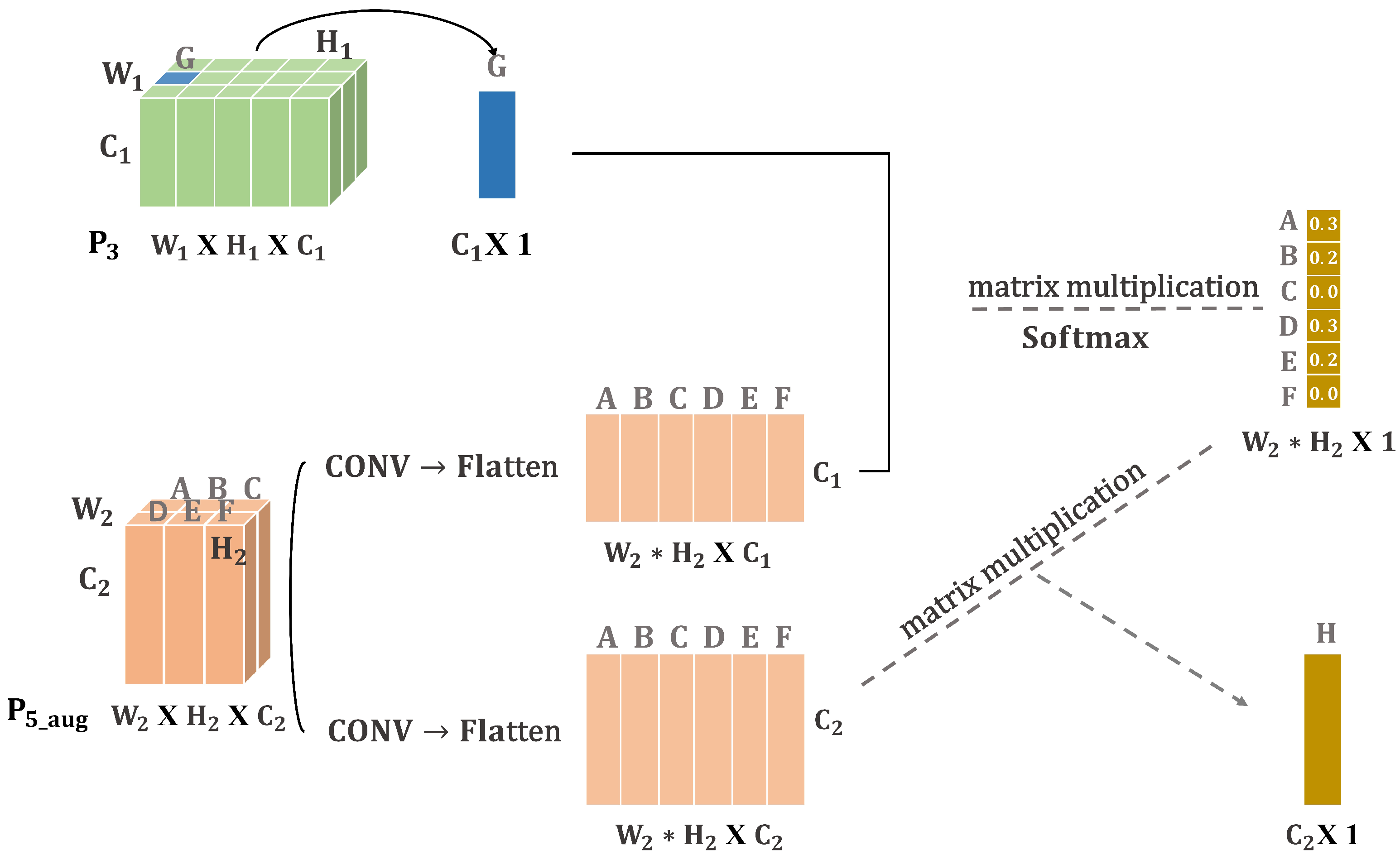
The lowest-resolution feature map and the highest-resolution feature map are very different in size and dimension, and it is difficult to align the same feature on these two feature maps. The self-attention mechanism at the core of the transformer [35,36] captures correlations between its own internals. Therefore, to effectively fuse feature maps across hierarchies, we could fuse the two feature maps based on their correlation. As shown in Figure 6, we want to find which features in the feature map are of interest to the G feature. So, we first reduce and flatten the feature map. Then, we normalize it by multiplying it with the G feature. This gives us the attention value of the G feature for each feature in the feature map. We can see that the G feature has a high correlation with the A, B, D and E features. Finally, we multiply the feature map by the attention matrix to obtain the feature H that has the highest correlation with feature G. This approach can effectively fuse the lowest-resolution and highest-resolution feature maps, although their hierarchies are very different. It better filters the background and improves the robustness of the whole network. Then, we will explain the attention-fusion module in detail.

Figure 6.
Example of attention-fusion module. Note that the G represents the feature of the feature map. The A, B, C, D, E, F represent the feature of the feature map. Broadcasting the G feature to the whole feature map is the process of fusion of the two feature maps.
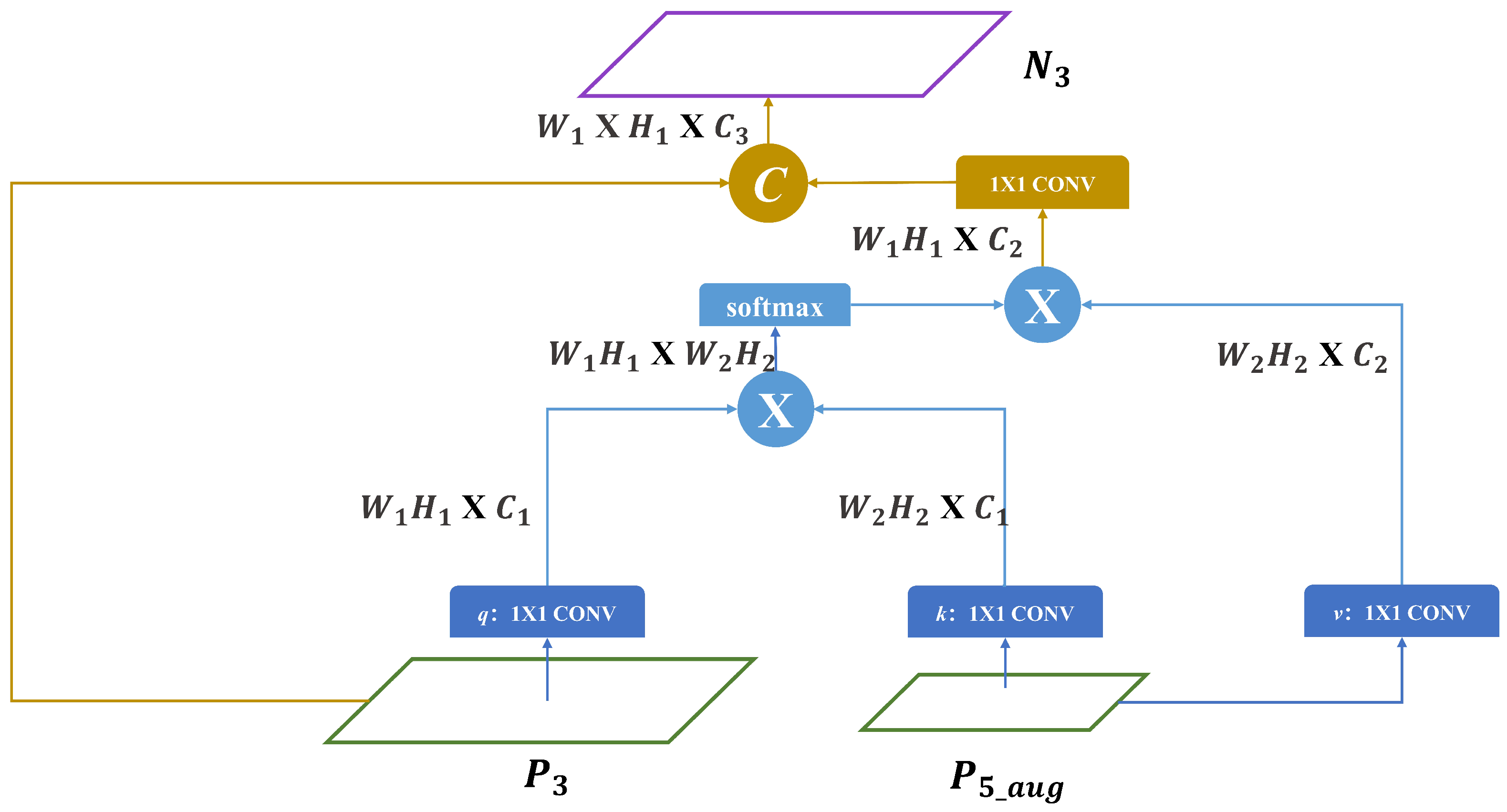
As shown in Figure 7, referring to the transformer, the attention-fusion module can be expressed as Equation (1). The attention-fusion module has two inputs ( and ) and one output , which we define as , and , respectively. denotes the magnitude of the tensor:

Figure 7.
Attention-fusion module. We still follow the terminology of three different vectors in transformer. q: query vector. k: vector representing the relevance of the queried information to other information. v: vector representing the queried information. The output of each row results in the shape of a tensor, where denotes the product of and . The symbol “×” denotes matrix multiplication and the symbol “C” denotes the concatenation.
We use a convolution kernel of size to downsample and . So, they have the same number of channels. And, we flatten them to change the dimension of the tensors to obtain q and k. Then, matrix multiplication is used to obtain the relationship matrix , as shown in Equation (2):
The above function acts to change the tensor dimension. As shown in Equation (3), is the output of the . It can be represented by the vector . can be represented by the vector . The dimensions of the vectors x,y are both , so the relation matrix can be expressed as Equation (4):
The relationship matrix is normalized by using Softmax to obtain the weight coefficients, which can be expressed as Equation (5):
Then, we use a convolution kernel of size to downsample and flatten it to obtain v. We multiply v by the weight coefficients to obtain the feature map with the strongest correlation with . Finally, we convolve this feature map and concatenate it with to obtain the fused feature map .
3.3. Loss Functions
YOLO-Float contains three subtasks: region classification, object-detection classification and object-detection localization, corresponding to three loss functions: two classification loss functions and a box-regression loss function, as shown in the following Equation (6):
We use the stochastic gradient descent method to jointly train the three subtasks. For classification loss, considering the prevalence of the background interference in negative samples, we use the cross-entropy loss function as the two classification loss functions, as shown in the following Equation (7).
where y is the ground truth and is the predicted value. The box-regression loss provides an important learning signal to accurately locate the anchor box. Because the small objects occupy the main part, it is easy for the ground truth to not overlap with the anchor box. We use GIoU loss [37] to address the problem of a loss equal to 0 when the ground truth does not overlap with the anchor box, as shown in the following Equation (8):
where the is the intersection over union. A is the prediction box, B is the ground truth and C is the boundary that surrounds A and B with a minimum rectangle.
4. Experiments
This section first introduces the FloW-img and FloatingWaste-I datasets. Then, the role and effectiveness of each module are analyzed. Finally, YOLO-Float is compared with current state-of-the-art object-detection algorithms on the FloW-img and FloatingWaste-I datasets.
4.1. Dataset and Implementation Details
4.1.1. FloW-Img Dataset
As shown in Table 1, the FloW-img dataset is the world’s first open-water floating-waste-detection-image dataset in a real inland waterway scenario and from the perspective of an unmanned surface vehicle. The dataset was obtained by using an unmanned surface vehicle with two cameras cruising an inland river. The lighting conditions of the scenes are all daytime and the diversity of the scenes is high. A total of 2000 images were obtained by sampling the video sequences. The image resolution is and . The data are labeled as “bottle”. The number of samples is 5272, and the reflection of the bottle is excluded from the label area to avoid ambiguity when labeling the data.

Table 1.
Comparison of public datasets on water-surface object detection in the number of annotated frames, type of detection object, number of object classes, resolution of image, type of environment, view of USV and condition of light. Environment: M—marine, I—inland. USV-based: Y—yes, N—no. Condition: L—light, D—dark.
4.1.2. FloatingWaste-I Dataset
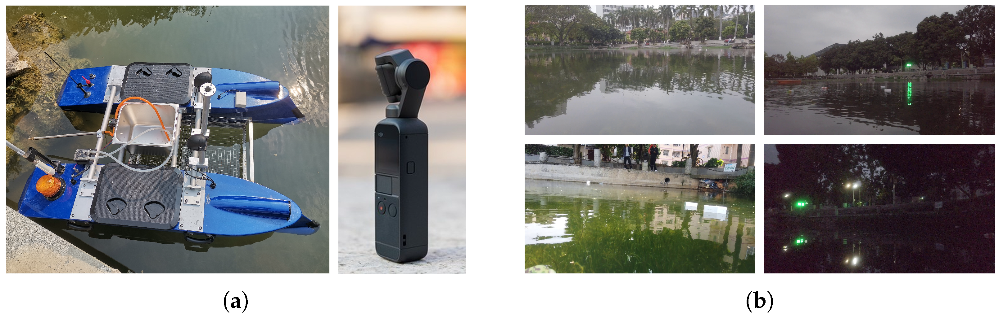
The FloatingWaste-I dataset is a multicategory floating-waste dataset containing bottles and cartons, which are two common types of domestic waste found on water. During the data-collection phase, we used an unmanned surface vehicle equipped with a DJI Pocket2 motion camera to cruise around the four lakes on the campus of Guangxi University. The FloatingWaste-I dataset was acquired in three time periods: midday, evening and night. As shown in Figure 8, the unmanned surface vehicle used in this paper mainly consists of a hull-power module, wireless control and other modules. After installing the DJI Pocket2 motion camera, we controlled the unmanned surface vehicle to cruise the lake to photograph floating waste. In the data-annotation phase, we used labeling to annotate the data. To create the labels, we used rectangular boxes to completely cover the objects, labeled, respectively, “carton” and “bottle”. In line with FloW-img, we do not mark the object reflection inside the label area.

Figure 8.
Acquisition platform and environment. (a) The unmanned surface vehicle and DJI Pocket2 motion camera. (b) The scenario and time of collection phase.
In addition, to ensure the quality of the labels, our team of three people strictly implemented the labeling procedure to manually label the data and screened out the controversial labels to vote on whether the labeling was qualified or not. In the end, we collated 1867 images with a resolution of , including 3213 samples of bottles and 1302 samples of boxes.
4.1.3. Evaluation Metrics
In this paper, precision and recall are used as metrics to validate the model accuracy. Precision is the ratio of the number of detected positive samples to the total number of detected samples, i.e., TP/(TP + FP), where TP is true positive and FP is false positive. The recall is the ratio of the number of detected positive samples to the total number of positive samples, i.e., TP/(TP + FN), where FN is false negative.
To describe the effect presented by the model in this paper, we use (the mean average precision) and (the mean average recall) [38] to evaluate the accuracy of the model. calculates the area under the PR curve for a given category, while calculates the average of the areas under the PR curve for all categories. is the average of all IoU recalls on [0.5,1.0]. It is twice the area enclosed by the recall-IoU curve. is the average of for all categories. The formula is as follows:
where P, R and N represent precision, recall and the total number of instances in all categories, respectively. For , we also used the five metrics including , , , and , which measure the overall average-accuracy rate, the overall-positioning average-accuracy rate, the small-object average-accuracy rate, the medium-object average-accuracy rate and the large-object average-accuracy rate, respectively. For , we also used the five metrics including , , and , which measure the overall average recall rate, the small-object average-recall rate, the medium-object average-recall rate and the large-object average-recall rate, respectively.
4.1.4. Experimental Platform and Parameters
To ensure the fairness of the experiments, all the experiments in this paper were conducted under the Pytorch framework with the hardware facilities of CPU: Intel(R) Xeon(R) Gold 6136 CPU @ 3.00 GHz, graphics card: GeForce GTX TITAN X and memory: 12 GB, and all the models were trained by using the SGD optimizer for 300 epochs. The batch size was set to eight and the initial learning rate was set to 0.01 by using the learning-rate-decay method.
4.2. Results of the Experiments
4.2.1. Ablation Studies
In order to verify the validity of YOLO-Float and to fully investigate the validity of the individual modules of the proposed algorithm, we set up ablation experiments as (a) YOLOv5, (b) YOLOv5 with LREM, (c) YOLOv5 with AFM and (d) YOLOv5 with all the modules Float.
Table 2 shows the experimental results of the four models, where we conducted ablation experiments on FloW-img and analyzed the effectiveness of each module. and denote the threshold of an IOU of 0.5:0.95 and 0.75, respectively. represents the average accuracy, and better highlights the localization average accuracy. , and denote the average accuracy of the small, medium and large objects, respectively. , and indicate the average recall for the small, medium and large objects, respectively. Comparing the YOLOv5 and YOLOv5 + LREM models, the addition of the LREM improves by 5%, by 1.5% and by 1%. The LREM effectively improves the object-localization ability and small-object-detection ability of the model. Comparing the YOLOv5 and YOLOv5 + AFM models, the addition of the AFM improves the overall average accuracy by 2%, with improving by 2.5%, improving by 2.8%, improving by 2.8% and improving by 2.7%. The AFM effectively improves the accuracy and recall of the large and small objects. It shows that the lowest-resolution and highest-resolution feature maps fused by the attention-fusion module not only help the shallow feature map to better predict small objects but also help the deep-feature map to better predict the large objects. Comparing the YOLOv5 with the YOLO-Float model, adding both the LREM and AFM improved the average accuracy by 2.4%, by 6.7%, by 4% and by 3.7%. The YOLO-Float model performs best among the four groups of experiments. Through the above comparison, we found that each of the modules proposed in YOLO-Float helps to improve the detection accuracy of the model.
Table 2.
Ablation experiments on FloW-img.
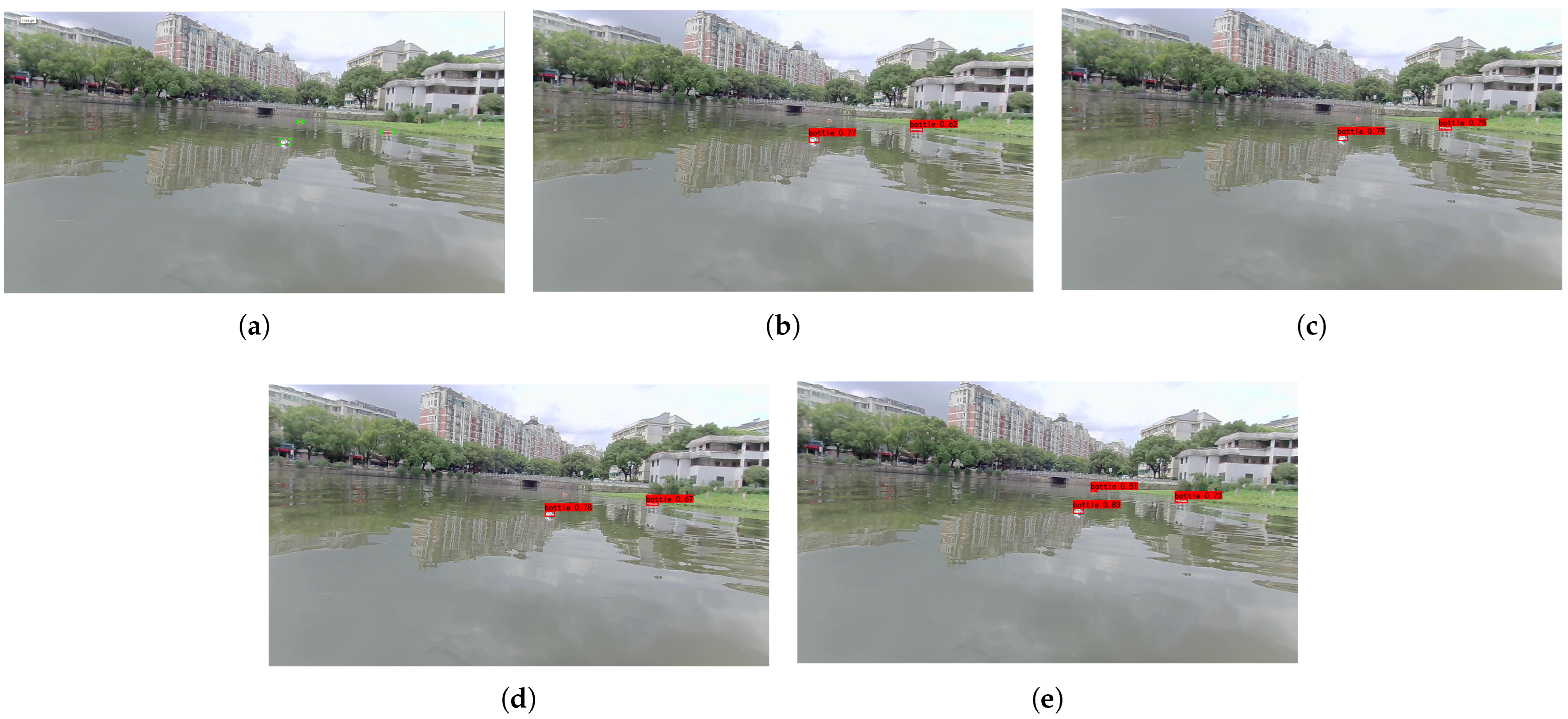
In order to show the effect of each module more visually, we chose a random image to show the detection results of the four models. As shown in Figure 9, comparing Figure 9d with Figure 9b and Figure 9c with Figure 9b, we can find that the detection of objects is more accurate after adding the LREM and AFM. It indicates that the LREM and AFM can enhance the robustness of the network. Comparing Figure 9e and Figure 9b, we can find that our algorithm YOLO-Float can accurately identify smaller objects in the distance. It shows that the detection capability of the network for small objects is significantly improved.

Figure 9.
Detection results of different models. (a) Ground truth, (b) YOLOv5, (c) YOLOv5 + LREM, (d) YOLOv5 + AFM, (e) YOLO-Float.
4.2.2. Effectiveness of Loss Curve
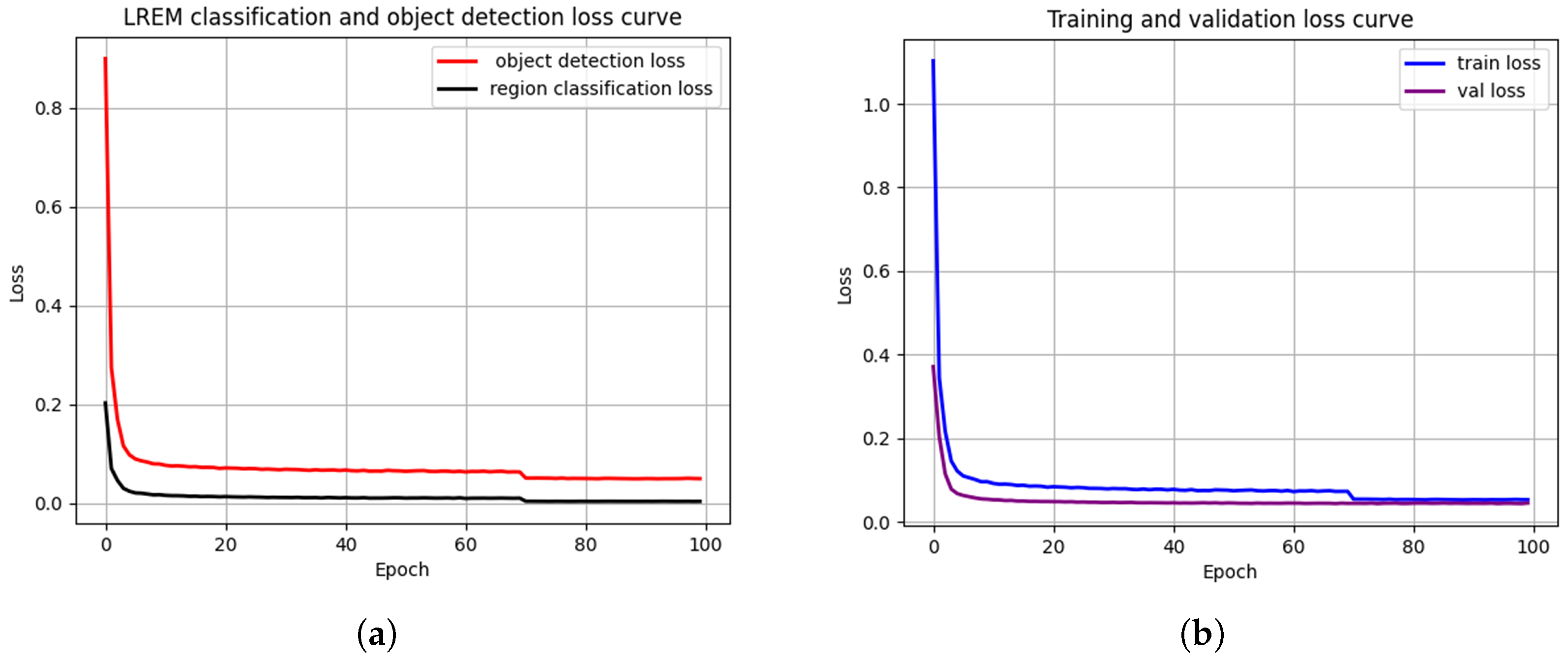
To further illustrate the effectiveness of the LREM, as shown in Figure 10, we analyzed the trend of the decreasing loss in the object detection and LREM classification during the training phase of the model YOLOv5 + LREM. The loss curve reflects the change in the value of the loss function with the number of training steps. During the training process, we can observe the loss curve to determine whether the model converges or not. We can also observe the object-detection and LREM-classification loss curves to judge the effectiveness of the LREM. For example, when the loss curve of the object detection shows a decreasing trend and the loss curve of the LREM classification shows an increasing trend, the LREM is disadvantageous to the object detection.

Figure 10.
The loss curves of the model YOLOv5 + LREM in the training phase. (a) LREM-classification loss curve and object-detection loss curve, which can be seen to have a similar decreasing trend. (b) Training loss curve and validation loss curve.
The experiment set up 100 epochs to train the LREM classification and the object detection. As shown in Figure 10, during the training process, the loss declines rapidly and enters the slow-decline phase after five epochs. In the slow decreasing phase, the LREM classification loss and the object-detection loss converge and show a steady decrease with several fluctuations. It shows that they have a strong relationship.
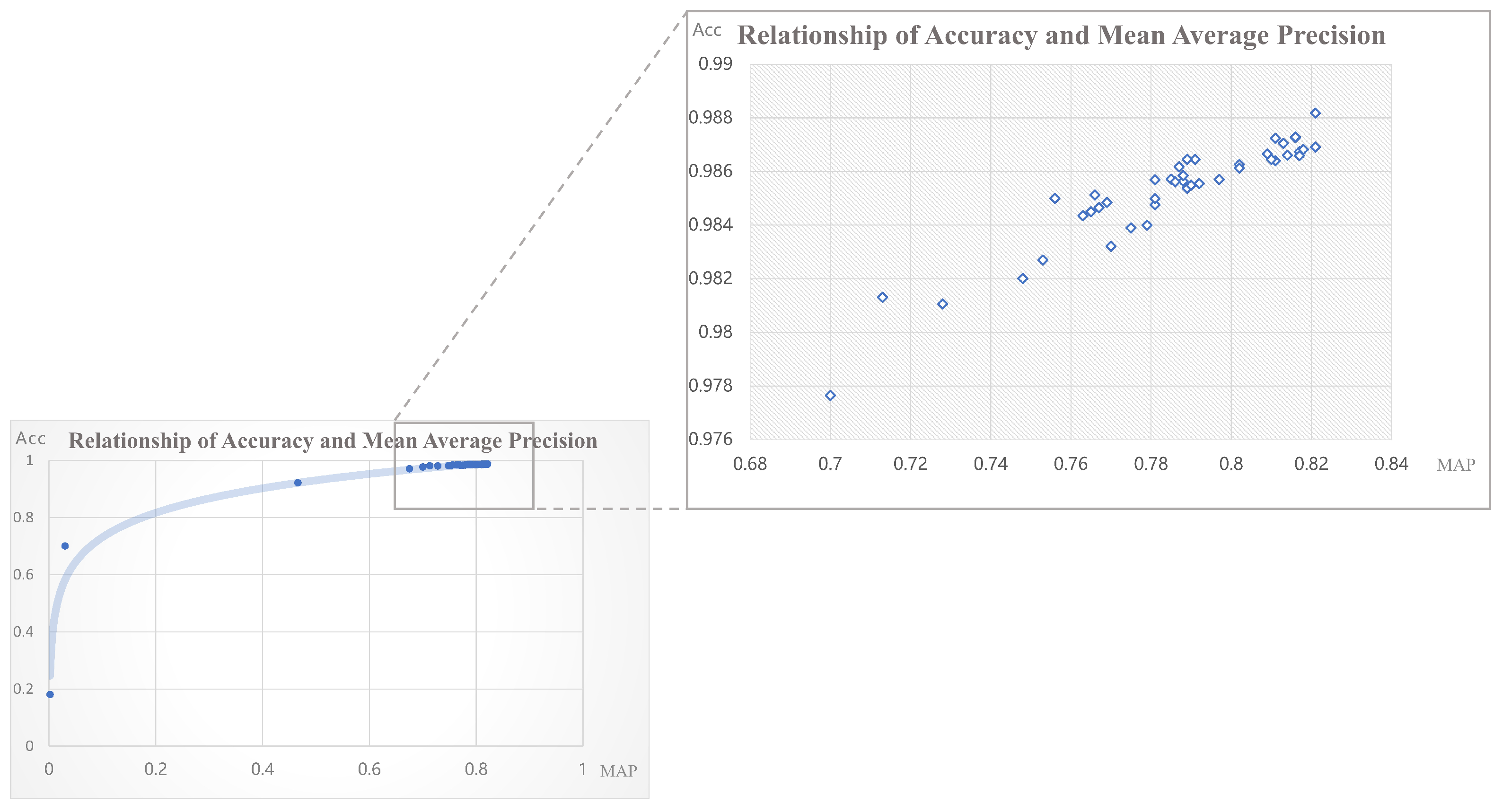
In order to further demonstrate the relevance of the objection detection and LREM classification, as shown in Figure 11, we count the region-prediction results and the object-detection results for each epoch corresponding to the weights in the training phase. And, we plot the LREM classification accuracy as the X-value and the object-detection as the Y-value in the scatter plot. It can be seen that the LREM classification accuracy improves faster than the object-detection at the early stage of training, and the two are positively related. When the improvement stabilizes, they still have a strong positive relationship within a small range of accuracy changes, proving that the LREM is beneficial for object detection.

Figure 11.
Scatterplot of LREM-region classification accuracy and object-detection mAP in the training phase. The points in the scatter plot correspond to the LREM-classification metric accuracy and object-detection metric MAP under the weights obtained from the epochs in the training phase.
4.2.3. Effectiveness of AFM
To further illustrate the effectiveness of the AFM, we set up experiments to compare and analyze the direct upsample with the attentional-fusion module. Upsample refers to the enhancement of the feature-map resolution by interpolation. Using the upsampling fusion-feature map, as shown in Figure 7, only is upsampled by a factor of four and then concatenated with . The experimental results are shown in Table 3. It can be seen that both methods improved in all aspects compared to YOLOv5, especially in object localization and small-object prediction. The upsampling fusion method increased the by 3.8%, by 1.8% and by 1.7% compared to YOLOv5. It indicates the importance of fusing the and feature maps. The AFM still shows an improvement of nearly 0.8% in each metric compared to the upsampling fusion method, which shows that the AFM is more reasonable and effective than the upsampling method. Our analysis suggests that interpolation introduces a lot of noise and blurs the feature map. Simply enlarging the feature map by a factor of four also does not accurately align the feature map. However, the AFM focuses on the correlation between two feature-level grid cells. It matches them by the similarity of their own features. This is able to better fuse the lowest-resolution and highest-resolution feature maps, making the fusion a much better performer.
Table 3.
Ablation experiments on FloW-img.
4.3. Comparison with Other Methods
4.3.1. Object Detection on FloW-Img
We compare YOLO-Float with the YOLO series of advanced algorithms and other two-stage detectors on the FloW-img dataset, and the quantitative experimental results are shown in Table 4. We set the version of each model according to [39] and put the benchmark [11] of FloW-img at the bottom of the table. We still use the COCO evaluation metric, focusing on the algorithm’s small-object-detection effectiveness and localization capability. It can be seen that the , and of YOLO-Float are the best among the compared methods, reaching 44.2%, 42% and 30.7%, respectively. The excellence of our algorithm is not only in the improvement in the overall average accuracy but also in the improvement in the localization ability and small-object detection.
Table 4.
Comparison experiment on FloW-img.
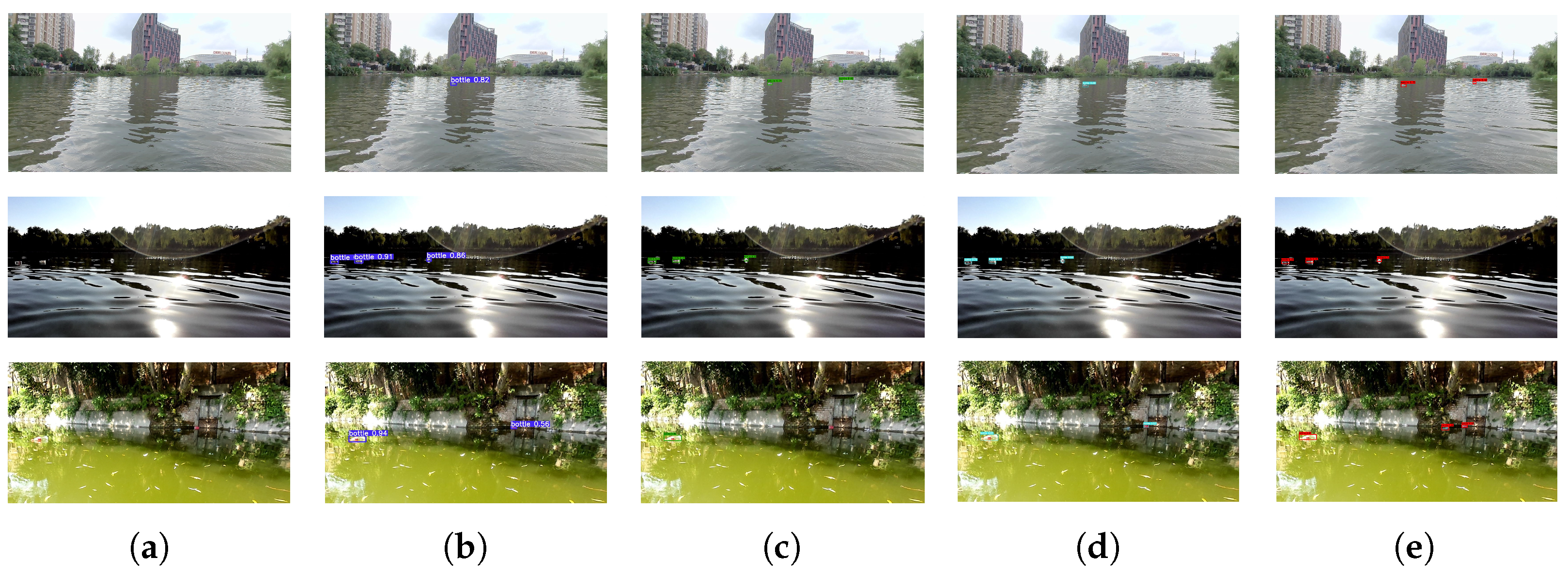
To show our algorithm more intuitively, Figure 12 gives the object-detection results of different algorithms in three typical scenarios in FloW-img. Scene one shows floating waste far away and a small object size. Scene two shows strong light interference. Scene three shows high light variation and strong background interference. It can be seen that YOLO-Float can correctly predict most objects with high confidence compared to other algorithms.

Figure 12.
Detection results of different algorithms. (a) The input image, (b) the result of YOLOR, (c) the result of YOLOX, (d) the result of YOLOv7, (e) the result of proposed method.
4.3.2. Object Detection on FloatingWaste-I
We compare YOLO-Float with the YOLO-series of advanced algorithms on the FloatingWaste-I dataset, and the quantitative experimental results are shown in Table 5. It can be seen that the , and of YOLO-Float are still the best among the compared methods, reaching 37.8%, 30.4% and 23.6%, respectively. YOLO-Float shows better stability and efficiency. In the presence of multiple object categories, as shown in Table 6, YOLO-Float is able to learn the geometric features of the different categories of objects well and accurately detect the objects in each category. In addition, as shown in Figure 13, YOLO-Float is still able to detect the object accurately, even if the object is obscured and not complete. The attention-fusion module of YOLO-Float is able to effectively extract the rich information of the semantic context to help the network identify the defective geometric features. YOLO-Float can still detect the object well when the light is low, the reflections from the water surface are strong and the geometric features are not obvious. Thanks to the LREM and AFM, the network has an excellent feature-extraction capability and anti-interference ability.
Table 5.
Comparison experiment on FloatingWaste-I.
Table 6.
Comparison experiment on FloatingWaste-I with different class.

Figure 13.
Detection results of YOLO-Float on FloatingWaste-I. (a) represents the object occlusion, (b) represents the evening scene.
5. Discussion and Conclusions
At this stage, with the rapid development of object-detection tasks, many researchers have applied networks for the detection of floating waste to solve the problem of marine pollution. Based on previous research, we propose the YOLO-Float detection network, which contains a low-level representation-enhancement module and an attention-fusion module, to address the characteristics of small targets and high background interference on the water surface. The low-level representation-enhancement module predicts the region where the object is located on the lowest-resolution feature map. It uses the dilated convolution to widen the receptive field range and enhance the low-level representation of the network. The attention-fusion module fuses the lowest-resolution and highest-resolution feature maps through the attention mechanism. Experimental results show that the YOLO-Float network performs well on the FloW-img dataset and the FloatingWaste-I dataset. It better meets the accuracy and robustness requirements for the detection of floating waste on the water surface.
Our method focuses on the improvement in the detection accuracy and not the detection speed. The lightweight improvement in the network is our future research direction. In addition, the collection scene of the FloatingWaste-I dataset is relatively single compared to FloW-img. The expansion of the FloatingWaste-I dataset is also our future research focus.
Author Contributions
Conceptualization, Y.L.; methodology, R.W., D.G. and Y.L.; software, R.W.; validation, R.W. and Z.L.; writing—original draft preparation, R.W. and Y.L.; writing—review and editing, R.W., Y.L. and D.G.; supervision D.G.; project administration, Y.L. and D.G. All authors have read and agreed to the published version of the manuscript.
Funding
This research was funded by the Guangxi Science and Technology base and Tlalent Project (Grant No. Guike AD22080043), the Key Laboratories of Sensing and Application of Intelligent Optoelectronic System in Sichuan Provincial Universities (Grant No. ZNGD2206) and Guangxi Science and Technology Program: Guangxi key research and development program (Grant No. Guike AB21220039). Key Laboratcry of AI and Information Processing (Hechi University), Education Department of Guangxi Zhuang Autonomous Region (Grant No. 2022GXZDSY006). The APC was funded by Yong Li.
Institutional Review Board Statement
Not applicable.
Informed Consent Statement
Not applicable.
Data Availability Statement
COCO dataset: https://cocodataset.org/#download (accessed on 10 October 2023); FLOW dataset: https://orca-tech.cn/datasets/FloW/Introduction (accessed on 10 October 2023). FloatingWaste-I dataset: https://github.com/wangruichen01/FloatingWaste-I (accessed on 10 October 2023).
Acknowledgments
The authors thank the Guangxi Key Laboratory of the Intelligent Control and Maintenance of Power Equipment for the device support.
Conflicts of Interest
The authors declare no conflict of interest.
References
- Li, W.C.; Tse, H.F.; Fok, L. Plastic waste in the marine environment: A review of sources, occurrence and effects. Sci. Total Environ. 2016, 566, 333–349. [Google Scholar] [CrossRef]
- Jambeck, J.R.; Geyer, R.; Wilcox, C.; Siegler, T.R.; Perryman, M.; Andrady, A.; Narayan, R.; Law, K.L. Plastic waste inputs from land into the ocean. Science 2015, 347, 768–771. [Google Scholar] [CrossRef] [PubMed]
- Lebreton, L.; Van Der Zwet, J.; Damsteeg, J.W.; Slat, B.; Andrady, A.; Reisser, J. River plastic emissions to the world’s oceans. Nat. Commun. 2017, 8, 1–10. [Google Scholar] [CrossRef]
- Akib, A.; Tasnim, F.; Biswas, D.; Hashem, M.B.; Rahman, K.; Bhattacharjee, A.; Fattah, S.A. Unmanned floating waste collecting robot. In Proceedings of the TENCON 2019—2019 IEEE Region 10 Conference (TENCON), Kochi, India, 17–20 October 2019; pp. 2645–2650. [Google Scholar]
- Ruangpayoongsak, N.; Sumroengrit, J.; Leanglum, M. A floating waste scooper robot on water surface. In Proceedings of the 2017 17th International Conference on Control, Automation and Systems (ICCAS), IEEE, Jeju, Republic of Korea, 18–21 October 2017; pp. 1543–1548. [Google Scholar]
- Chang, H.C.; Hsu, Y.L.; Hung, S.S.; Ou, G.R.; Wu, J.R.; Hsu, C. Autonomous water quality monitoring and water surface cleaning for unmanned surface vehicle. Sensors 2021, 21, 1102. [Google Scholar] [CrossRef]
- Hasany, S.N.; Zaidi, S.S.; Sohail, S.A.; Farhan, M. An autonomous robotic system for collecting garbage over small water bodies. In Proceedings of the 2021 6th International Conference on Automation, Control and Robotics Engineering (CACRE), IEEE, Dalian, China, 15–17 July 2021; pp. 81–86. [Google Scholar]
- Li, N.; Huang, H.; Wang, X.; Yuan, B.; Liu, Y.; Xu, S. Detection of Floating Garbage on Water Surface Based on PC-Net. Sustainability 2022, 14, 11729. [Google Scholar] [CrossRef]
- Yang, X.; Zhao, J.; Zhao, L.; Zhang, H.; Li, L.; Ji, Z.; Ganchev, I. Detection of river floating garbage based on improved YOLOv5. Mathematics 2022, 10, 4366. [Google Scholar] [CrossRef]
- Ouyang, C.; Hou, Q.; Dai, Y. Surface Object Detection Based on Improved YOLOv5. In Proceedings of the 2022 IEEE 5th Advanced Information Management, Communicates, Electronic and Automation Control Conference (IMCEC), Chongqing, China, 16–18 December 2022; Volume 5, pp. 923–928. [Google Scholar]
- Cheng, Y.; Zhu, J.; Jiang, M.; Fu, J.; Pang, C.; Wang, P.; Sankaran, K.; Onabola, O.; Liu, Y.; Liu, D.; et al. Flow: A dataset and benchmark for floating waste detection in inland waters. In Proceedings of the IEEE/CVF International Conference on Computer Vision, Montreal, QC, Canada, 10–17 October 2021; pp. 10953–10962. [Google Scholar]
- Lin, T.Y.; Maire, M.; Belongie, S.; Hays, J.; Perona, P.; Ramanan, D.; Dollár, P.; Zitnick, C.L. Microsoft coco: Common objects in context. In Proceedings of the Computer Vision—ECCV 2014: 13th European Conference, Zurich, Switzerland, 6–12 September 2014; Proceedings, Part V 13. Springer: Cham, Switzerland, 2014; pp. 740–755. [Google Scholar]
- Yang, G.; Feng, W.; Jin, J.; Lei, Q.; Li, X.; Gui, G.; Wang, W. Face mask recognition system with YOLOV5 based on image recognition. In Proceedings of the 2020 IEEE 6th International Conference on Computer and Communications (ICCC), Chengdu, China, 11–14 December 2020; pp. 1398–1404. [Google Scholar]
- Ieamsaard, J.; Charoensook, S.N.; Yammen, S. Deep learning-based face mask detection using yolov5. In Proceedings of the 2021 9th International Electrical Engineering Congress (iEECON), IEEE, Pattaya, Thailand, 10–12 March 2021; pp. 428–431. [Google Scholar]
- Wu, T.H.; Wang, T.W.; Liu, Y.Q. Real-time vehicle and distance detection based on improved yolo v5 network. In Proceedings of the 2021 3rd World Symposium on Artificial Intelligence (WSAI), IEEE, Guangzhou, China, 18–20 June 2021; pp. 24–28. [Google Scholar]
- Dong, X.; Yan, S.; Duan, C. A lightweight vehicles detection network model based on YOLOv5. Eng. Appl. Artif. Intell. 2022, 113, 104914. [Google Scholar] [CrossRef]
- Chen, Z.; Wu, R.; Lin, Y.; Li, C.; Chen, S.; Yuan, Z.; Chen, S.; Zou, X. Plant disease recognition model based on improved YOLOv5. Agronomy 2022, 12, 365. [Google Scholar] [CrossRef]
- Yao, J.; Qi, J.; Zhang, J.; Shao, H.; Yang, J.; Li, X. A real-time detection algorithm for Kiwifruit defects based on YOLOv5. Electronics 2021, 10, 1711. [Google Scholar] [CrossRef]
- Kristan, M.; Kenk, V.S.; Kovačič, S.; Perš, J. Fast image-based obstacle detection from unmanned surface vehicles. IEEE Trans. Cybern. 2015, 46, 641–654. [Google Scholar] [CrossRef] [PubMed]
- Bovcon, B.; Mandeljc, R.; Perš, J.; Kristan, M. Stereo obstacle detection for unmanned surface vehicles by IMU-assisted semantic segmentation. Robot. Auton. Syst. 2018, 104, 1–13. [Google Scholar] [CrossRef]
- Moosbauer, S.; Konig, D.; Jakel, J.; Teutsch, M. A benchmark for deep learning based object detection in maritime environments. In Proceedings of the IEEE/CVF Conference on Computer Vision and Pattern Recognition Workshops, Long Beach, CA, USA, 16–17 June 2019. [Google Scholar]
- Papageorgiou, C.P.; Oren, M.; Poggio, T. A general framework for object detection. In Proceedings of the Sixth International Conference on Computer Vision (IEEE Cat. No. 98CH36271), Bombay, India, 7 January 1998; pp. 555–562. [Google Scholar]
- Ojala, T.; Pietikainen, M.; Harwood, D. Performance evaluation of texture measures with classification based on Kullback discrimination of distributions. In Proceedings of the 12th International Conference on Pattern Recognition, IEEE, Jerusalem, Israel, 9–13 October 1994; Volume 1, pp. 582–585. [Google Scholar]
- Lowe, D.G. Distinctive image features from scale-invariant keypoints. Int. J. Comput. Vis. 2004, 60, 91–110. [Google Scholar] [CrossRef]
- Girshick, R.; Donahue, J.; Darrell, T.; Malik, J. Rich feature hierarchies for accurate object detection and semantic segmentation. In Proceedings of the IEEE Conference on Computer Vision and Pattern Recognition, Columbus, OH, USA, 23–28 June 2014; pp. 580–587. [Google Scholar]
- He, K.; Zhang, X.; Ren, S.; Sun, J. Spatial pyramid pooling in deep convolutional networks for visual recognition. IEEE Trans. Pattern Anal. Mach. Intell. 2015, 37, 1904–1916. [Google Scholar] [CrossRef] [PubMed]
- Ren, S.; He, K.; Girshick, R.; Sun, J. Faster r-cnn: Towards real-time object detection with region proposal networks. Adv. Neural Inf. Process. Syst. 2015, 28, 91–99. [Google Scholar] [CrossRef]
- Cai, Z.; Vasconcelos, N. Cascade r-cnn: Delving into high quality object detection. In Proceedings of the IEEE Conference on Computer Vision and Pattern Recognition, Salt Lake City, UT, USA, 18–23 June 2018; pp. 6154–6162. [Google Scholar]
- Redmon, J.; Farhadi, A. YOLO9000: Better, faster, stronger. In Proceedings of the IEEE Conference on Computer Vision and Pattern Recognition, Honolulu, HI, USA, 21–26 July 2017; pp. 7263–7271. [Google Scholar]
- Redmon, J.; Divvala, S.; Girshick, R.; Farhadi, A. You only look once: Unified, real-time object detection. In Proceedings of the IEEE Conference on Computer Vision and Pattern Recognition, Las Vegas, NV, USA, 27–30 June 2016; pp. 779–788. [Google Scholar]
- Bochkovskiy, A.; Wang, C.Y.; Liao, H.Y.M. Yolov4: Optimal speed and accuracy of object detection. arXiv 2020, arXiv:2004.10934. [Google Scholar]
- Jocher, G.; Chaurasia, A.; Stoken, A.; Borovec, J.; Kwon, Y.; Michael, K.; Fang, J.; Yifu, Z.; Wong, C.; Montes, D.; et al. ultralytics/yolov5: V7. 0-yolov5 Sota Realtime Instance Segmentation; Zenodo: Geneva, Switzerland, 2022. [Google Scholar]
- Lin, T.Y.; Dollár, P.; Girshick, R.; He, K.; Hariharan, B.; Belongie, S. Feature pyramid networks for object detection. In Proceedings of the IEEE Conference on Computer Vision and Pattern Recognition, Honolulu, HI, USA, 21–26 July 2017; pp. 2117–2125. [Google Scholar]
- Liu, S.; Qi, L.; Qin, H.; Shi, J.; Jia, J. Path aggregation network for instance segmentation. In Proceedings of the IEEE Conference on Computer Vision and Pattern Recognition, Salt Lake City, UT, USA, 18–23 June 2018; pp. 8759–8768. [Google Scholar]
- Vaswani, A.; Shazeer, N.; Parmar, N.; Uszkoreit, J.; Jones, L.; Gomez, A.N.; Kaiser, Ł.; Polosukhin, I. Attention is all you need. Adv. Neural Inf. Process. Syst. 2017, 30, 5998–6008. [Google Scholar]
- Carion, N.; Massa, F.; Synnaeve, G.; Usunier, N.; Kirillov, A.; Zagoruyko, S. End-to-end object detection with transformers. In Proceedings of the European Conference on Computer Vision, Glasgow, UK, 23–28 August 2020; Springer: Cham, Switzreland, 2020; pp. 213–229. [Google Scholar]
- Rezatofighi, H.; Tsoi, N.; Gwak, J.; Sadeghian, A.; Reid, I.; Savarese, S. Generalized intersection over union: A metric and a loss for bounding box regression. In Proceedings of the IEEE/CVF Conference on Computer Vision and Pattern Recognition, Long Beach, CA, USA, 15–20 June 2019; pp. 658–666. [Google Scholar]
- Everingham, M.; Van Gool, L.; Williams, C.K.; Winn, J.; Zisserman, A. The pascal visual object classes (voc) challenge. Int. J. Comput. Vis. 2010, 88, 303–338. [Google Scholar] [CrossRef]
- Wang, C.Y.; Bochkovskiy, A.; Liao, H.Y.M. YOLOv7: Trainable bag-of-freebies sets new state-of-the-art for real-time object detectors. In Proceedings of the IEEE/CVF Conference on Computer Vision and Pattern Recognition, Vancouver, BC, Canada, 20–22 June 2023; pp. 7464–7475. [Google Scholar]
Disclaimer/Publisher’s Note: The statements, opinions and data contained in all publications are solely those of the individual author(s) and contributor(s) and not of MDPI and/or the editor(s). MDPI and/or the editor(s) disclaim responsibility for any injury to people or property resulting from any ideas, methods, instructions or products referred to in the content. |
© 2023 by the authors. Licensee MDPI, Basel, Switzerland. This article is an open access article distributed under the terms and conditions of the Creative Commons Attribution (CC BY) license (https://creativecommons.org/licenses/by/4.0/).