Abstract
Marine energy development has been actively promoted in recent years. Analyzing wave data in the surrounding sea areas is crucial for improving wave power generator efficiency. This study collected unidirectional wave spectrum data from the northeast coastal area of Taiwan (e.g., Pengjia Islet, Fugui Cape, and NTOU). It aimed to analyze the main wave types (i.e., wind waves, swell, or mixed sea) and their proportions during the northeast and non-northeast monsoon periods. The results indicate that swell waves dominate at the NTOU buoy, while wind waves dominate at the other two stations. In addition, the analysis of wave spectra ratios revealed a low percentage of unimodal spectra (only about 0.5%), and bimodal and unformed spectra presented as predominant. Furthermore, this study also introduced a brand new JW-J wave spectrum, which combines the JW and JONSWAP spectra to describe low-frequency (swell) and high-frequency (wind wave) systems, showing superior performance compared to the Torsethaugen spectrum. Finally, this research analyzed the JW-J spectrum parameters from the Pengjia Islet and Fugui Cape stations and applied these results to the NTOU bouy for effectively describing wind/swell wave variations.
1. Introduction
The global demand for ocean energy development has increased rapidly in recent years. Analyzing and understanding the natural variations in waves is especially important. However, the components of waves continually change over time and space. Waves can be represented as energy spectra, and their energy distribution can be calculated through statistical analysis. Therefore, accurate spectral analysis contributes to a better understanding of the characteristics of irregular waves in natural marine environments [1]. Generally, different spectrum equations are applicable under different water depth conditions, requiring careful consideration of potential differences in a random wave field [2,3]. Additionally, wind speed, direction, duration, and swell influence the spectrum’s shape [4]. Detailed spectrum analysis contributes to marine engineering design and understanding of coastal areas’ substrate and energy conversion processes [5,6].
The wave spectrum was initially introduced by Pierson [7], who applied the theory of radio noise to ocean waves. Subsequently, a general formulation was proposed based on wave observation data and theoretical analysis [8]. Many scholars have proposed suitable spectrum expression equations for different wave types or regions, and for ease of manipulation, these equations are presented in parameterized forms. The Pierson–Moskowitz spectrum (PM) [9] and the Bretschneider–Mitsuyasu spectrum (BM) [10,11] are suitable for fully developed wind waves. The JONSWAP spectrum was formulated based on observed data from the Joint North Sea Wave Project, designed for wave growth and fully developed stages, primarily applicable to deep-sea conditions. A peak enhancement factor γ was defined to better match measured spectra to adjust the spectrum’s peak value [12]. Based on these concepts, the TMA spectrum introduced a dimensionless function Φ to represent the influence of water depth on the spectrum, further developing expressions applicable to finite water depth conditions [13]. According to Phillips [14], theoretical analysis of the spectrum balance range shows that the features of the above spectra are proportional to f−5 at the high-frequency tail. Some scholars believe that for wind wave spectra, f−4 is more appropriately validated through partially measured data [15,16,17].
Meanwhile, Kitaigorodoskii et al. [18] pointed out that the high-frequency portion of the wind wave spectrum exhibits an f−3 form in shallow water conditions. The Wallop spectrum is a double-parameter spectrum that adjusts the shape parameter m of the high-frequency tail to make it suitable for wave development, maturity, and decay stages [19]. The JW spectrum combines the Wallop and the JONSWAP spectrums, balancing both equations’ advantages to fit measured data better [20]. However, as mentioned above, the spectrum models are mainly fitted for wind wave spectra, and no specific spectrum model is proposed for swell wave spectra. Because swells are generated by weather systems often far from the observation location, their complex propagation process involves nonlinear interactions, dissipation, and dispersion, making them significantly different from wind waves. The intensity of swell is related to the strength, duration, and distance from the observation point of the wind that generated it. Scholars have attempted to fit swell wave spectra separately using JONSWAP and Gauss spectrum models, finding that the JONSWAP spectrum performs better [21,22,23].
The spectrum models mentioned above primarily describe wind wave or swell systems individually, and their spectra exhibit a unimodal form. However, actual wave observation data indicate that real spectrum patterns often combine local wind wave systems and swell systems generated far away, resulting in a bimodal form of the spectra [24]. Furthermore, the interaction between waves (wave–wave interaction) may influence the shape of the spectrum, leading to forms other than the two mentioned above (referred to as unformed spectra in this study) [25]. Strekalov and Massel [26] first proposed the bimodal spectrum, using the P–M spectrum to describe wind wave components and a Gaussian-type spectrum to describe swell components. Subsequently, more scholars used combinations of two unimodal spectra to depict bimodal spectra, validated through measured data, such as employing two JONSWAP spectra to describe wind wave and swell components separately [27,28]. Torsethaugen [29,30], for instance, proposed a method using two JONSWAP spectra to compose a bimodal spectrum and validated the effectiveness of the simplified model through measured data from the Norwegian continental shelf. Another approach involves using a Gaussian spectrum to describe the primary component and JONSWAP to describe the secondary component [31]. The widely used bimodal spectrum is the Ochi–Hubble spectrum with six parameters, capable of separately describing swell spectra from distant sources and wind wave spectra generated by local wind fields, effectively capturing wave conditions during typhoon storm surges [32,33,34].
In most situations, the same spectrum model may have different characteristic parameters suitable for different regions. Therefore, evaluating appropriate characteristic parameters is crucial for the interesting study area [20,35]. However, collecting long-term observational data is always challenging in many cases. Consequently, researchers often resort to numerical models or hydraulic experiments for analysis. In terms of numerical simulations, researchers employed the standard second-order model and the IH2VOF model to investigate the influence of wave steepness on wave spectrum shapes [36,37].
Additionally, researchers integrated atmospheric wind field or satellite data with wave models to establish mesoscale models [38]. On the other hand, hydraulic experiments can also define empirical parameters to simplify the complexity of equations [39]. The Taiwanese government has been actively promoting wave power generation in recent years to achieve the goal of net-zero carbon emissions by 2050. To this end, a detailed analysis of wave data in the surrounding sea areas is essential to enhance the utilization efficiency of marine space.
This study focuses on the northeast coast of Taiwan, an area with high wave potential [40]. It collected unidirectional measured wave spectrum data from the Pengjia Islet station, the Fugui Cape station, and the National Taiwan Ocean University (NTOU) wave buoy. The study investigates the main wave types and their proportions in this region during the northeast and non-northeast monsoon periods. Different spectrum equations are also applied to explore this area’s most suitable equations for unimodal and bimodal spectra. The study also attempts to propose a new JW-J spectrum, using spectrum parameters from the Pengjia Islet and Fugui Cape stations and applying them to the NTOU wave buoy. The study comprises the following chapters: Section 2 discusses the research area and data collection, Section 3 introduces various wave spectra types and fitting techniques, Section 4 presents results and conducts discussions, and the final section is the conclusion.
2. Study Site and In Situ Data Collection
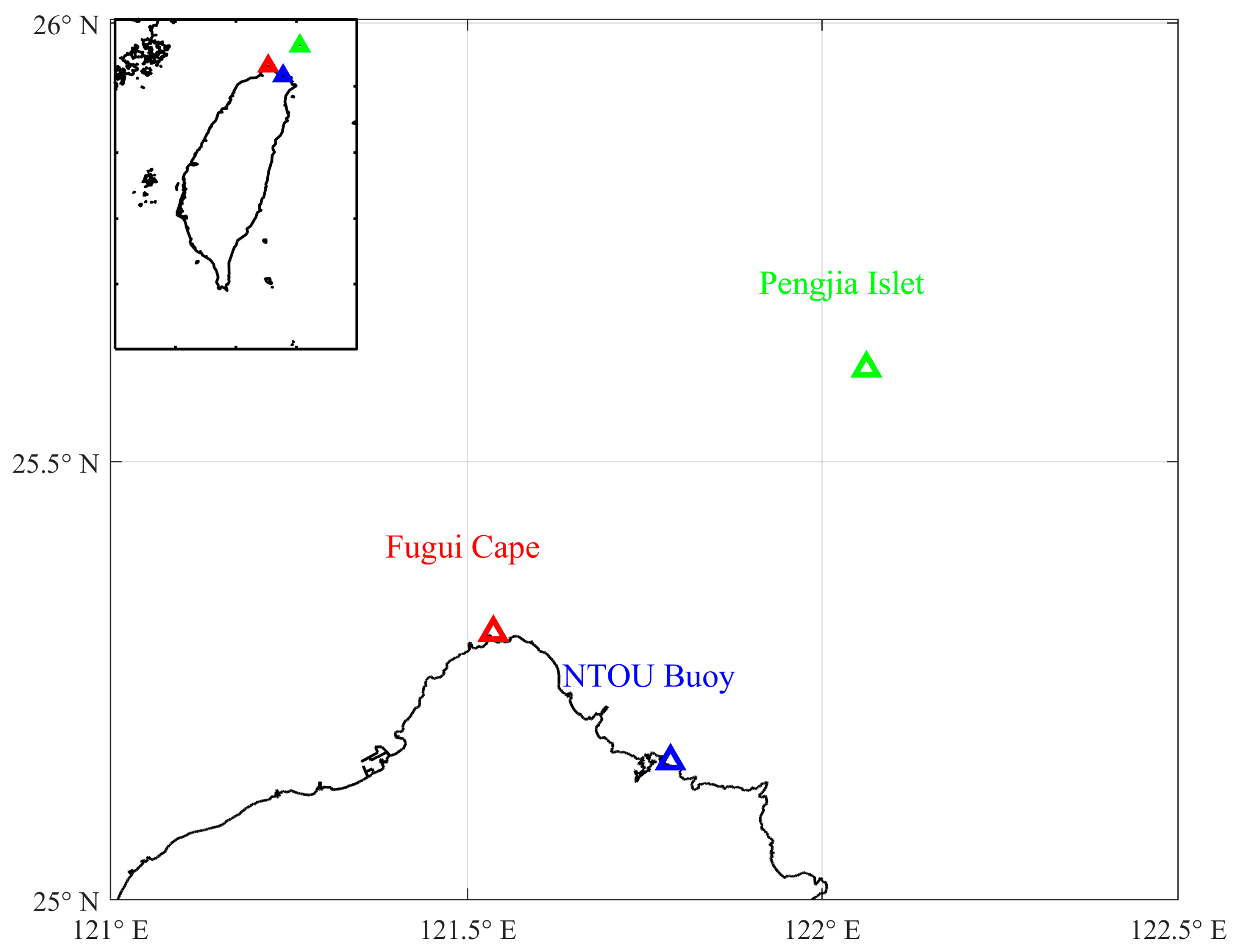
This study focuses on the northeast maritime region of Taiwan, which is influenced by the northeast monsoon from October to the following March. During this period, the winds are robust, with average speeds ranging from 5.5 to 17.1 m/s, exhibiting wind pow-er comparable to a tropical depression. Additionally, the water depth in this area is ap-proximately 30–50 m, making it an ideal site for developing wave energy and floating offshore wind power. The study collected detailed observational data from wave buoys installed by the Central Weather Bureau at Pengjia Islet and Fugui Cape and data buoys set up by the National Taiwan Ocean University (NTOU). The objective is to analyze these data comprehensively to gain a deeper understanding of the wave characteristics in this region. The specific locations and relevant information of the buoy stations are depicted in Figure 1 and Table 1. Notably, the marine energy test site of NTOU is the first real-sea test site in Taiwan.

Figure 1.
Location of measurement stations around the northeast coast of Taiwan.

Table 1.
Details of data measurement stations around northeast coasts of Taiwan.
The measurement ranges and resolutions of the wave buoys installed by the Central Weather Bureau are as follows: significant wave height: 0–20 m, resolution: 0.1 m; mean period: 3–30 s, resolution: 0.1 s; spectrum: 0.03–0.4 Hz, resolution: 0.01 Hz; directional measurement: 0–360 degrees. For the National Taiwan Ocean University wave buoy, the measurement ranges and resolutions are as follows: significant wave height: 0–20 m, resolution: 0.01 m; mean period: 1.5–33 s, resolution: 0.1 s; wave spectrum: 0.03–0.64 Hz, resolution: 0.005 Hz; directional measurement: 0–360 degrees.
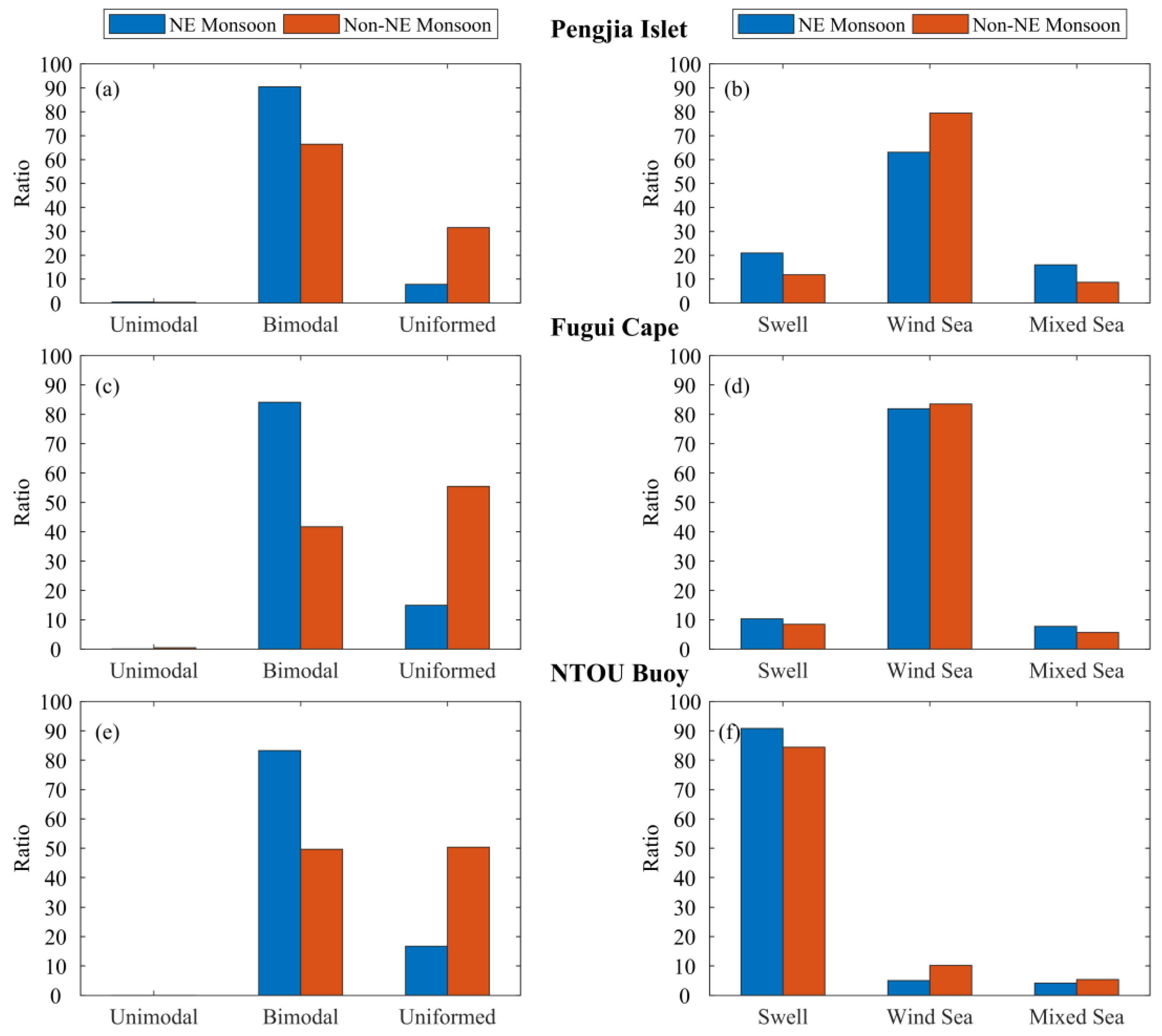
Figure 2 shows the analysis results of wave types at each station during northeast monsoon (blue column) periods and the non-northeast monsoon (orange column). The left figures illustrate unimodal, bimodal, and unformed spectra, while the figures on the right side depict swell-dominated, wind-wave-dominated, and mixed sea conditions. From top to bottom, the results correspond to Pengjia Islet, Fugui Cape, and the National Taiwan Ocean University buoy data.

Figure 2.
The ratio of wave type in the different stations: (a,b) Pengija Islet; (c,d) Fugui Cape; (e,f) NTOU Buoy.
The data from the Pengjia Islet station (Figure 2a) show that the unimodal spectra proportion is deficient (approximately 0.5%) during the northeast and non-northeast monsoon periods. Bimodal and unformed spectra account for 91.5% and 8% during the northeast monsoon. During the non-northeast monsoon period, the proportion of bimodal spectra decreases to 67%, while unformed spectra increase to 32.5%. Figure 2b results show that wind wave dominance prevails in the northeast and non-northeast monsoon periods (63% and 79.5%, respectively). On the other hand, the proportions of swell-dominated and mixed-sea conditions during the northeast monsoon are 21% and 16%, respectively; during the non-northeast monsoon, these proportions decrease to 12% and 8.5%.
The wave type statistics at Fugui Cape station (Figure 2c,d) are similar to those at Pengjia Islet. The proportion of unimodal spectra remains below 0.5% throughout the year. During the northeast monsoon, the proportions of bimodal and unformed spectra are 84.5% and 15%, respectively; however, during the non-northeast monsoon, the proportion of bimodal spectra drops to 41.7%, while unformed spectra increase to 57.8%. Figure 2d shows that wind wave dominance exceeds 80% during the northeast and non-northeast monsoon periods (82% and 84.5%, respectively). The proportions of swell-dominated and mixed-sea conditions during the northeast monsoon are 10.3% and 7.7%, respectively; during the non-northeast monsoon, these proportions decrease to 8.5% and 7%.
The results from the National Taiwan Ocean University data buoy are shown in Figure 2e,f. The results show (Figure 2e) that unimodal spectra are nearly absent in this region. During the northeast monsoon, the proportions of bimodal and unformed spectra are 83.3% and 16.7%, respectively. During the non-northeast monsoon, these proportions change to 49.7% and 50.3%, similar to the results from the Fugui Cape station. In terms of dominant wave types, due to the buoy’s closer proximity to the shore, swell-dominated conditions prevail. During the northeast and non-northeast monsoon, swell-dominated conditions are 90.8% and 84.4%, respectively. Wind-wave-dominated and mixed-sea conditions account for only 5% and 4.2%, respectively, for the northeast monsoon; these proportions increase for the non-northeast monsoon to 10.2% and 5.4%, respectively.
3. Spectrum Forms of the Frequency Spectrum and Fitting Technology
The method employed in this study to classify unimodal, bimodal, or non-specific spectra begins with identifying the positions of local minima and maxima. Subsequently, it assesses whether there are one or two peaks within these intervals. If no peaks are found, or spectral energy is less than 0.5 m2s, it is defined as a non-specific spectrum. To determine whether the spectrum belongs to swell, wind waves, or a combination of both, we utilize the separation frequency method proposed by Gilhousen and Hervey [41]:
where fu and fl represent the upper and lower bounds of frequency, S is the spectrum, g is the gravitational acceleration, and the separation frequency fs can be defined as
In the Equation (2), fx represents the maximum value obtained from the ξ(fl) calculation. Further classification is conducted based on the indicator SSER proposed by Rodriguez and Guedes Soares [42]:
SSER < 0.8, 0.8 ≤ SSER < 1.2, and SSER ≥ 1.2 can be distinguished as swell-dominated, mixed-sea dominated, and wind wave-dominated.
3.1. Unimodal Wave Spectrum
This study utilizes the JONSWAP, PM, TMA, Wallop, and JW spectral models, and their respective equations are presented as follows:
3.1.1. JONSWAP Spectrum
The JONSWAP spectrum is developed based on the Joint North Sea Wave Project’s in situ data to describe the spectrum in the growth and fully developed stages of waves [12], i.e.,
where f and fp are the frequency and peak frequency, and γ is the spectral peak enhancement factor. In addition, σ = 0.07 when f ≤ fp and σ = 0.09 when f > fp.
3.1.2. Pierson–Moskowitz (PM) Spectrum
The Pierson–Moskowitz spectrum is a particular case of the JONSWAP spectrum where the spectral peak enhancement factor γ equals 1 and written as
3.1.3. TMA Spectrum
Bouws et al. [13] introduced the TMA spectrum, an extension of the JONSWAP concept suitable for finite water depth, i.e.,
where k and h are the wave number and water depth, respectively.
3.1.4. Wallop Spectrum
Huang et al. [19] proposed the Wallop spectrum, which is suitable for describing waves in the development, fully developed, and decay stages, i.e.,
where is the gamma function, β is the spectrum shape coefficient, and m is the high-frequency tail shape parameter.
3.1.5. JW Spectrum
Gao et al. [20] combined the JONSWAP and Wallop spectra, adjusting the spectral peak value with JONSWAP’s peak enhancement factor (γ) and making the overall spectrum more versatile and flexible with Wallop’s m value, i.e.,
3.2. Bimodal Wave Spectrum
3.2.1. Ochi–Hubble Spectrum
Ochi and Hubble [32], based on the wind-wave spectrum proposed by Kitaigorodskii [18,43], utilized a Gaussian distribution assumption for sea surface variations (indicating a correlation with significant wave height) and introduced the sharpness parameter λ to control the spectral sharpness. When describing a bimodal spectrum where both wind and swell wave systems coexist, the assumption is made that the wind and swell wave spectra are linearly superposing, as illustrated in Equation (11):
where Hs is significant wave height, fp is peak frequency, and λ is the sharpness parameter. The subscripts j = 1 and 2 represent swell and wind-wave systems, respectively.
3.2.2. Torsethaugen Spectrum
The Torsethaugen spectrum is primarily a dual-peak spectrum model that combines two JONSWAP spectra, as expressed in Equation (12).
Here, the subscripts j = 1 and 2 represent the main wave peak system and the secondary wave peak system, respectively. Ej is the weight function, and Sjn(fjn) is the JONSWAP-spectrum, which can be expressed as follows:
where Hj, Tp, and Aγ represent significant wave height, peak period, and spectral shape parameters, respectively. The parameters in Equations (13)–(15) are determined by the prevailing sea conditions and can be further referenced in Torsethaugen [30].
3.3. Fitting Method and Evaluation Index
The least squares method is an essential mathematical approach for data processing and error assessment. Achieving the best fit between a model and a set of samples involves collecting partial sample data to fit a specific model. Generally, the least squares method estimates model parameters based on minimizing the sum of squared errors. Assuming the model function is denoted as f(x), the actual observed values as yi, and the model predicted values as f(xi), this method can be expressed as follows:
where x is a vector composed of parameters in the model, and e(x) is the residual vector. When the function f(x) is expressed as a nonlinear relationship in terms of x, it is referred to as the nonlinear least squares method.
In order to assess the fitting results, this study adopts the correlation coefficient (cc) and root mean square error (rmse) as evaluation indices. The correlation coefficient is based on the deviations of two variables from their means. It primarily reflects the degree of correlation between the fitted and measured spectrum, as shown in Equation (18). When the computed result is close to 1.0, it indicates a stronger correlation between the two curves. The root mean square error measures the accuracy of the fit between the modeled spectrum and the measured spectrum (as shown in Equation (19)); a value closer to 0 indicates a higher degree of data fit.
where N is the total number of data points, Sm and So represent the fitted and measured spectrum results, and Sm and So denote the respective mean values of the fitted and measured spectrum.
4. Results and Discussion
This study employs various wave spectrum models to investigate wave data through Pengjia Islet, Fugui Cape, and the NTOU wave buoy. The aim is to determine the most suitable unimodal and bimodal wave spectrum models. Section 4.1 examines the applicability of unimodal wave spectrum models at different stations. Section 4.2 explores the applicability of bimodal wave spectrum models at different stations. Section 4.3 investigates the characteristics and spectral parameters of waves during the northeast and non-northeast monsoon periods. Section 4.4 discusses the application of wave spectrum parameters to the NTOU wave buoy.
4.1. Unimodal Wave Spectra (JONSWAP, PM, TMA, Wallops, and JW)
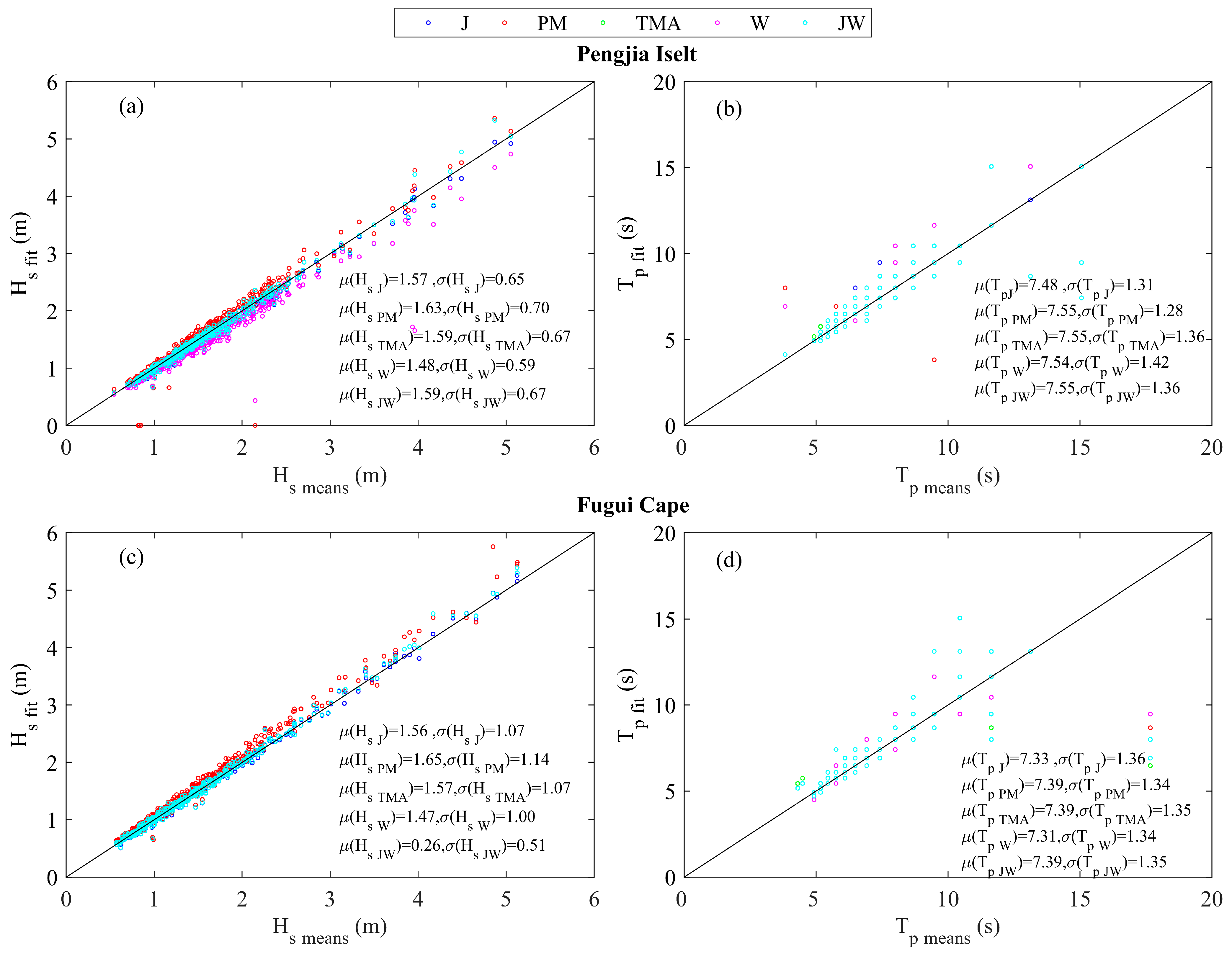
This section evaluates the suitability of different unimodal wave spectra for the Pengjia Islet and Fugui Cape monitoring stations in the northeast coastal waters of Taiwan. Figure 3 represents the fitting results and observed significant wave height (Hs) and peak period (Tp) values for the Pengjia Islet and Fugui Cape stations.
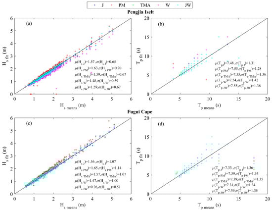
Figure 3.
Comparison of Hs and Tp of each fitting model and measured results for unimodal wave spectrum: (a,b) Pengjia Islet; (c,d) Fugui Cape.
Regarding Hs (as shown in Figure 3a,c), the fitting results at both the Pengjia Islet and Fugui Cape stations exhibit a distribution along the 45-degree line, indicating good performance for all the models. However, there are apparent discrepancies between the fitting results and observations of Tp (Figure 3b,d). Overall, the JONSWAP wave spectrum provides a better fit. Moreover, at the Pengjia Islet station, the standard deviation of Hs falls roughly between 0.59 and 0.70 m, with the Wallop model having the lowest. The indicative wave period Tp ranges from 1.28 to 1.42 s, with the PM model having the lowest value. The Fuguei Cape station’s standard deviation of Hs ranges from 0.51 to 1.14 m, with the JW model performing the best. The standard deviation of Tp is quite close, ranging from 1.34 to 1.36 s.
Figure 4a,b illustrate the proportions of the best-fitting wave spectrum models for the Pengjia Islet and Fugui Cape stations, respectively. Figure 4a shows that the JONSWAP wave spectrum model best fits the Pengjia Islet station, accounting for 43.75% of the total, because this station is located closer to the open sea, where wind-driven waves predominantly influence the conditions. On the other hand, Figure 4b shows the results for the Fugui Cape station, where the TMA wave spectrum model is predominant in the best-fitting results (31.5%). Owing to the station’s proximity to the nearshore area, the limited water depth makes the TMA wave spectrum model a better fit for the observed data.
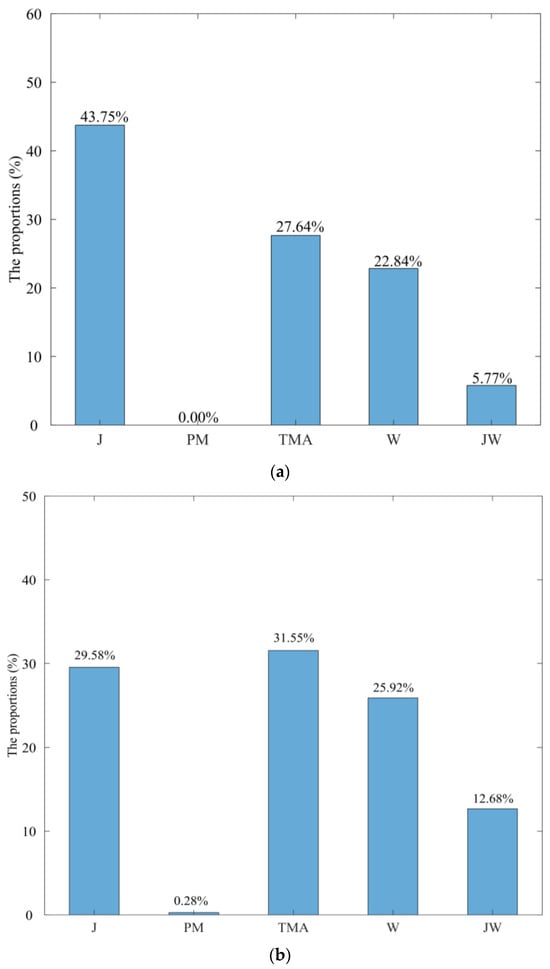
Figure 4.
The optimal fitting proportion of each unimodal spectrum at (a) Pengjia Islet station and (b) Fugui Cape station.
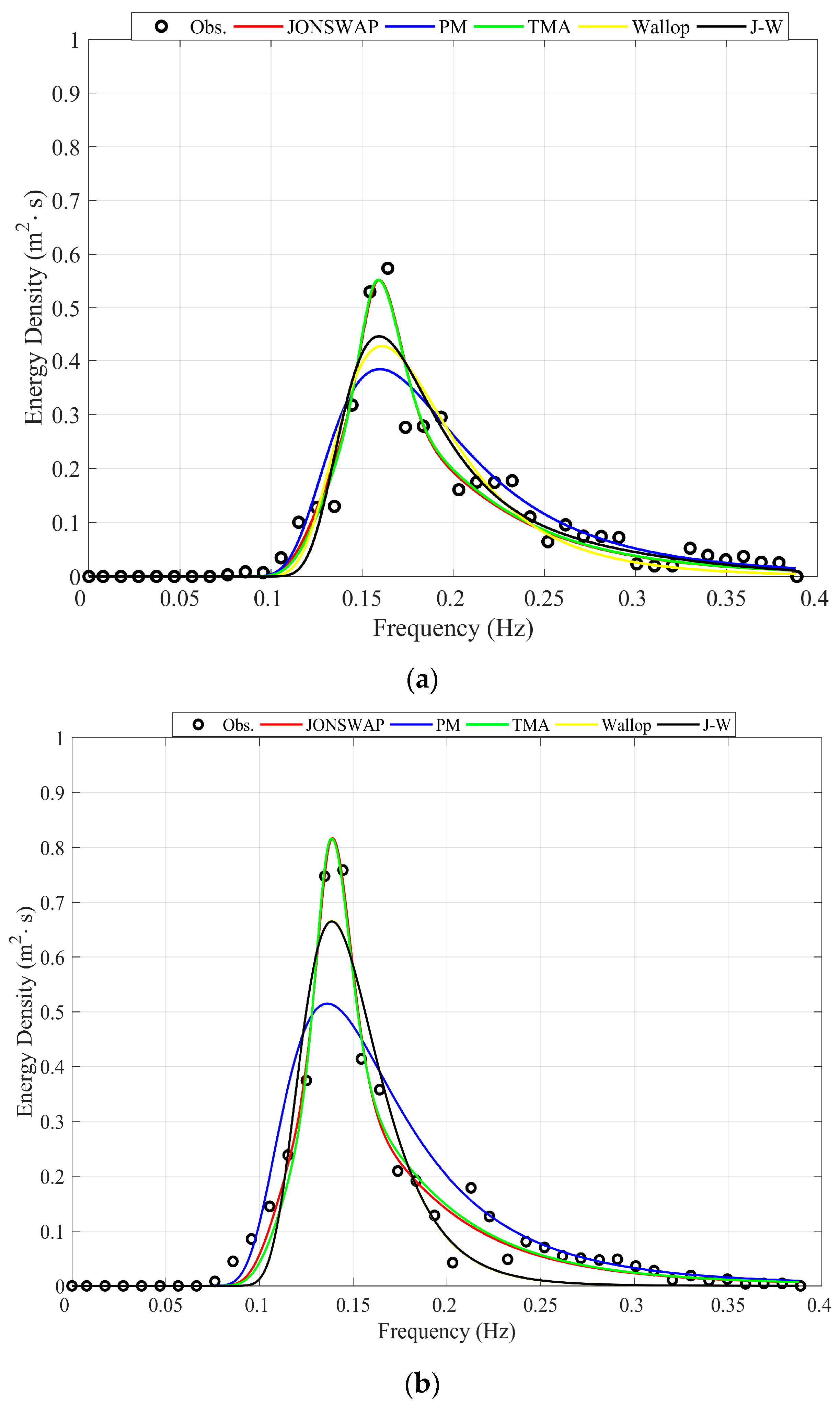
Figure 5a,b present the fitting results of different unimodal wave spectrum models at the Pengjia Islet and Fugui Cape stations, respectively. The results indicate that, for the Pengjia Islet station, the JONSWAP wave spectrum better describes the variations in the wave spectrum. For the Fugui Cape station, the JONSWAP and TMA wave spectrum models provide better descriptions of the fitting results. The integrated areas of the observed values and various spectral models were compared to investigate the differences among spectra further. After integrating the results from the Pengjia Islet station in Figure 5a, the area of the observed spectrum is 0.0390 Hz·m2s. The integrated areas for the JONSWAP, PM, TMA, Wallop, and JW models are 0.381, 0.381, 0.381, 0.355, and 0.366 Hz·m2s, respectively. Figure 5b at the Fuguei Cape station shows the observed spectrum area of 0.448 Hz·m2s. The corresponding integrated areas for the JONSWAP, PM, TMA, Wallop, and JW models are 0.427, 0.427, 0.427, 0.372, and 0.372 Hz·m2s, respectively. The above results show that the JONSWAP, PM, and TMA models provide results closest to the observed values. However, while consistent with the other two models, the PM model exhibits lower sharpness, resulting in an overall lower correlation than the other two models. Although the JW model showed relatively good fit percentages of 5.77% and 12.68% in Figure 4, its performance in comparing integrated areas with observed values is relatively poor.
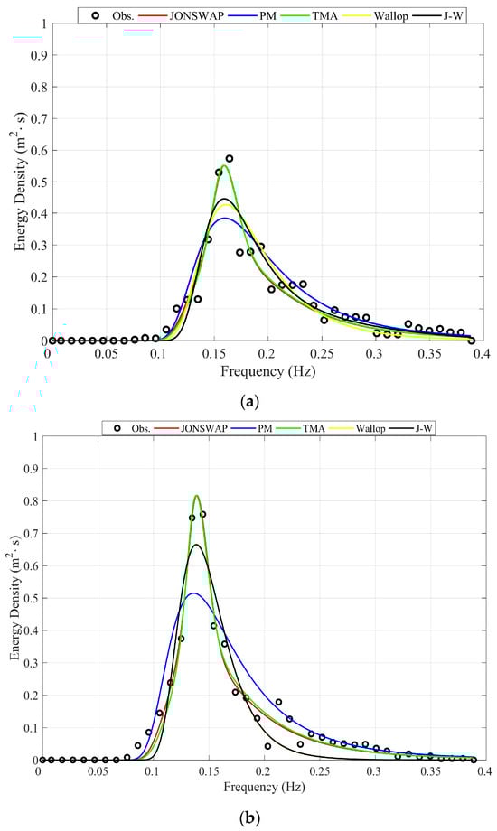
Figure 5.
Comparison of each fitting model and measured results of unimodal spectra (a) in Pengjia Islet at 1400 14 August 2021 and (b) in Fugui Cape at 0500 16 April 2016.
4.2. Bimodal Wave Spectra (OH, TH, and JW-J)
This section evaluates the fitting results of different bimodal wave spectrum models at the Pengjia Islet and Fugui Cape stations. Previous studies have indicated that the characteristic parameters may differ in other regions even if the spectrum models are similar [30]. Therefore, this study aims to propose a bimodal wave spectrum model suitable for the waters off the northeast coast of Taiwan.
Initially, this research adopts the JW spectrum, which can comprehensively describe different stages of waves for the low-frequency wave part (swell system). For the high-frequency wave spectrum part (wind wave system), the JONSWAP spectrum is employed. The primary reason is that it consistently yields good results when describing wind wave spectra in different regions. The following equation presents the linear superposition of these two spectra:
where m is the shape parameter, fs and fw represent the frequencies of swell and wind waves, and γw is the spectral peak enhancement factor for wind waves.
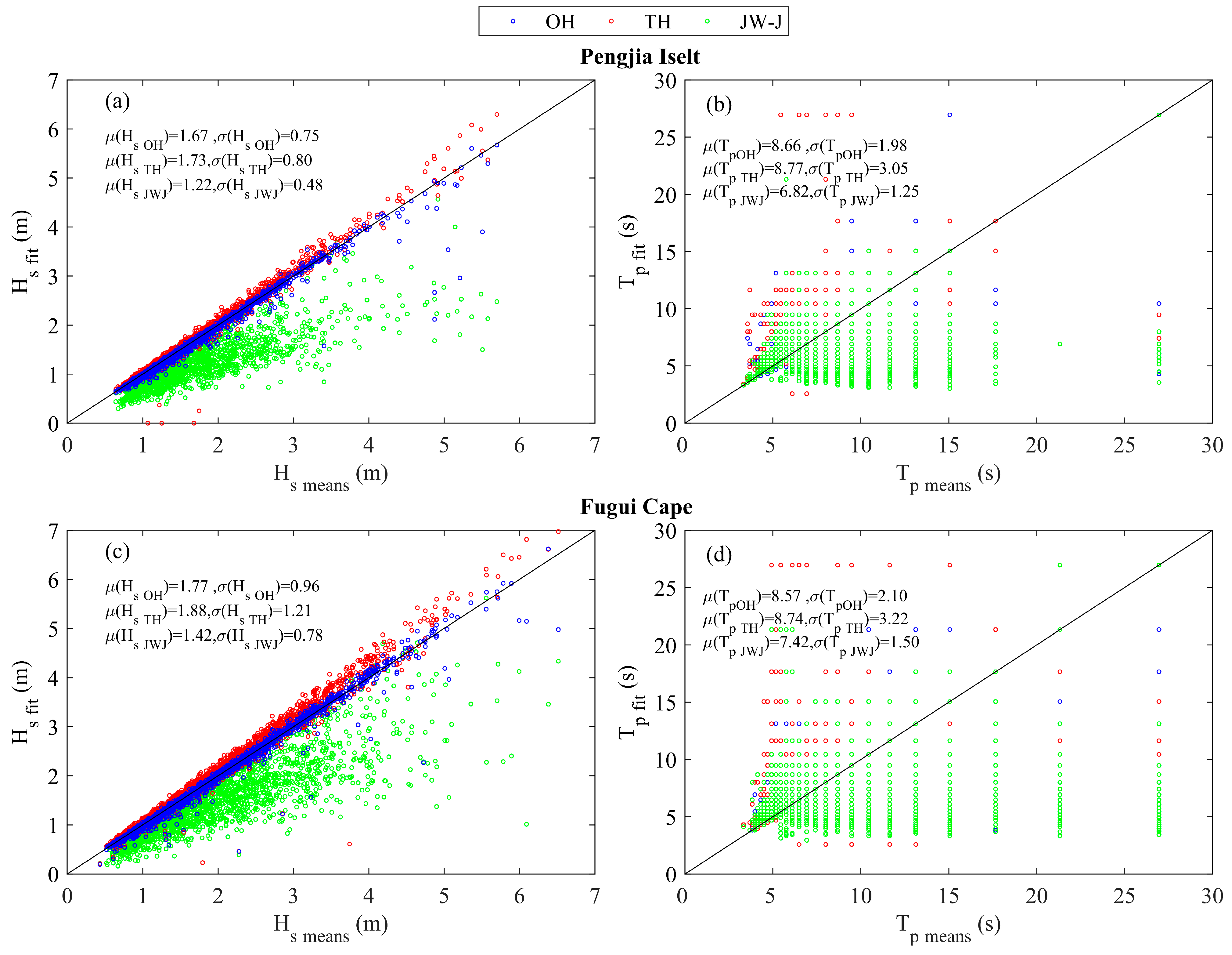
Figure 6 presents the fitting results of different bimodal wave spectrum models applied to the Pengjia Islet and Fugui Cape stations, along with observed Hs (Figure 6a,c) and Tp (Figure 6b,d). The JW-J spectrum tends to underestimate Hs in both the Pengjia Islet and Fugui Cape stations (green circles), particularly as wave height increases. In contrast, results from the OH spectrum (blue circles) exhibit good performance. The TH spectrum (red circles) performs relatively well, but some results scatter near zero. Both stations show differences between fitting and predicted results in peak period parts. It can also be observed that, at the Pengjia Islet station, the standard deviation of Hs for bimodal spectra falls roughly between 0.48 and 0.75 m, with the JW-J model proposed in this study having the lowest. The indicative standard deviation of wave period Tp ranges from 1.25 to 3.05 s, with the TH model exhibiting a more significant deviation. As for the Fugu© Cape station’s standard deviation of Hs, it ranges from 0.78 to 1.21 m, with the JW-J model still performing the best. The standard deviation of Tp is situated between 1.50 and 3.22 s.
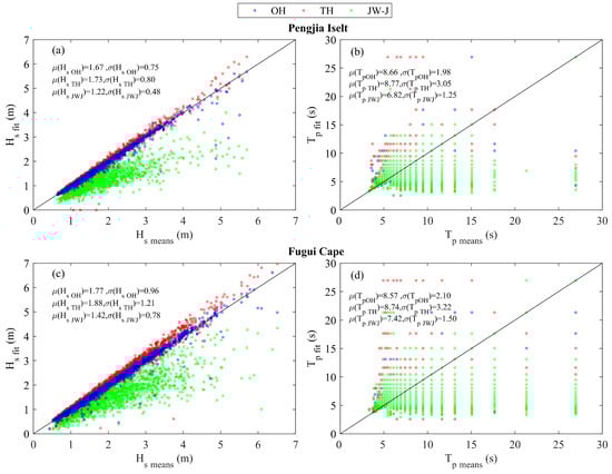
Figure 6.
Comparison of Hs and Tp of each fitting model and measured results for bimodal wave spectrum: (a,b) Pengjia Islet and (c,d) Fugui Cape.
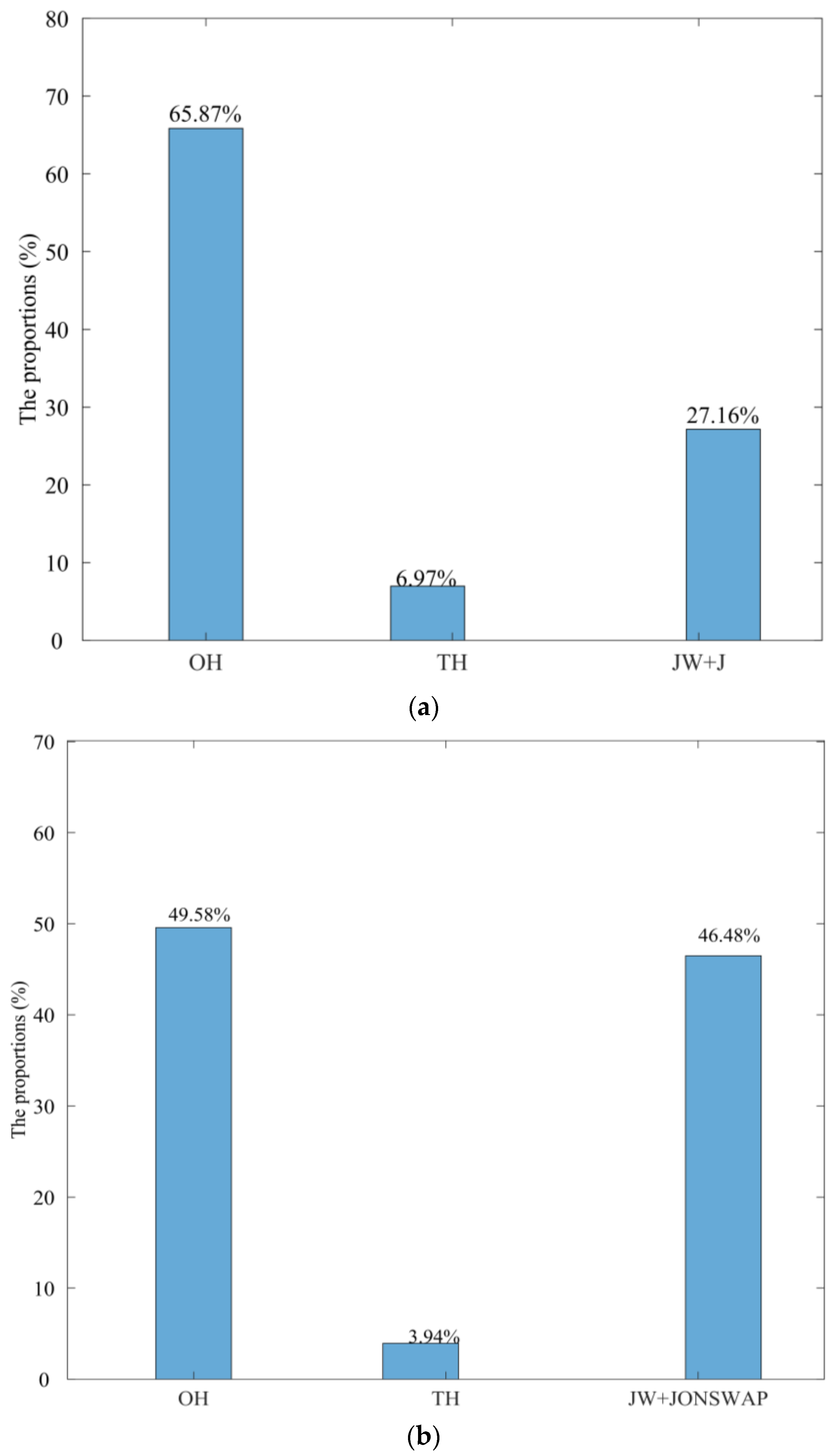
Figure 7a,b illustrate the proportions of optimal fitting results for each bimodal wave spectrum model at the Pengjia Islet and Fugui Cape stations. From the results in Figure 7a, it can be observed that the optimal spectrum model for Pengjia Islet is OH, accounting for 65.87%. The proposed JW-J spectrum in this study represents 27.16%. Owing to the deeper water depth in this region, the influence of nearshore conditions is less pronounced, and it aligns with the assumption of the OH spectrum that sea surface fluctuations follow a Gaussian distribution. For the Fugui Cape station (see Figure 7b), although the OH spectrum still dominates the optimal fitting results at 49.58%, the proposed JW-J spectrum is close behind at 46.48%. The reason may be that the station is located closer to the coast, where the JW-J spectrum better describes the characteristics of low-frequency waves in different wave stages, resulting in a good fit. The TH spectrum represents only 6.97% and 3.94% at the two stations, consistent with previous research findings [15]. Despite the TH spectrum being validated with measured data on the Norwegian coast, its model parameters may need adjustment for different regions to achieve better fitting results.
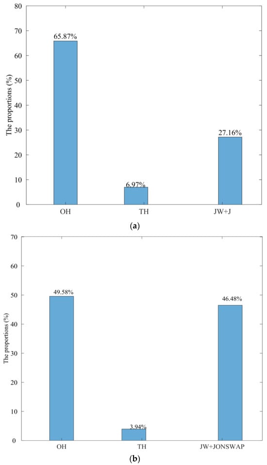
Figure 7.
The optimal fitting proportion of each bimodal spectrum at (a) Pengjia Islet station and (b) Fugui Cape station.
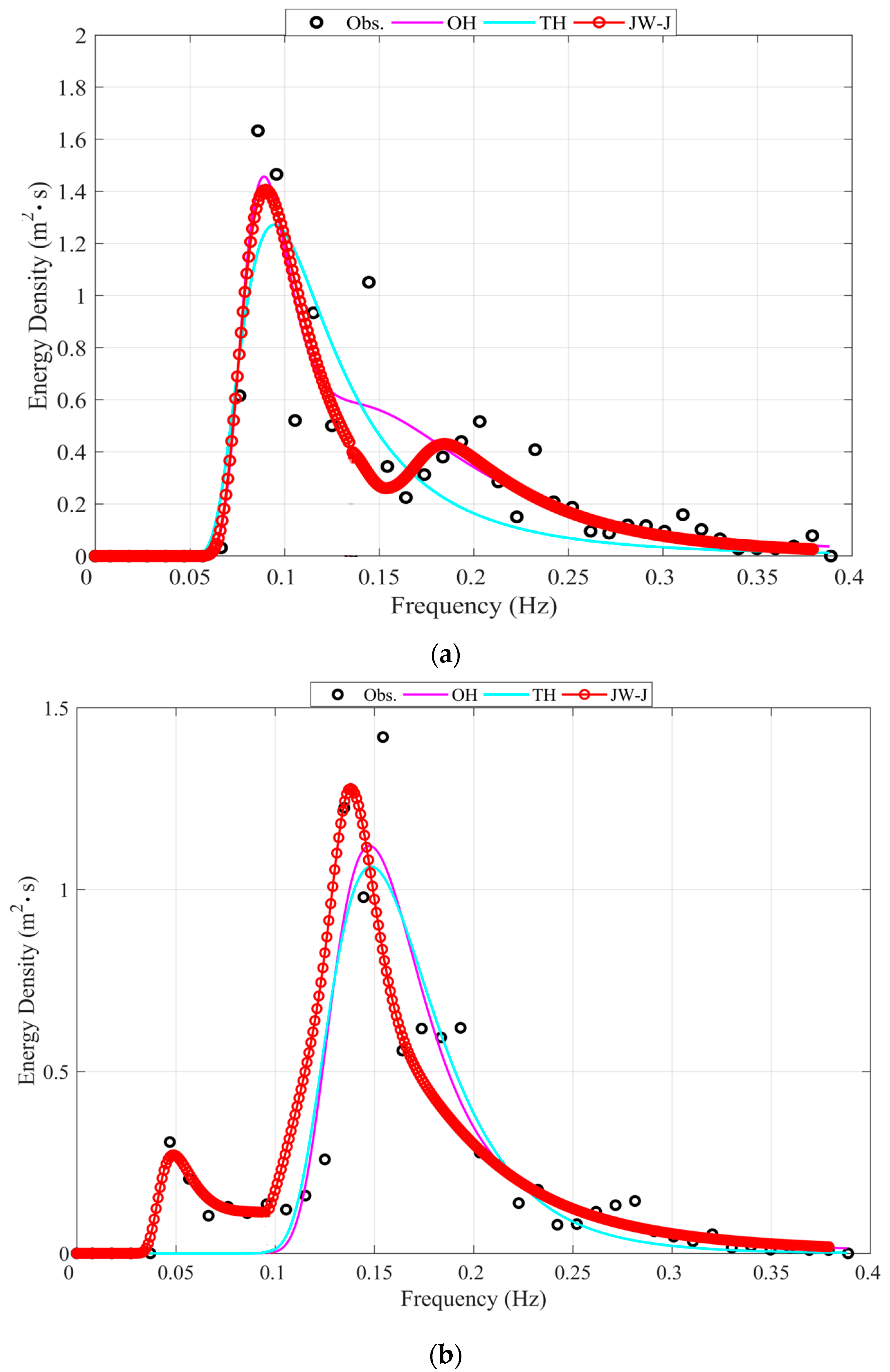
Figure 8a,b present the fitting results of different bimodal wave spectrum models at the Pengjia Islet and Fugui Cape stations. In the case of Pengjia Islet, the wind-wave system has more energy, and the energy of the swell system is relatively weaker. Figure 8a shows that OH and JW-J spectra closely match the measured data. In contrast, the TH spectrum tends to be underestimated, especially in the high-frequency (wind wave system) part. For the Fugui Cape station, the energy of the swell system is relatively stronger, and the wind wave system is weak. According to the results in Figure 8b, the OH spectrum effectively captures the variations in the measured spectrum. However, there needs to be more underestimation in the high-frequency (wind wave system) part. The JW-J spectrum effectively fits the measured data at low and high frequencies, while the TH spectrum exhibits an overall underestimation trend.

Figure 8.
Comparison of each fitting model and measured results of bimodal spectra (a) in Pengjia Islet at 1000 1 January 2021 and (b) in Fugui Cape at 1700 04 Jun 2016.
4.3. Spectral Shape Parameter (m, γw)
To analyze the wave characteristics of a specific region, in addition to examining the basic parameters of waves, such as Hs and Tp, the analysis of spectral parameters is also crucial for describing wave-spectrum models. Adjusting spectral parameters allows for a better representation of local features in the spectrum to align with actual observational data. When controlling the shape of the JW-J spectrum, consideration is typically given to the swell system’s spectral tail shape parameter (m) and the peak enhancement factor for the wind wave system (γw).
In northeastern Taiwan, the northeast monsoon influences the region every October to next March, providing a stable wave energy source. Therefore, analyzing and comparing periods influenced by the northeast monsoon and those not influenced by it is necessary to understand wave characteristics comprehensively.
4.3.1. Northeast Monsoon Period
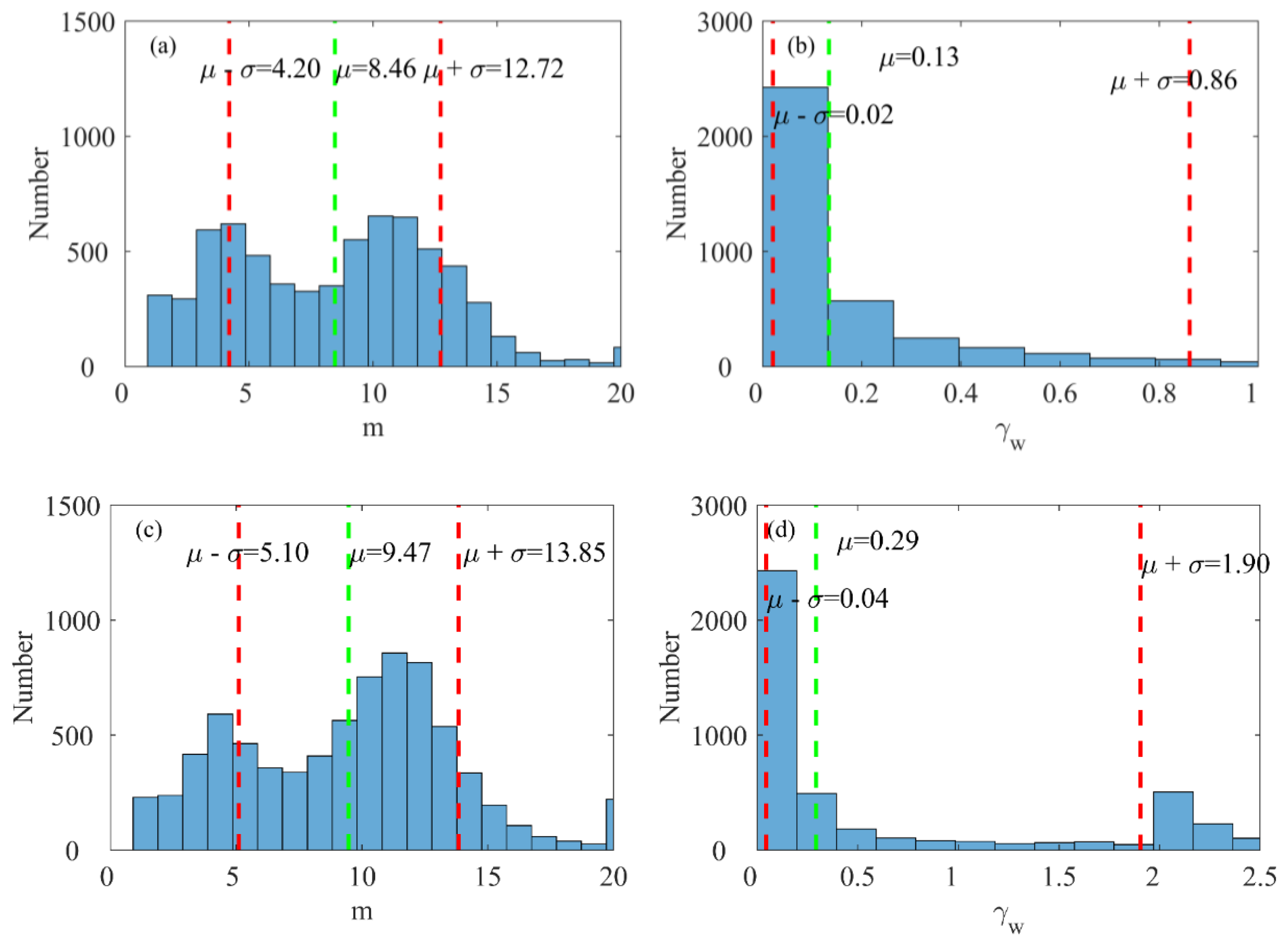
Figure 9 presents the distribution of shape parameter m (shown in Figure 9a) and spectral peak enhancement factor γw (see Figure 9b) during the northeast monsoon period at the Pengjia Islet station. The red dashed lines represent one standard deviation range, and the green dashed lines represent the mean values. Table 2 presents the wave characteristics and spectral parameters for different periods at each station. Table 3 shows the performance of different spectra models during the northeast monsoon period (here, Hs and Tp are defined within one standard deviation range). For the Pengjia Islet station, the one standard deviation range for Hs and Tp is 1.03 m to 2.47 m and 5.75 s to 7.41 s, respectively—the corresponding values for m and γw range from 4.35 to 12.41 and 0.01 to 0.37.
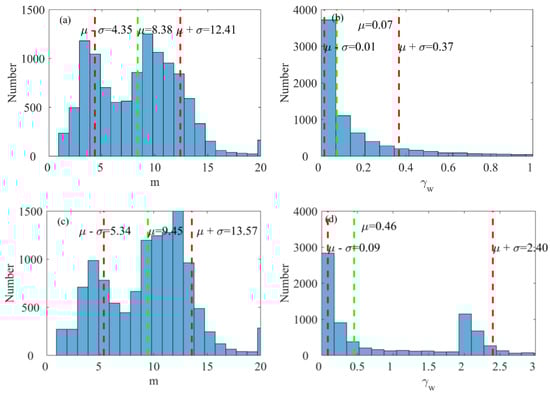
Figure 9.
The statistics distribution of the shape parameter m and the peak enhancement factor γω during northeast monsoon: (a,b) in Pengjia Islet; (c,d) in Fugui Cape.
Table 2.
Characteristics and parameters of wave at different stations during northeast and non-northeast monsoon periods.
Table 3.
The performance of different spectra models during the northeast monsoon period.
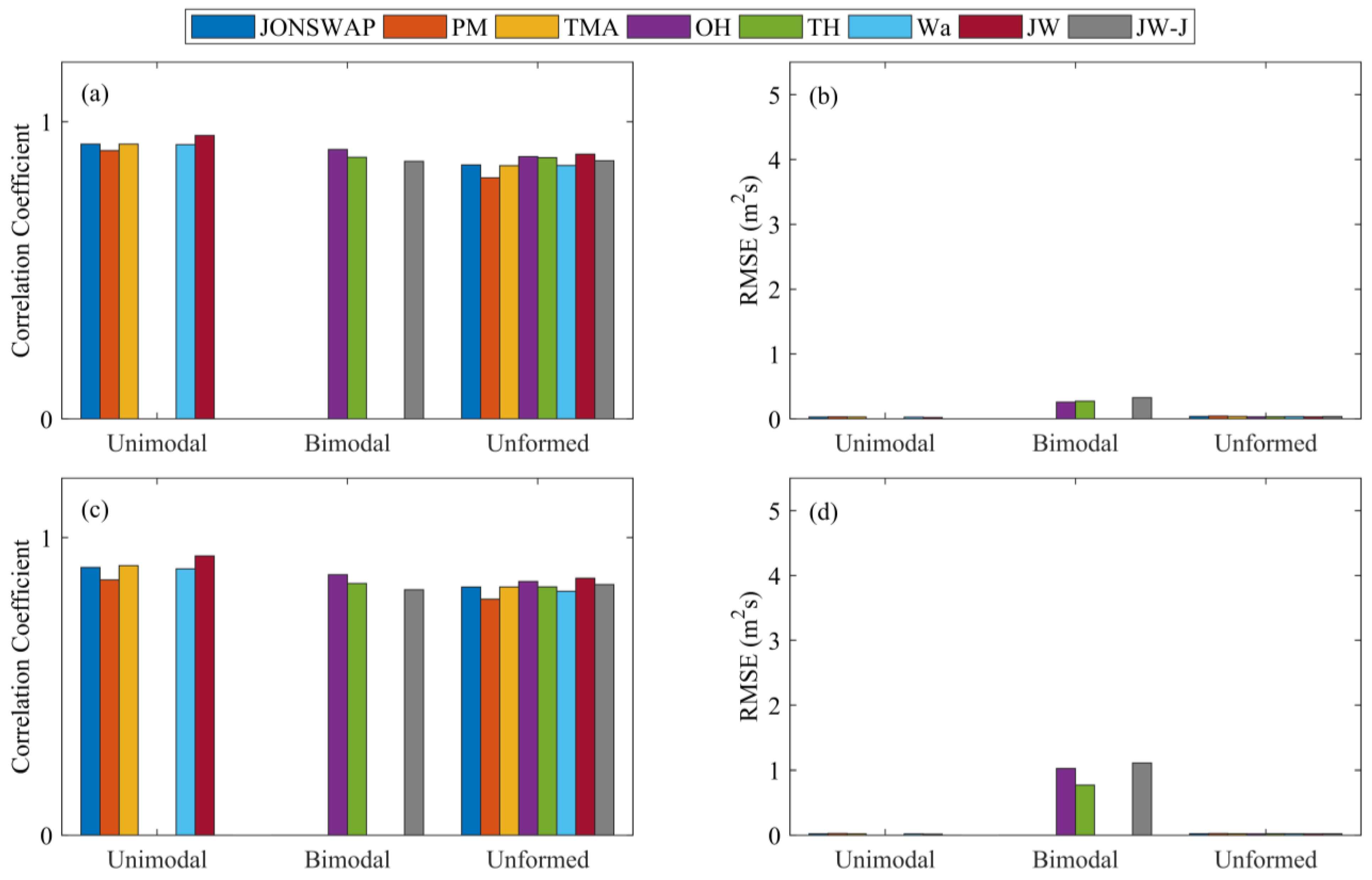
Figure 10a shows the correlation coefficients (cc) and root mean square error (rmse) results when applying different spectrum models to the Pengjia Islet station. For the unimodal spectrum, the JONSWAP spectrum (blue column) and JW spectrum (dark red column) perform the best (cc are 0.940 and 0.952 and rmse are 0.05 m and 0.10 m, respectively). In the case of bimodal spectra, the OH spectrum (purple column) exhibits the best performance with cc and rmse values of 0.930 and 0.353 m. The cc and rmse of the JW-J spectrum model (gray column) are 0.837 and 0.592 m, respectively.
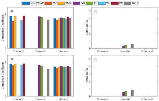
Figure 10.
The performance of each spectrum model during the northeast monsoon period: (a,b) in Pengjia Islet; (c,d) in Fugui Cape.
Figure 9b shows the distribution of shape parameter m and spectral peak enhancement factor γw at the Fugui Cape station during the northeast monsoon period. At Fugui Cape, the one standard deviation range for Hs and Tp is 0.78 m to 2.79 m and 6.09 s to 8.68 s, respectively—the corresponding values for m and γw range from 5.34 to 13.57 and 0.09 to 2.40.
Figure 10b presents the cc and rmse results when applying different spectrum models to the Fugui Cape station. The results are like those for Pengjia Islet. The JONSWAP and JW spectra perform better for unimodal spectra, while the PM spectrum (orange column) performs the worst. The OH spectrum (purple column) performs best for bimodal spectra, with cc and rmse values 0.911 and 0.54 m, respectively. In terms of the JW-J spectrum model (gray column), the correlation coefficient (cc) and root mean square error (rmse) display 0.800 and 0.86 m, respectively.
4.3.2. Non-Northeast Monsoon Period
Figure 11a illustrates the distribution of the shape parameter m and the spectral peak enhancement factor γw at the Pengjia Islet station during the non-northeast monsoon period. The wave characteristics and spectral parameters for each station are presented in Table 2. Table 4 shows the performance of different spectra models during the northeast monsoon period. At the Pengjia Islet station, the one standard deviation range for Hs and Tp is 0.65 m to 1.71 m and 5.45 s to 7.42 s, respectively. The magnitude of Hs is reduced by approximately 1 m compared to the northeast monsoon period—the corresponding values for m and γw range from 4.20 to 12.72 and 0.02 to 0.86. The changes in spectral parameters are not apparent.

Figure 11.
The statistics distribution of the shape parameter m and the peak enhancement factor γω during non-northeast monsoon: (a,b) in Pengjia Islet, (c,d) in Fugui Cape.
Table 4.
The performance of different spectra models during the non-northeast monsoon period.
Figure 12a shows the correlation coefficients (cc) and root mean square error (rmse) results when applying different spectrum models to the Pengjia Islet station. For the unimodal spectrum, the JONSWAP spectrum (blue column) and JW spectrum (dark red column) perform the best (cc of 0.925 and 0.955 and rmse of 0.028 m and 0.022 m, respectively). In the case of bimodal spectra, the OH spectrum (purple column) exhibits the best performance with cc and rmse values of 0.906 and 0.258 m. The JW-J spectrum (gray column) has cc and rmse values of 0.867 and 0.326 m, respectively.
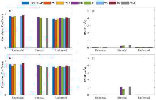
Figure 12.
The performance of each spectrum model during the non-northeast monsoon period: (a,b) in Pengjia Islet; (c,d) in Fugui Cape.
Figure 11b displays the distribution of the shape parameter m and spectral peak enhancement factor γw at the Fugui Cape station during the non-northeast monsoon period. The one standard deviation range for Hs and Tp is 0.34 m to 1.40 m and 5.17 s to 7.42 s—the corresponding values for m and γw range from 5.10 to 13.85 and 0.04 to 1.90. It is noticeable that the range of Hs and Tp at Fugui Cape differs from that at Pengjia Islet, resulting in variations in corresponding spectral parameter factors.
Figure 12b presents the correlation coefficients (cc) and root mean square error (rmse) results when applying different spectrum models to the Fugui Cape station during this period. The analysis results are similar to those at Pengjia Islet. The JONSWAP and JW spectra perform better for unimodal spectra, while the PM spectrum (orange column) performs the worst. The OH spectrum (purple column) performs best for bimodal spectra, with cc and rmse values of 0.876 and 1.02 m. The cc and rmse of the JW-J spectrum (gray column) show the values of 0.825 and 1.10 m, respectively.
4.4. Application of Spectral Parameters in Ocean Energy Testing Site
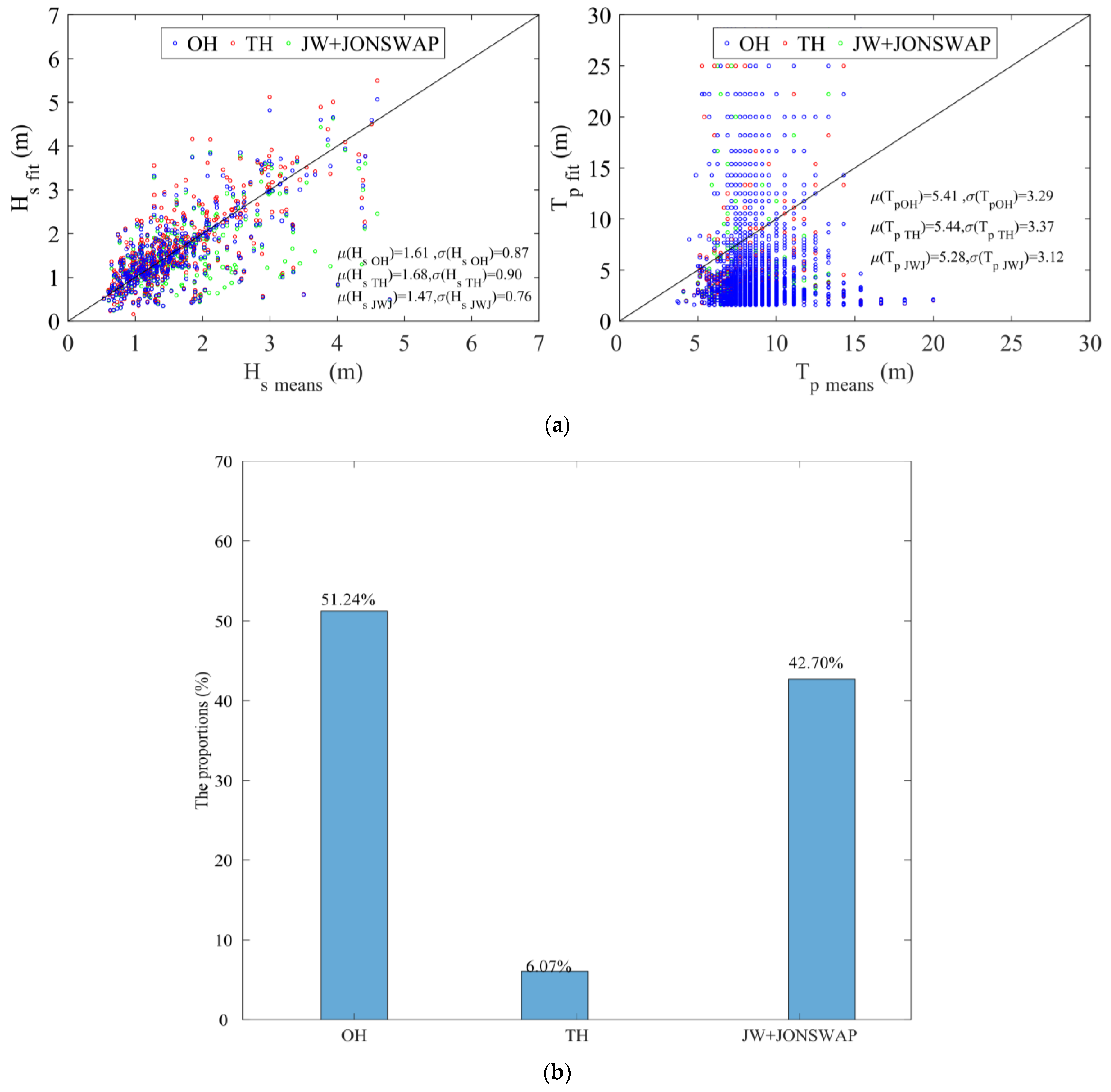
The wave buoy at NTOU is located between the Pengjia Islet station and the Fugui Cape station and is closer to the nearshore. How the JW-J spectrum model and its spectrum parameters are applied to this location is an essential contribution of this study. First, it is observed that the region exhibits a bimodal wave spectrum from Figure 2. Therefore, the results are shown in Figure 13a using a bimodal spectrum to fit the Hs and Tp. In terms of Hs, the fitting results of the JW-J spectrum (green circles) are closer to the measured values. However, there is an apparent discrepancy between the fitted and measured results for the Tp, similar to those at the other two stations. Overall, at the NTOU station, the standard deviation of Hs for bimodal spectra ranges from 0.76 to 0.90 m, with the JW-J model having the lowest. There is a relatively significant difference in the standard deviation of Tp (ranging from 3.12 to 3.37 s).
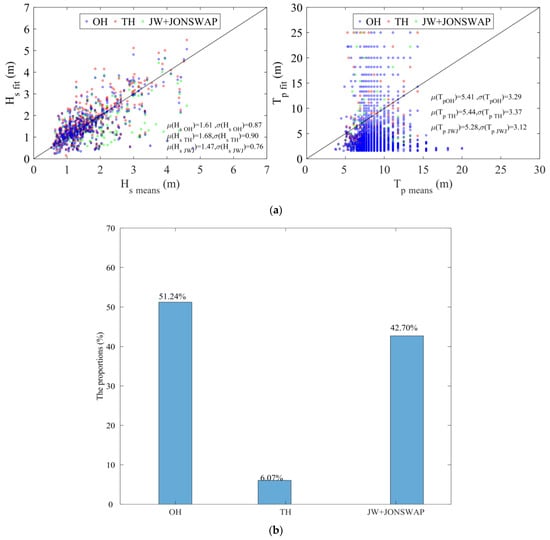
Figure 13.
(a) Comparison of Hs and Tp of each fitting model and measured results; (b) the optimal fitting proportion of each spectrum model at NTOU buoy station.
Figure 13b displays the proportion of the best-fitting results for various bimodal wave spectra models at the NTOU station. The optimal bimodal spectrum is the OH spectrum, accounting for 51.24%, followed by the JW-J spectrum, which accounts for 42.70%. Like the results at the other two stations, the TH spectrum performs the least favorably, with only 6.07%.
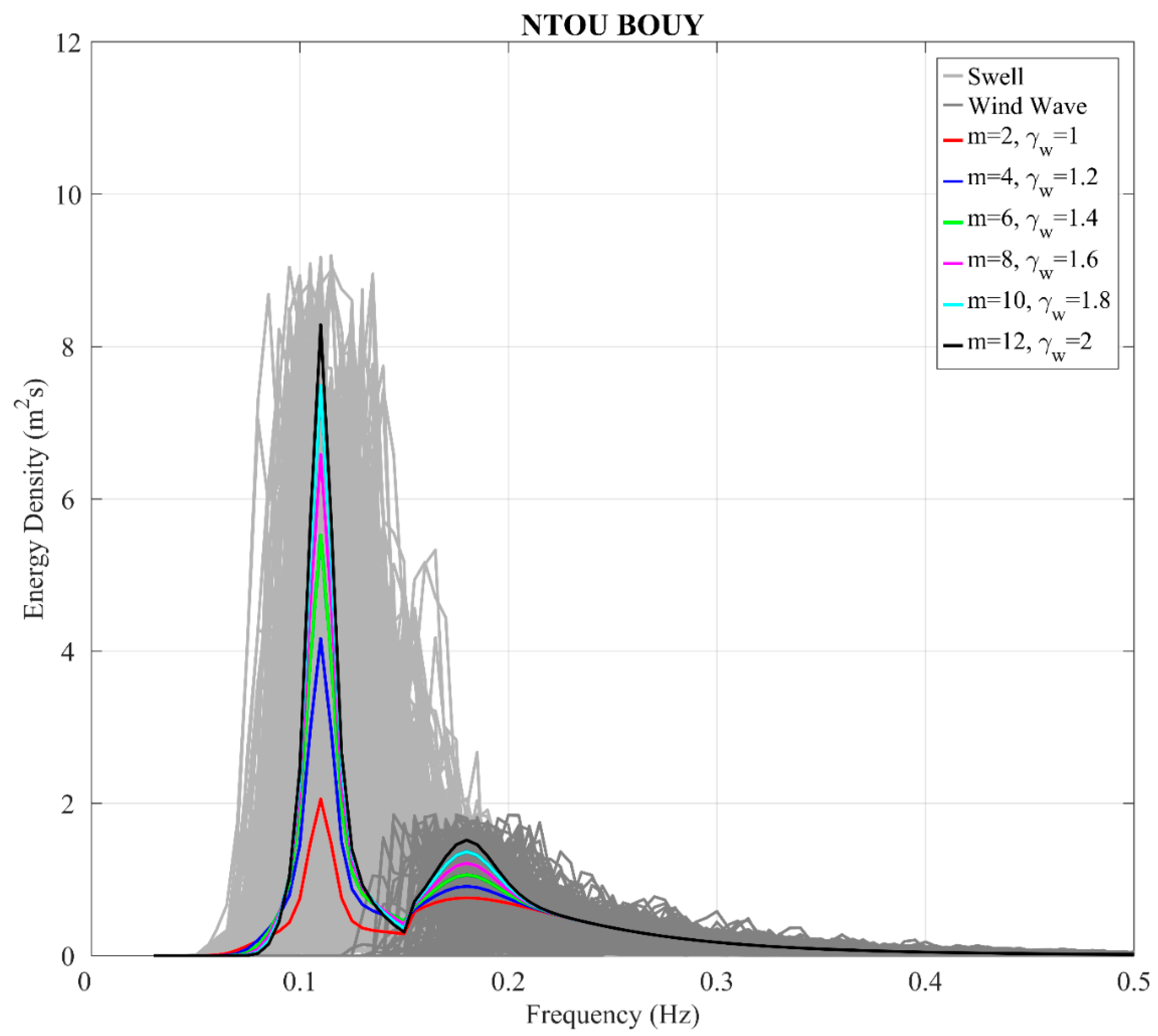
Figure 14 illustrates the variation of the JW-J spectrum with fixed parameters. The light gray and dark gray backgrounds represent the energy spectrum distribution of the swell and wind wave systems at the NTOU wave buoy. It can be observed that the energy of swells is stronger in this region, consistent with the dominance of swells in the wave patterns. Regarding the parameters of the JW-J spectrum, the assumption of Hs is 1.0 m, and the Tp for swell and wind waves are 10 s and 5.6 s, respectively. The shape parameter (m) and the spectral peak enhancement factor (γw) range from 2 to 12 and 1 to 2. The fitting spectrum distribution can roughly contain the energy density of the wave buoy at the NTOU station. The wave characteristic parameters precisely fall within the range defined by the other two stations.
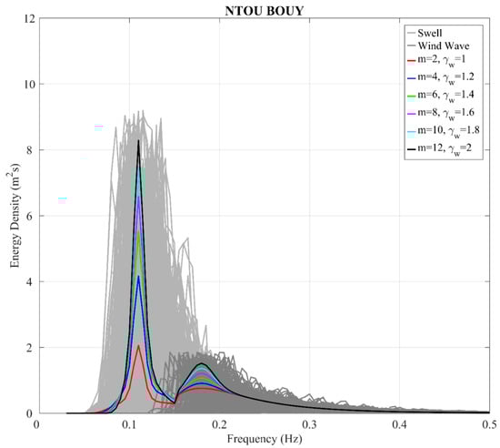
Figure 14.
The JW-J spectra corresponding to different m and γω values for Hs = 1.0 m, Tsp = 10 s, and Twp = 5.6 s.
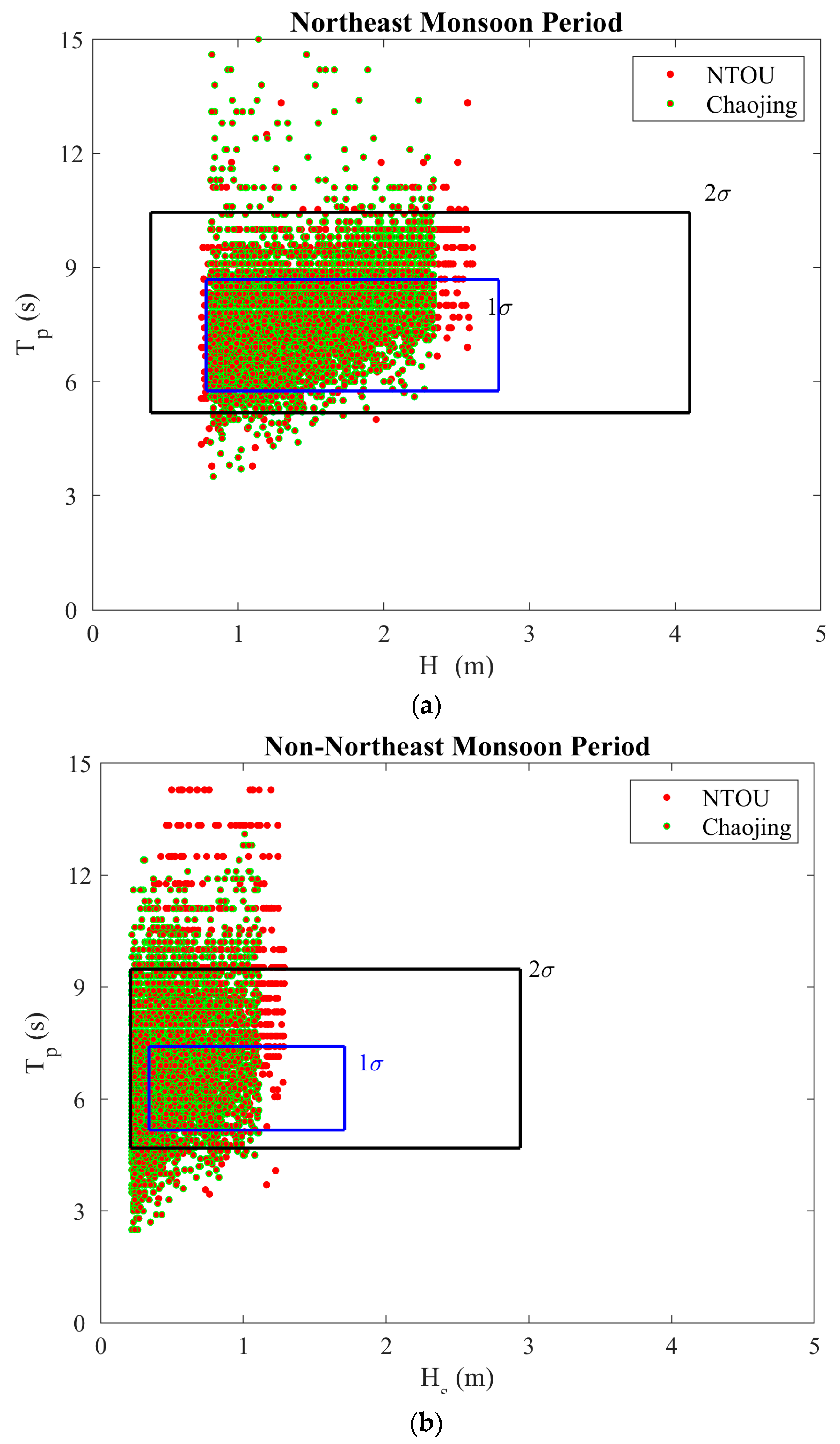
On the other hand, we also attempted to discuss whether Hs and Tp in this region are similar. In the future, when studying locations near this area without buoy data, it could be possible to use results from nearby known stations as an evaluation basis. Therefore, we collected data on Hs and Tp from the nearby Chaojing station (location is 25°8′37″ N, 121°48′29.5″ E, and the water depth is 25 m) and plotted it with the data from the NTOU station in Figure 15.

Figure 15.
Application of parameter data from Pengjia Islet and Fugui Cape stations to NTOU buoy and Chaojing station during (a) the northeast and (b) non-northeast monsoon periods.
In Figure 15a, during the northeast monsoon period, it can be observed that the data from the two stations exhibit high similarity. The blue line area represents the range defined by one standard deviation for the Pengjia Islet and Fugui Cape stations, and most of the data points fall within this range. Expanding the range to two standard deviations (black line area) covers almost all data points, with only a few scattered outside the range. This indicates that during the northeast monsoon period, the variations in Hs and Tp are relatively small, and that assessment can be made using data from nearby stations.
Figure 15b presents the results for the non-northeast monsoon period. The figure shows that only about 1/3 of the data points are included within the one standard deviation range. Most data points are covered when expanding to the two standard deviation range. However, many data points are scattered outside the range compared to the northeast monsoon period. This suggests that waves may be more influenced by faraway swell systems rather than just the local wind field during non-northeast monsoon periods and is worth further in-depth research in the future.
5. Conclusions
This study collected unidimensional wave spectrum data measured in the waters off the northeast coast of Taiwan. Different unimodal and bimodal wave spectrum models were used to fit and analyze the measured data, and some notable findings are summarized as follows:
- In terms of spectral types
- a.
- In this region, whether during the northeast or non-northeast monsoon periods, the proportion of single-peak spectra is deficient, not exceeding 0.5%. During the northeast monsoon, the proportion of dual-peak spectra can exceed 80%, while the proportion of unimodal spectra is between 8–15%. During non-northeast monsoon periods, the proportion of unimodal spectra increases, reaching 30–50%, while the proportion of dual-peak spectra decreases.
- b.
- Wind waves dominate both at the Pengjia Islet and Fugui Cape stations, whether during the northeast or non-northeast monsoon periods, accounting for 60–80%. Swell and jointly dominant wave systems represent 10–20% and less than 15%, respectively. However, swell dominates at the Ocean University wave buoy station, with the highest proportion exceeding 80%.
- In terms of spectral fitting models
- a.
- Concerning unimodal spectra, at the Pengjia Islet station, the JONSWAP spectrum has the best fitting performance, accounting for 43.75%. It may be due to the proximity of this area to the open sea. At the Fugui Cape station, the TMA spectrum exhibits the optimal fitting performance, representing 31.5%. This could be attributed to the closer proximity to the nearshore, and the TMA spectrum is more suitable for limited water depth conditions. Due to the lack of unimodal spectrum data for the NTOU wave buoy station, related analyses could not be conducted.
- b.
- In the case of bimodal spectra, a new bimodal spectrum model was proposed in this study, combining the JW and JONSWAP spectra to describe swell and wind wave systems, respectively. At the Pengjia Islet station, the optimal spectrum model is the OH spectrum, accounting for 65.87%, while the proposed JW-J spectrum accounts for 27.16%. At the Fugui Cape station, the OH spectrum achieves the highest fitting performance at 49.58%, but the proposed JW-J spectrum also reaches 46.48%. At the NTOU wave buoy station, similar to the Fugui Cape station, the OH spectrum and JW-J spectrum have fitting performances of 51.24% and 42.70%, respectively. The most optimal spectral fitting models of unimodal and bimodal spectra are discussed in this study. However, as indicated in our research, approximately 30–50% of the spectra in this region are unformed during non-northeast monsoon periods. This aspect could be further explored to determine which spectral model is more appropriate for fitting, providing a more comprehensive understanding of the wave characteristics in this area.
- c.
- This study also analyzed and discussed the wave characteristic parameters of the JW-J spectrum, finding that the spectral parameters influencing its fitting are the shape parameter m and the spectral peak enhancement factor γw. At the Pengjia Islet station, the ranges for m and γw are 4.20 to 12.72 and 0.02 to 0.86, respectively. At the Fugui Cape station, m and γw range from 5.10 to 13.85 and 0.04 to 1.90, respectively.
- d.
- Applying the analyzed results of the JW-J spectrum characteristic parameters from the Pengjia Islet and Fugui Cape stations to the NTOU wave buoy station, assuming an Hs of 1.0 m, Tp for swell and wind waves of 10 s and 5.6 s, and setting m and γw to 12 and 2, the spectrum results can roughly encompass the measured results at the NTOU wave buoy. On the other hand, we also examined whether this region has a similar range of Hs and Tp. Therefore, observational data from a nearby Chaojing station were analyzed. It was found that during the northeast monsoon period, the data were roughly covered within one standard deviation, and when expanded to two standard deviations, almost all data points were covered. However, only about 1/3 of the data points were covered within one standard deviation during the non-northeast monsoon period. Over 80% of data points were covered when the area expanded to two standard deviations. In the future, it is worth further in-depth research to determine the respective proportions of wind and swells at neighboring stations during the same time. This analysis is essential for understanding the differences in the impact of distant weather systems on nearby stations. Through such an analysis, we can further adjust and optimize the spectral parameters to better suit the local conditions.
Author Contributions
Conceptualization, W.-T.C., T.-C.L. and T.-W.H.; methodology, W.-T.C., T.-C.L. and K.-C.H.; validation, W.-T.C. and T.-C.L.; formal analysis, W.-T.C.; investigation, W.-T.C., T.-C.L. and T.-W.H.; resources, T.-W.H.; writing—original draft preparation, W.-T.C. and T.-C.L.; writing—review and editing, W.-T.C. and T.-C.L.; visualization, W.-T.C., T.-C.L. and K.-C.H.; supervision, T.-C.L. and T.-W.H.; project administration, T.-W.H.; funding acquisition, T.-W.H. All authors have read and agreed to the published version of the manuscript.
Funding
This research was funded by the National Science and Technology Council, Taiwan grant number NSTC 112-2218-E-019-001-.
Institutional Review Board Statement
Not applicable.
Informed Consent Statement
Not applicable.
Data Availability Statement
Data are contained within the article.
Acknowledgments
The authors thank the anonymous reviewers for their insightful and constructive comments to improve this paper. This study was provided by the National Science and Technology Council (NSTC) of the Ministry of Education, Taiwan. The observation data used in this study were measured and provided by the Central Weather Bureau of Taiwan. The authors would like to express great thanks for all the support.
Conflicts of Interest
The authors declare no conflict of interest.
References
- Lee, U.J.; Jeong, W.M.; Cho, H.Y. Estimation and analysis of JONSWAP spectrum parameter using observed data around Korean Coast. J. Mar. Sci. Eng. 2022, 10, 578. [Google Scholar] [CrossRef]
- Lee, H.S.; Kim, S.D. A comparison of several wave spectra for the random wave diffraction by a semi-infinite breakwater. Ocean Eng. 2006, 33, 1954–1971. [Google Scholar] [CrossRef]
- Ochi, M.K. Ocean Waves: The Stochastic Approach; Cambridge University Press: Cambridge, UK, 2005; p. 332. [Google Scholar]
- Massel, S.R. Ocean Surface Waves: Their Physics and Prediction, 3rd ed.; World Scientific: Singapore, 2017; p. 800. [Google Scholar]
- Shukla, J.B.; Arora, M.S.; Verma, M.; Misra, A.K.; Takeuchi, Y. The impact of sea level rise due to global warming on the coastal population dynamics: A modeling study. Earth Syst. Environ. 2021, 5, 909–926. [Google Scholar] [CrossRef]
- Valipour, M.; Bateni, S.; Jun, C. Global surface temperature: A new insight. Climate 2021, 9, 81. [Google Scholar] [CrossRef]
- Pierson, W.J. A Unified Mathematically Theory for the Analysis Propagation and Refraction of Storm Generated Ocean Surface Waves. Part I and II; New York University: New York, NY, USA, 1952. [Google Scholar]
- Neumann, G. On ocean wave spectra and a new method of forecasting wind generated sea. Beach Erosion Board Tech. Memo. 1953, 43, 46. [Google Scholar]
- Pierson, W.J.; Moskowitz, L. A proposed spectral form for fully developed wind seas based on the similarity theory of S. A. Kitaigorodskii. J. Geophys. Res. 1964, 69, 5181–5190. [Google Scholar] [CrossRef]
- Bretschneider, C.L. Significant waves and wave spectrum. In Ocean Industry; Gulf Publishing Company: Houston, TX, USA, 1968; pp. 40–46. [Google Scholar]
- Mitsuyasu, H. On the Growth of Wind-Generated Waves (2)—Spectral Shape of Wind Waves at Finite Fetch. In Proceedings of the 17th Japanese Conference, Kyoto, Japan, 16–21 October 1970. [Google Scholar]
- Hasselmann, K.; Barnett, T.P.; Bouws, E.; Carlson, H.; Cartwright, D.E.; Enke, K.; Ewing, J.A.; Gienapp, A.; Hasselmann, D.E.; Kruseman, P.; et al. Measurements of wind-wave growth and swell decay during the Joint North Sea Wave Project (JONSWAP). Dtsch. Hydrogr. Z. 1973, 8, 1–95. [Google Scholar]
- Bouws, E.; Günther, H.; Rosenthal, W.; Vicent, C.L. Similarity of the wind wave spectrum in finite depth water 1. Spectral form. J. Geophys. Res. 1985, 90, 975–986. [Google Scholar] [CrossRef]
- Phillips, O.M. The equilibrium range in the spectrum of wind-generated waves. J. Fluid Mech. 1958, 4, 426–434. [Google Scholar] [CrossRef]
- Toba, Y. The 3/2-power law for ocean waves and its applications. In Advances in Coastal and Ocean Engineering; World Scientific: Singapore, 1997; pp. 31–65. [Google Scholar]
- Battjes, J.A.; Zitman, T.J.; Holthuusen, L.H. A reanalysis of the spectra observed in JONSWAP. J. Geophys. Res. 1987, 17, 1288–1295. [Google Scholar] [CrossRef]
- Liu, P.C. On the slope of the equilibrium range in the frequency spectrum of wind waves. J. Geophys. Res. 1989, 94, 5017–5023. [Google Scholar] [CrossRef]
- Kitaigorodskii, S.A.; Krasitskii, V.P.; Zaslavskii, M.M. On Phillips Theory of equilibrium range in the spectra of wind-generated gravity waves. J. Phys. Oceanogr. 1975, 13, 816–827. [Google Scholar] [CrossRef]
- Huang, N.E.; Long, S.R.; Tung, C.C.; Yuen, Y.; Bliven, L.F. A unified two-parameter wave spectral model for a general sea state. J. Fluid Mech. 1981, 112, 203–224. [Google Scholar] [CrossRef]
- Gao, X.; Ma, X.; Huang, X.; Zheng, Z.; Dong, G. Spectral characteristics of swell-dominated seas with in situ in the coastal seas of Peru and Sri Lanka. J. Atmos. Ocean. Technol. 2022, 39, 755–770. [Google Scholar] [CrossRef]
- Goda, Y. Analysis of wave grouping and spectra of long travelled swell. Rep. Port Harb. Res. Inst. Rep. 1983, 22, 3–41. [Google Scholar]
- Olagnon, M.; Ewans, K.; Forristall, G.; Prevosto, M. West Africa swell spectral shapes. In Proceedings of the ASME 2013 32nd International Conference on Ocean, Offshore and Arctic Engineering, Nantes, France, 9–14 June 2013. [Google Scholar]
- Lucas, C.; Guedes Soares, C. On the modelling of swell spectra. Ocean Eng. 2015, 108, 749–759. [Google Scholar] [CrossRef]
- Guedes Soares, C. Representation of double-peaked sea wave spectra. Ocean Eng. 1984, 11, 185–207. [Google Scholar] [CrossRef]
- Freilich, M.H.; Guza, R.T. Nonlinear Effects on Shoaling Surface Gravity Waves. Philos. Trans. R. Soc. London Ser. A Math. Phys. Sci. 1984, 311, 1–41. [Google Scholar]
- Strekalov, S.; Massel, S. On the spectral analysis of wind waves. Arch. Hydrol. 1971, 18, 457–485. [Google Scholar]
- Akbari, H.; Panahi, R.; Amani, L. A double-peaked spectrum for the northern parts of the Gulf of Oman: Revisiting extensive field measurement data by new calibration methods. Ocean Eng. 2019, 180, 187–198. [Google Scholar] [CrossRef]
- Ewans, K.C.; Bitner-Gregersen, E.M.; Soares, C.G. Estimation of wind-sea and swell components in a bimodal sea state. J. Offshore Mech. Arct. Eng. 2006, 128, 265–270. [Google Scholar] [CrossRef]
- Torsethaugen, K. A two peak wave spectrum model. In Proceedings of the 12th International Conference on Offshore Mechanics and Arctic Engineering, Glasgow, UK, 20–24 June 1993; pp. 175–180. [Google Scholar]
- Torsethaugen, K. Simplified double peak spectral model for ocean waves. In Proceedings of the 41st Design Automation Conference, San Diego, CA, USA, 7–11 June 2004. [Google Scholar]
- Akbari, H.; Panahi, R.; Amani, L. Improvement of double-peaked spectra: Revisiting the combination of the Gaussian and the JONSWAP models. Ocean Eng. 2020, 198, 106965. [Google Scholar] [CrossRef]
- Ochi, M.K.; Hubble, E.N. Six-parameter wave spectra. Coast. Eng. Proc. 1976, 1, 17. [Google Scholar] [CrossRef]
- Golpira, A.; Panahi, R.; Shafieefar, M. Developing families of Ochi-Hubble spectra for the northern parts of the Gulf of Oman. Ocean Eng. 2019, 178, 345–356. [Google Scholar] [CrossRef]
- Panahi, R.; Shafieefar, M.; Ghasemi, A. A new method for calibration of unidirectional double-peak spectra. J. Mar. Sci. Technol. 2016, 21, 167–178. [Google Scholar] [CrossRef]
- Mazaher, S.; Imani, H. Evaluation and modification of JONSWAP spectral parameters in the Persian Gulf considering offshore wave characteristics under storm conditions. Ocean Dyn. 2019, 69, 615–639. [Google Scholar] [CrossRef]
- Toffoil, A.; Onorato, M.; Monbaliu, J. Wave statistics in unimodal and bimodal seas from a second-order model. Eur. J. Mech. B Fluids 2006, 25, 649–661. [Google Scholar] [CrossRef]
- Orimoloye, S.; Karunarathna, H.; Reeve, D.E. Effects of Swell on Wave Height Distribution of Energy-Conserved Bimodal Seas. J. Mar. Sci. Eng. 2019, 7, 79. [Google Scholar] [CrossRef]
- Benassai, G.; Motuori, A.; Nunziata, F. Sea wave modeling with X-band COSMO-SkyMed SAR-derived wind field forcing and applications in coastal vulnerability assement. Ocean Sci. 2013, 9, 325–341. [Google Scholar] [CrossRef]
- Orimoloye, S.; Horrillo-Caraballo, J.M.; Karunarathna, H.; Reeve, D.E. Wave overtopping of smooth impermeable seawalls under Unidirectional Bimodal Sea Conditions. Coast. Eng. 2020, 165, 103792. [Google Scholar] [CrossRef]
- Chiu, F.C.; Huang, W.Y.; Tiao, W.C. The spatial and temporal characteristics of the wave energy resources around Taiwan. Renew. Energy 2013, 52, 218–221. [Google Scholar] [CrossRef]
- Gilhousen, D.B.; Hervey, R. Improved estimates of swell from moored buoys. In Processing of the Fourth International Symposium Waves 2001; ASCE: Alexandria, VA, USA, 2001; pp. 387–393. [Google Scholar]
- Rodríguez, G.; Guedes Soares, C. The Bivariate Distribution of Wave Heights and Periods in Mixed Sea States. J. Offshore Mech. Arct. Eng. 1999, 121, 102. [Google Scholar] [CrossRef]
- Kitaigorodskii, S.A. Application of the theory of similarity to the analysis of wind-generated wave motion as a stochastic process. Izv. Akad. Nauk. SSSR Ser. Geophys. 1962, 1, 105–117. [Google Scholar]


Disclaimer/Publisher’s Note: The statements, opinions and data contained in all publications are solely those of the individual author(s) and contributor(s) and not of MDPI and/or the editor(s). MDPI and/or the editor(s) disclaim responsibility for any injury to people or property resulting from any ideas, methods, instructions or products referred to in the content. |
© 2023 by the authors. Licensee MDPI, Basel, Switzerland. This article is an open access article distributed under the terms and conditions of the Creative Commons Attribution (CC BY) license (https://creativecommons.org/licenses/by/4.0/).