An Adaptive Control Strategy for Underwater Wireless Charging System Output Power with an Arc-Shaped Magnetic Core Structure

Abstract

Aiming at the problem of unstable output power of wireless charging systems for autonomous underwater vehicles (AUVs), a magnetic coupler (MC) with an arc-shaped core structure is introduced and an output power stabilization control strategy based on mutual inductance identification algorithm is proposed. Firstly, an arc-shaped MC with high tolerances, excellent magnetic coupling and weak electromagnetic interference (EMI) is designed for the cylinder-shaped AUV. Based on ANSYS Maxwell simulation, an analysis of the magnetic field and comparative misalignment tests are carried out for the arc-shaped and the double dipole core structures. Secondly, a mathematical model of the LCC-S type magnetically coupled resonant wireless power transfer (MCR-WPT) system is developed, and a particle swarm parameter identification algorithm with adaptive inertia weights is proposed. Finally, the output power is steadily controlled by real-time adaptation of the duty cycle for the Buck-Boost circuit. The results show there is a maximum error within 2.5% in mutual inductance identification when the load is changed from 0 Ω to 12 Ω and the mutual inductance is changed from 25 μH to 50 μH. The system output power is steady at around 680 W with a maximum fluctuation rate of 4.90%, which verifies the efficiency of the power stabilization control strategy.

1. Introduction

The ocean contains enormous resources, including mineral resources such as combustible ice, oil and gas, and economic resources such as aquaculture, fishing and tourism [1]. With the advancement of marine navigation technology and the implementation of renewable energy strategies, it is becoming increasingly common for underwater marine resources to be exploited. Autonomous Underwater Vehicles (AUVs) play an important role in water quality detection, information interact-ion, seafloor mapping and mineral resource exploration [2]. There are two main ways of supplying energy to the AUV. One way is for the battery to be recharged at the nearest charging station when it is about to be exhausted, which is time-consuming and non-confidential. Another way is to recharge the AUV by cable from the mother ship, which lacks security and requires high docking accuracy [3].

Wireless Power Transfer (WPT) is being developed and promoted due to its obvious advantages in environmental friendliness, convenience, safety and applicability. Unlike wireless charging technology on land, the ocean is full of turbulent currents and complex environments. During the charging of the AUV, the impact of the water flow will cause varying degrees of jitter, which will lead to a change in the relative position of the transmitting side to the receiving side of the AUV. These changes not only bring about fluctuations in the reflected impedance and drift in the operating frequency, but also reduce the transmitted power and efficiency [4,5]. When the reflected impedance and mutual inductance change, the system requires real-time adjustment the control strategy to ensure the performance indicators such as system stability and efficiency [6].

Currently, the main measures to improve the transmission capacity and stability of the system are as follows: design of proper compensation circuits, optimum magnetic coupler (MC), controlled coordinately with multi-pole coils and increase the power control circuit [7,8]. The WPT system’s output capacity and transmission efficiency are primarily determined by the MC, which is the system’s fundamental component. Feezor et al. designed an AUV underwater wireless charging system with a transmission power of 200 W [9]. Kojiya et al. designed a conical coil core structure that achieved a transmission power of 500 W and a transmission efficiency of 96% [10]. Chen et al. built an AUV charging system with 450 W power, efficiency more than 85% and voltage stability 7% with a can-shaped MC [11]. Kan et al. segmented the secondary side toroidal MC and used the I-shaped cores on the primary side, which had the advantages of lightweight mass and high tolerances [12]. Lee et al. improved the anti-angle offset performance of the system with a modular diode coil based on flooding the Wi power region with DQTx modules [13].

In addition, power control technology is essential for the stability of the system’s output power. The WPT power control methods are mainly classified as primary side control, secondary side control and bilateral side control. All three control methods regulate and control the system by adding additional telecommunication devices, various power electronic converters and closed loop control on different sides of the system [14,15,16]. It is essential for power control technology to obtain real-time and efficient information on parameters such as the load and the mutual inductance. Currently, research is being carried out on the load and mutual sense identification technologies for MCR-WPT systems by relevant universities and research institutes [17,18,19,20,21]. By identifying the operating frequency, inverter output voltage, and current rms values of the S/P type MC-WPT system in the frequency domain, Reference [17] adopted the fundamental wave approximation principle to calculate the load and mutual inductance values. The maximum identification error of the load and mutual inductance values was approximately 5.50% and 4.42%. By changing the frequency of the SS-type MCR-WPT system at the non-operating frequency point, Reference [18] was able to identify the load and mutual inductance, and the experimental identification result error was less than 3%. By including a series of auxiliary inverters and matching MC on the transmitter side of the SS-type MCR-WPT system, which functioned in various modes, Reference [19] completed the identification of load and mutual inductance. Reference [20] proposed a swarm optimisation algorithm and genetic algorithm for inductor–capacitor–capacitor series (LCC-S) systems under phase-shift control, which enables inductor and load identification at any phase-shift angle by configuring a series genetic particle swarm optimisation (GA-PSO) algorithm. Chow et al. evaluated mutual inductance by utilizing a time-domain mathematical model of the electrical information on the transmitting side [21]. In summary, the main problems with traditional load and mutual sense identification methods for MCR-WPT systems are as follows.

(1)

Most of the studies and analyses are on SS type compensation circuits, other topologies were rarely studied.

(2)

Some recognition algorithms have low accuracy and long recognition times.

(3)

Part of the identification method requires multiple switching of the system operating frequency and additional auxiliary mechanisms, which increases the complexity of the system.

(4)

There is not an in-depth study that takes into account mutual inductance and load detection, including efficient closed-loop control, performance analysis, etc.

This paper is organized as follows. Section 2 introduces an arc-shaped MC for cylindrical AUVs, and then uses finite element software to analysis the MC performance. Section 3 introduces the mathematical modelling of the LCC-S type MCR-WPT system. Section 4 introduces an inertial weighted adaptive particle swarm identification technique with asymmetric learning factors for detecting time-varying coupler mutual inductance. In Section 5, it is suggested that the duty cycle of the Buck-Boost circuit be changed in real time to ensure steady management of the required power. Finally, Section 6 concludes the whole paper.

2. Optimization of the MC

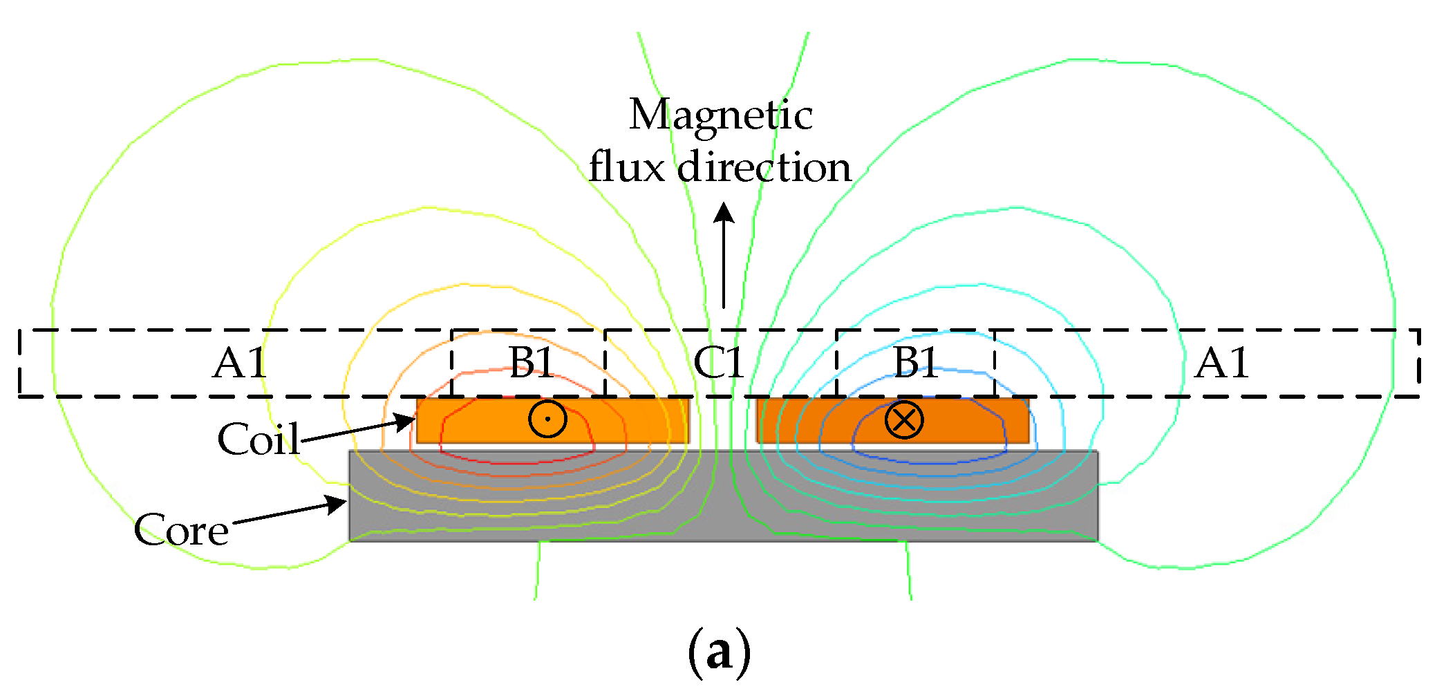
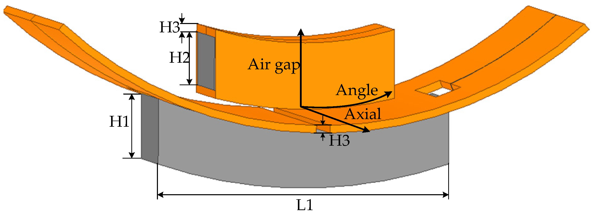
2.1. Analysis and Design of the Proposed MC

The following are the five most popular MC configurations: conical, can-shaped, ε-shaped, ring-shaped and segmented ring-shaped. The conical, can-shaped MCs are generally larger and heavier in mass, which increases the resistance of the AUV when sailing. It is also extremely demanding on the docking and positioning devices of the AUV, which can cause some interference with navigation systems such as sonar. The ε-shaped is less resistant to angle offset than the E-shaped magnets, although it reduces the gap between the core and the housing. The ring-shaped core is more resistant to angle offset, but magnetic field measurement reveals that it has a significant magnetic leakage and has a significant impact on the electromagnetic interference (EMI) of the electronics and other precision equipment inside the AUV. The segmented ring-shaped core, which is created for a ring-shaped core, successfully eliminates magnetic leakage, but the issue of excessive core weight overall is still present. In summary, the design of the MC should take into account factors such as size, quality and EMI with the internal electronics while improving the resistance to misalignment.

According to the magnetic field characteristics of the primary-side emitting core, the MC can be divided into three categories: unipolar, bipolar and array type, where the array type is a combination of the first two. The magnetic field distribution for planar unipolar and bipolar is shown in Figure 1. The lines in the figure are magnetic lines of force and the thickness of the lines represents the strength of the magnetic field here. From the analysis of the magnetic field simulation results, it can be seen that the effective magnetic field area on the receiving side of the bipolar emission field (C2 region) is significantly larger than that on the receiving side of the unipolar emission field (B2 region) with the same size core structure. The magnetic field strength analysis shows that the leakage flux in the A1 region of a unipolar emitting magnetic field is greater than that in the A2 region of a bipolar emitting magnetic field. In summary, in comparison to unipolar emitting fields, bipolar emitting fields have obvious advantages with the misalignment sensitivity, magnetic coupling capability and low leakage flux.

A typical cylindrical AUV structure and docking system, as shown in Figure 2. The AUV diameter is 300 mm and the enclosure thickness is 4 mm. The instrumentation and main propulsion bins have been fitted with numerous sophisticated sensors and electronics, as shown in Figure 2. It can be seen that there is still a tiny rounded space inside the pressurized lithium battery pack and yellow housing of the battery compartment. Therefore, the planar bipolar structure was changed to a circular structure that fits closely to the outer wall of the AUV to reduce the air gap as much as possible.

In terms of magnetic energy utilization, the scheme with parallel sides of the core is more effective than the scheme with perpendicular circular tangents of the core [22]. Therefore, the core structures in this paper use a parallel scheme on both sides of the core. The MC with an arc-shaped structure on the secondary side has been designed combining the excellent magnetic chain collecting ability of the double dipole structure. The arc-shaped core and the double dipole core structure are shown in Figure 3a,b respectively [23]. Compared to the designed arc-shaped core structure, the double-dipole MC has an arc on the secondary side which is the same arc length as the primary side. The two coils on the primary side are tightly wound using a single copper wire and ensuring that the coils are wound in opposite directions on both sides in order to form an effective magnetic circuit. The coils on the secondary side are wound tightly in the vertical direction of the secondary core according to the right-hand spiral rule. The parameters of the arc core structure are shown in

Table 1. Parameters of the MC.

Symbol	Parameters	Value
W1	Primary winding line width	50 mm
G1	Primary coil and core gap	2°
W2	Primary core width	48 mm
G2	Primary coil 1, 2 gap	1°
H1	Primary core height	24 mm
L1	Primary core length	114 mm
H2	Secondary core height	20 mm
L2	Secondary core length	71 mm
W3	Secondary core width	48 mm
H3	Height of primary coil 1, 2, 3	0.3 mm
N1, N2	Primary coil turns	17 turns
N3	Secondary coil turns	19 turns

(the parameters are labelled in Figure 3a and Figure 4).

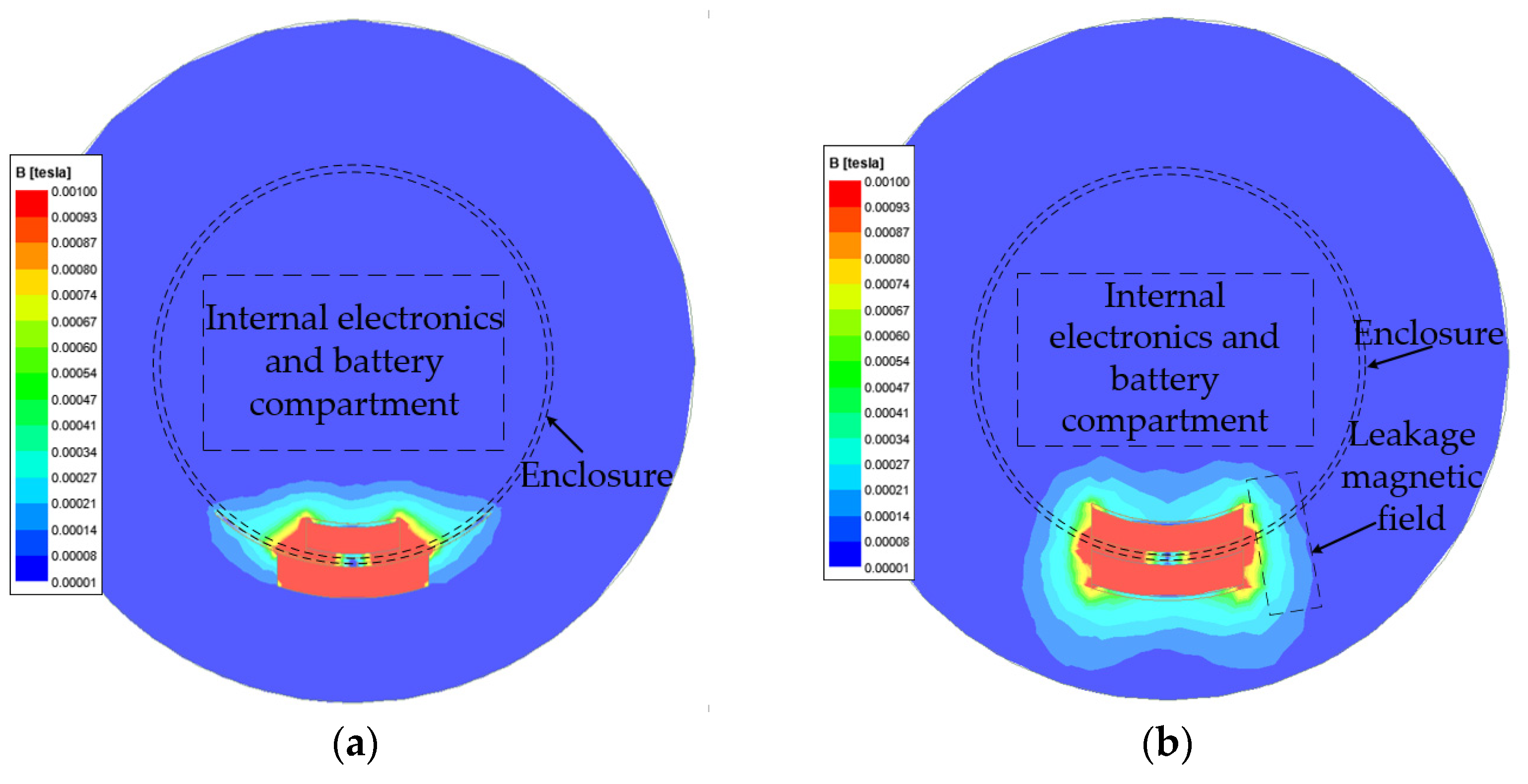
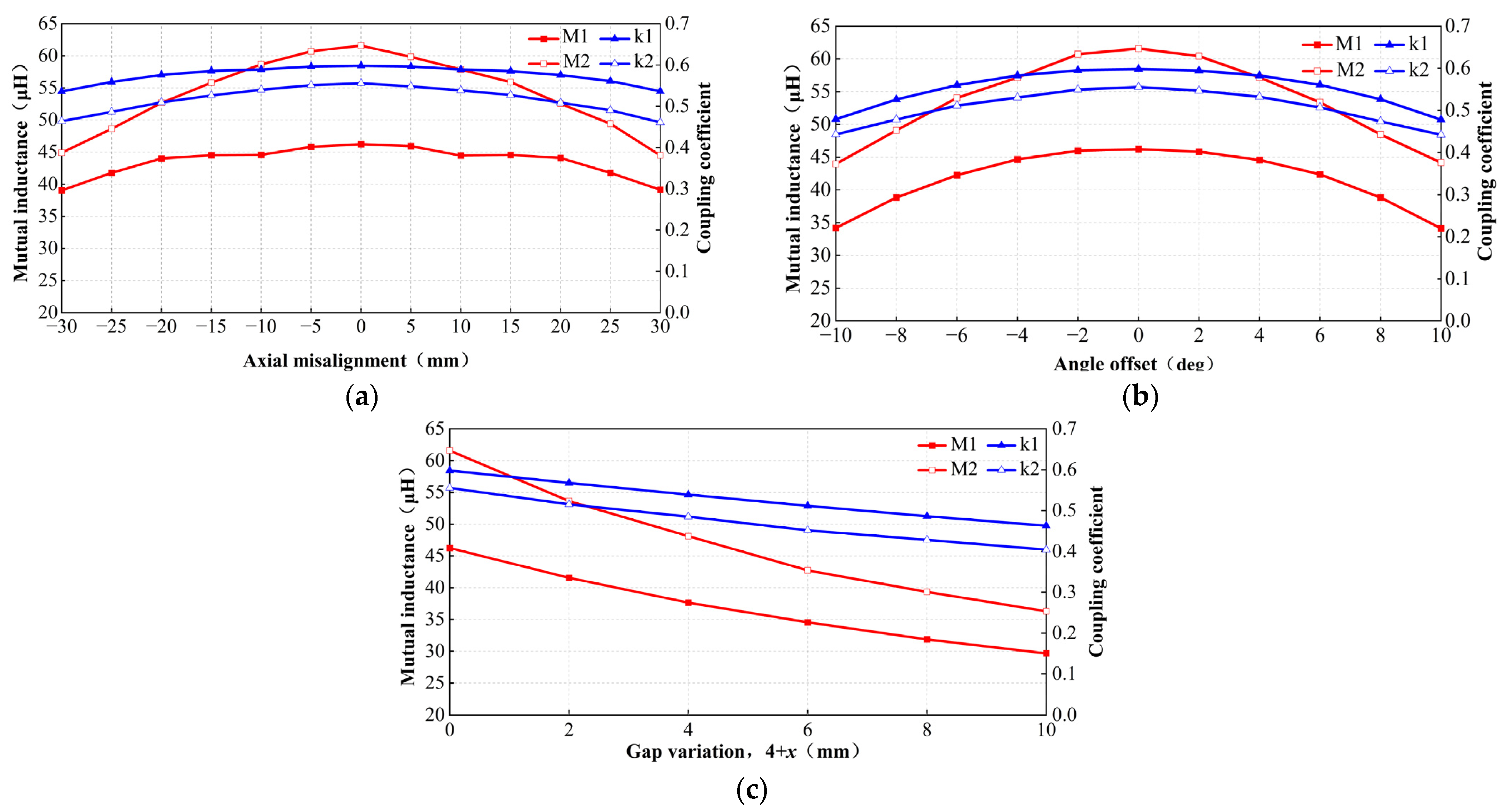
2.2. Performance Analysis and Misalignment Experiments

Using ANSYS Maxwell software to model and analysis the two core structures, the static magnetic field distribution is shown in Figure 5. The figure shows that the magnetic inductance of both the arc-shaped core and the double dipole core structures are concentrated on the core, confirming the excellent magnetic transfer capability of both structures. The arc-shaped core structure has a lower magnetic induction strength inside the AUV than the double dipole core, which indicates less electromagnetic interference (EMI) with the AUV’s electronics. In addition, the double dipole core structure has obviously larger leakage fields around the core than the arc-shaped core structure, which has a greater impact on the transmission efficiency and electromagnetic shielding of the entire coupler.

Furthermore, it is necessary to test the coupling performance of the MC by performing misalignment experiments in three dimensions The three directions of misalignment are axial misalignment, angle offset and gap variation, the specific directions are marked in Figure 4. Set the axial misalignment of ±30 mm, the angle offset of ±10°, and the gap variation range of 0 mm to 10 mm. Comparison experiments on the misalignment of the designed arc-shaped core structure and the double dipole core structure respectively. Record the results of the experiment, as shown in Figure 6 (1 represents the arc-shaped core structure, 2 represents the double dipole core structure).

According to the misalignment results in Figure 6, with axial misalignment of 0 mm and gap of 4 mm, the mutual inductance and coupling coefficients are 46.240 μH and 0.598 and 61.579 μH and 0.555 for the arc-shaped core structure and the double dipole core structure, respectively. Setting the angle offset at 0° and gap at 4 mm, the axial misalignment test changes from −30 mm to 30 mm at 5 mm intervals uniformly and the mutual inductance and coupling coefficients decrease by 7.207 μH and 0.062, 17.095 μH and 0.094 for the arc-shaped core structure and the double dipole core structure, respectively. Setting axial misalignment at 0 mm and gap of 4 mm, the angle offset test changes from −10° to 10° every 2 degrees uniformly, and the mutual inductance and coupling coefficients decrease by 12.115 μH and 0.120, 17.615 μH and 0.113, respectively. Setting axial misalignment at 0 mm and angle offset at 0°, the gap variation test changes uniformly from 4 mm to 14 mm every 2 mm, and the mutual inductance and coupling coefficients decrease by 16.571 μH and 0.135, 25.288 μH and 0.151 for the arc-shaped core structure and double dipole core structure, respectively.

From the misalignment simulation results, it can be seen that the arc-shaped core structure and double dipole core structure show excellent stability in axial misalignment, but they are more sensitive to changes in gap and angle. The auxiliary clamping device is designed for this deficiency, as shown in Figure 7. When the navigator is not in the docking system, the primary side of the coupler is retracted in the hidden slot. When the signal for clamping is received from the positioning structure, a push rod starts to extend the primary side core, which is at 90° to each other, to the set position.

3. System Introduction and Mathematical Modeling

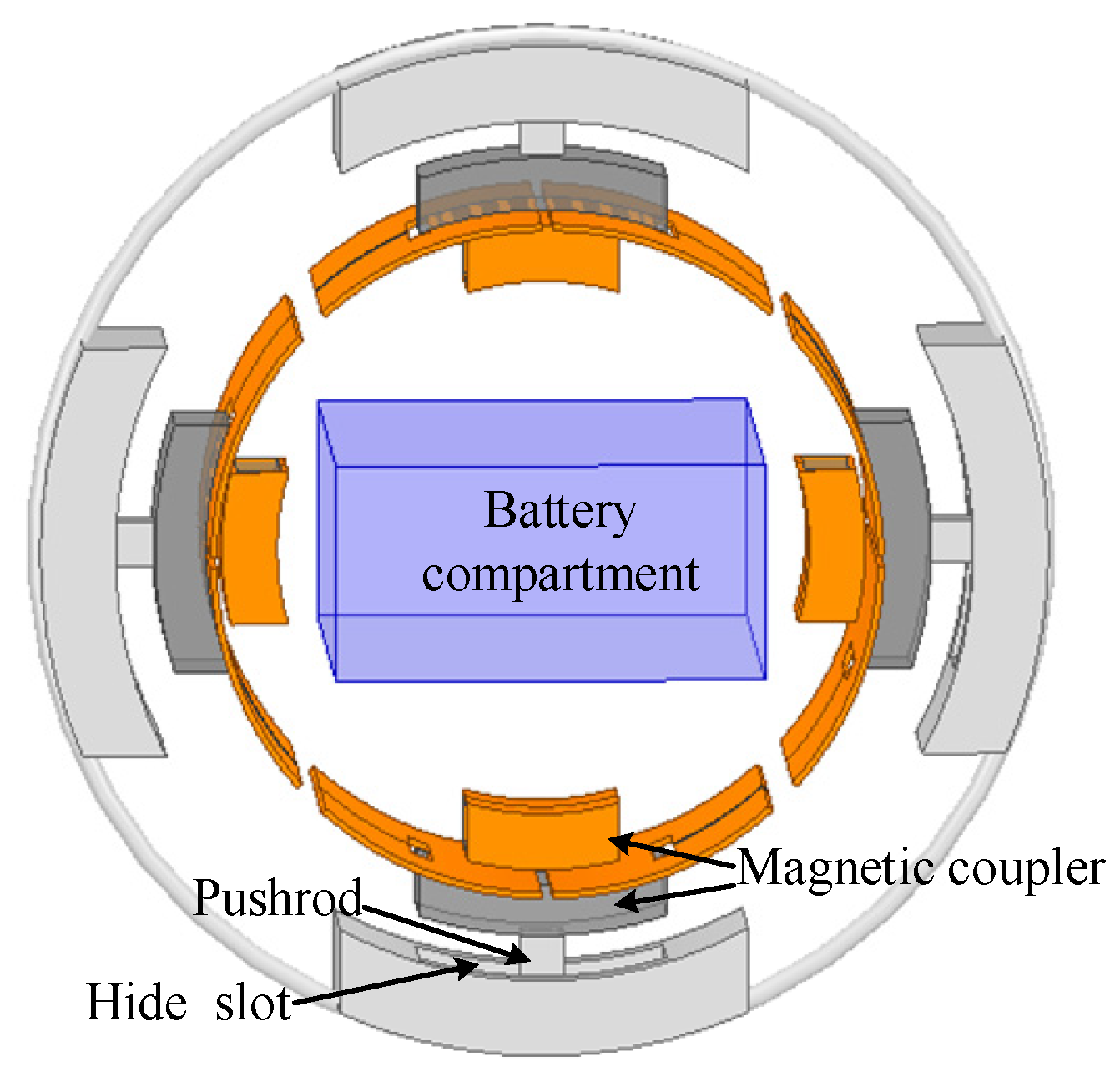
3.1. System Overview

With a symmetrical T-compensation topology circuit on the primary side, the LCC-S type MCR-WPT system is insensitive to changes in the system’s power electronics parameters. It is possible to set the circuit settings to balance the voltage and current stress on the components, match the “optimum impedance,” and maintain a constant current in the primary coil. Therefore, the example of the LCC-S type MCR-WPT circuit is analyzed in this paper [24].

The LCC-S circuit topology is shown in Figure 8. E_dc is the DC source, r is the internal resistance of the DC source, S1~S2 are the main body of the high-frequency inverter circuit composed of four MOSFET, U_f is the output voltage of the inverter bridge, I_f is the output current of the inverter bridge, C_f and C₁ are the primary side parallel and series compensation capacitors, respectively. L_f is the primary series compensation inductance, L₁ and L₂ are the inductances of the primary and secondary resonant coils, respectively. M is the mutual inductance of the magnetic coupler, R₁ and R₂ are the equivalent resistance of the primary and secondary resonant coils. I₁ and I₂ are the current flowing through the primary and secondary coils, respectively. C₂ is the secondary side series compensation capacitor. D₁ to D₄ form the main body of the rectifier circuit. C is the rectifier filter capacitor. S, L_d and C_d constitute the main part of the Buck-Boost circuit. R_L is the equivalent resistance of the AUV and U_L is the voltage across the load.

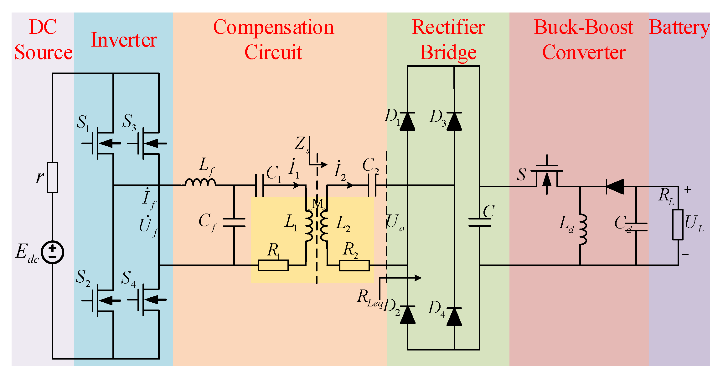
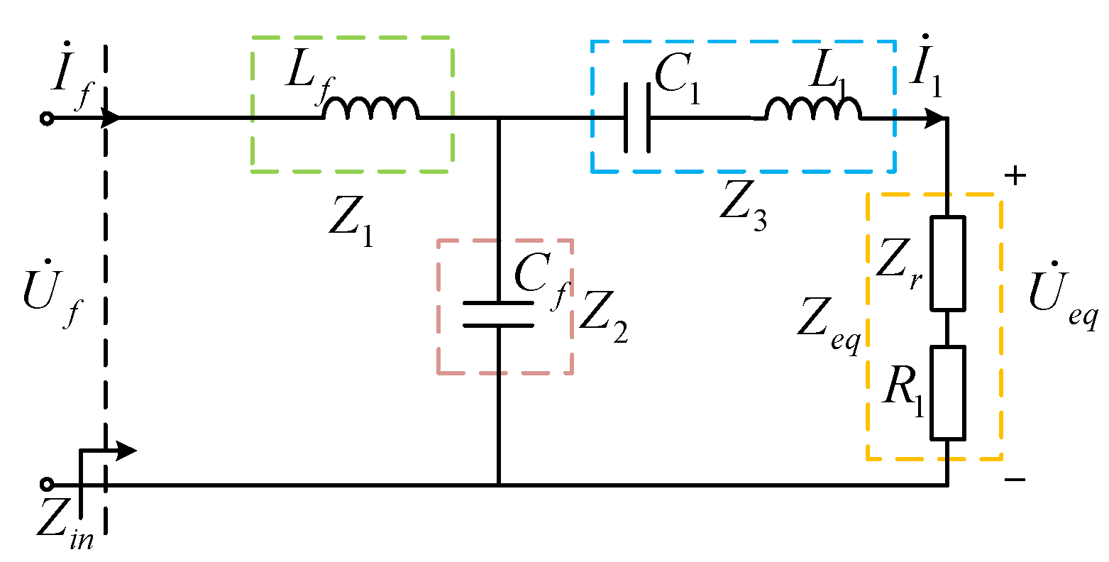
3.2. Mathematical Modeling of LCC-S System

According to the relevant literature, the equivalent resistance R_Leq formed by the rectifier bridge, Buck-Boost circuit and load R_L satisfies [25]:

$$R_{Leq}=\frac{8{(1-\alpha )}^2}{{\pi }^2{\alpha }^2}{R}_L.$$

(1)

where α is the duty cycle of the Buck-Boost circuit, the equivalent impedance of the secondary circuit Z_s is

$$Z_s=R_2+R_{Leq}+j\omega L_2+\frac{1}{j\omega C_2}.$$

(2)

The secondary side circuit is converted to the primary side, and the DC power supply is equivalent. In order to facilitate the derivation of the mathematical model, the internal resistance r of the power supply is ignored, and the equivalent circuit is shown in Figure 9.

The reflected resistance of the secondary circuit equivalent impedance Z_s converted to the primary side is Z_r.

$$Z_r=\frac{{\omega }^2{M}^2}{Z_s}$$

(3)

Mathematical modeling based on knowledge of two-port networks shows that

$$\left[\begin{array}{c}{\dot{U}}_f\\ {\dot{I}}_f\end{array}\right]=\left[\begin{array}{cc}{A}_{11}& A_{12}\\ A_{21}& A_{22}\end{array}\right]\cdot \left[\begin{array}{c}{\dot{U}}_{eq}\\ {\dot{I}}_1\end{array}\right]$$

(4)

where A₁₁, A₁₂, A₂₁ and A₂₂ are the equivalent impedance identification of the two ports.

According to the equivalent impedance in Figure 9, it is known that

$$A=\left[\begin{array}{cc}{A}_{11}& A_{12}\\ A_{21}& A_{22}\end{array}\right]=\left[\begin{array}{cc}\frac{Z_1+Z_2}{Z_2}& \frac{P}{Z_2}\\ \frac{1}{Z_2}& \frac{Z_2+Z_3}{Z_2}\end{array}\right]$$

(5)

where P = Z₁Z₂ + Z₂Z₃ + Z₁Z₃, Z₁ = jωLf, Z₂ = 1/jωCf, Z₃= jωL₁ + 1/jωC₁.

The input impedance of the system is Z_in.

$$Z_{in}=(Z_{eq}+Z_3)\parallel Z_2+Z_1=\frac{A_{11}{Z}_{eq}+A_{12}}{A_{21}{Z}_{eq}+A_{22}}$$

(6)

Therefore, the inverter bridge output current If, the primary coil current I₁ and the secondary coil current I₂ are respectively

$${\dot{I}}_f=\frac{{\dot{U}}_f}{Z_{in}}=\frac{{\dot{U}}_f(A_{21}{Z}_{eq}+A_{22})}{A_{11}{Z}_{eq}+A_{12}},$$

(7)

$${\dot{I}}_1=\frac{{\dot{U}}_f}{A_{11}{Z}_{eq}+A_{12}}$$

(8)

and

$${\dot{I}}_2=\frac{j\omega M{\dot{I}}_1}{Z_s}=\frac{j\omega M{\dot{U}}_f}{(A_{11}{Z}_{eq}+A_{12})Z_s}.$$

(9)

The output and input power expressions are obtained from Equations (8) and (9) as

$$P_L=I_2{}^2{R}_{Leq}=\frac{R_{Leq}{(\omega M{\dot{U}}_f)}^2}{{(A_{11}{Z}_{eq}+A_{12})}^2{Z}_s{}^2}$$

(10)

and

$$P_i=\mathrm{Re}({\dot{U}}_f{I}_f{}^{\ast }).$$

(11)

According to Equations (10) and (11) the system efficiency η can be derived as

$$\eta =\frac{P_L}{P_i}=\frac{R_{Leq}{(\omega M)}^2}{(A_{11}{Z}_{eq}+A_{12})(A_{21}{Z}_{eq}+A_{22})Z_s{}^2}.$$

(12)

Generally, the inherent resonant frequency of the primary and secondary coils is set to be the same or close to the operating angle frequency which is applied to the MOSFET 1-4, to reduce the reactive power provided on the supply side and to increase the transmission capacity of the system. Therefore, the relevant parameters of the compensation circuit designed in this paper should satisfy:

$$\{\begin{array}{l}\omega L_f=\frac{1}{\omega C_f}\hfill \\ \omega L_2=\frac{1}{\omega C_2}\hfill \\ \frac{1}{\omega C_1}=\omega (L_1-L_f)\hfill \end{array}.$$

(13)

According to Equations (7)–(9) and (13), the inverter bridge output current I_f, the primary coil current I₁ and the secondary coil current I₂ in the resonant state can be found as

$${\dot{I}}_f=\frac{{\dot{U}}_f(R_1+Z_r)}{{\omega }^2{L}_f{}^2},$$

(14)

$${\dot{I}}_1=\frac{{\dot{U}}_f}{j\omega L_f}$$

(15)

and

$${\dot{I}}_2=\frac{j\omega M{\dot{I}}_1}{Z_s}=\frac{M{\dot{U}}_f}{(R_2+R_{Leq})L_f}.$$

(16)

From Equation (14), the input power in the resonance state can be obtained as

$$P_i=\mathrm{Re}({\dot{U}}_f{I}_f^{\ast })=\frac{U_f^2(Z_r+R_1)}{{\omega }^2{L}_f^2}.$$

(17)

The input voltage of the full-bridge uncontrolled rectifier circuit U_a is obtained from Equations (1) and (16) as [26]

$$U_a=\frac{M{U}_f}{L_f(R_2/R_{Leq}+1)}.$$

(18)

According to the relationship between the input and output voltages of the rectifier filter circuit and the Buck-Boost circuit, the voltage U_L across the load is

$$U_L=\frac{\pi \alpha M{U}_f}{2\sqrt{2}(1-\alpha )(R_2/R_{Leq}+1)L_f}.$$

(19)

When R₂«R_Leq, the expression for the load power P_L is obtained as

$$P_L=\frac{{\pi }^2{\alpha }^2{M}^2{U}_f^2}{8{(1-\alpha )}^2{L}_f^2{R}_L}.$$

(20)

4. Load and Mutual Inductance Identification Method Based on Improved PSO Algorithm

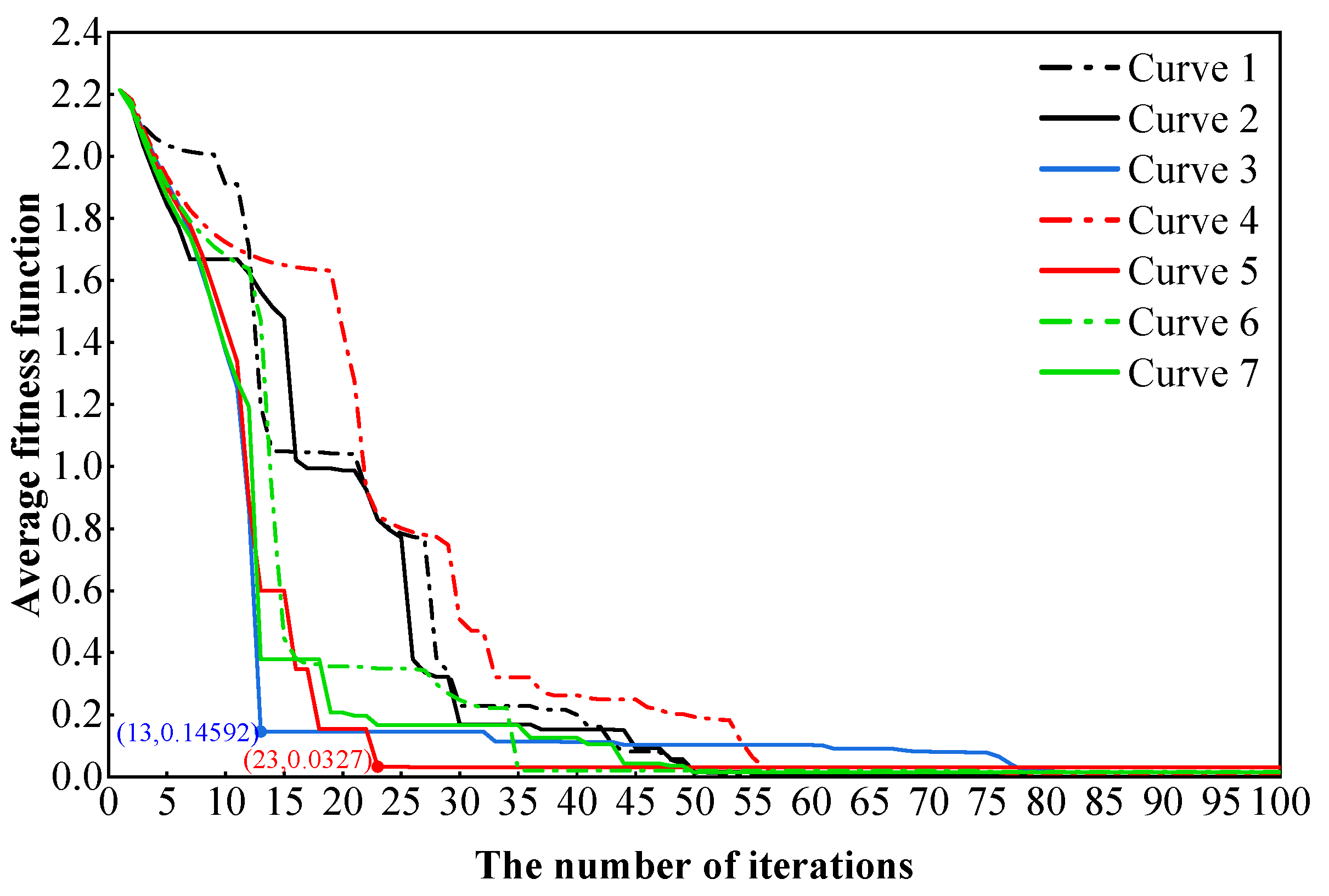
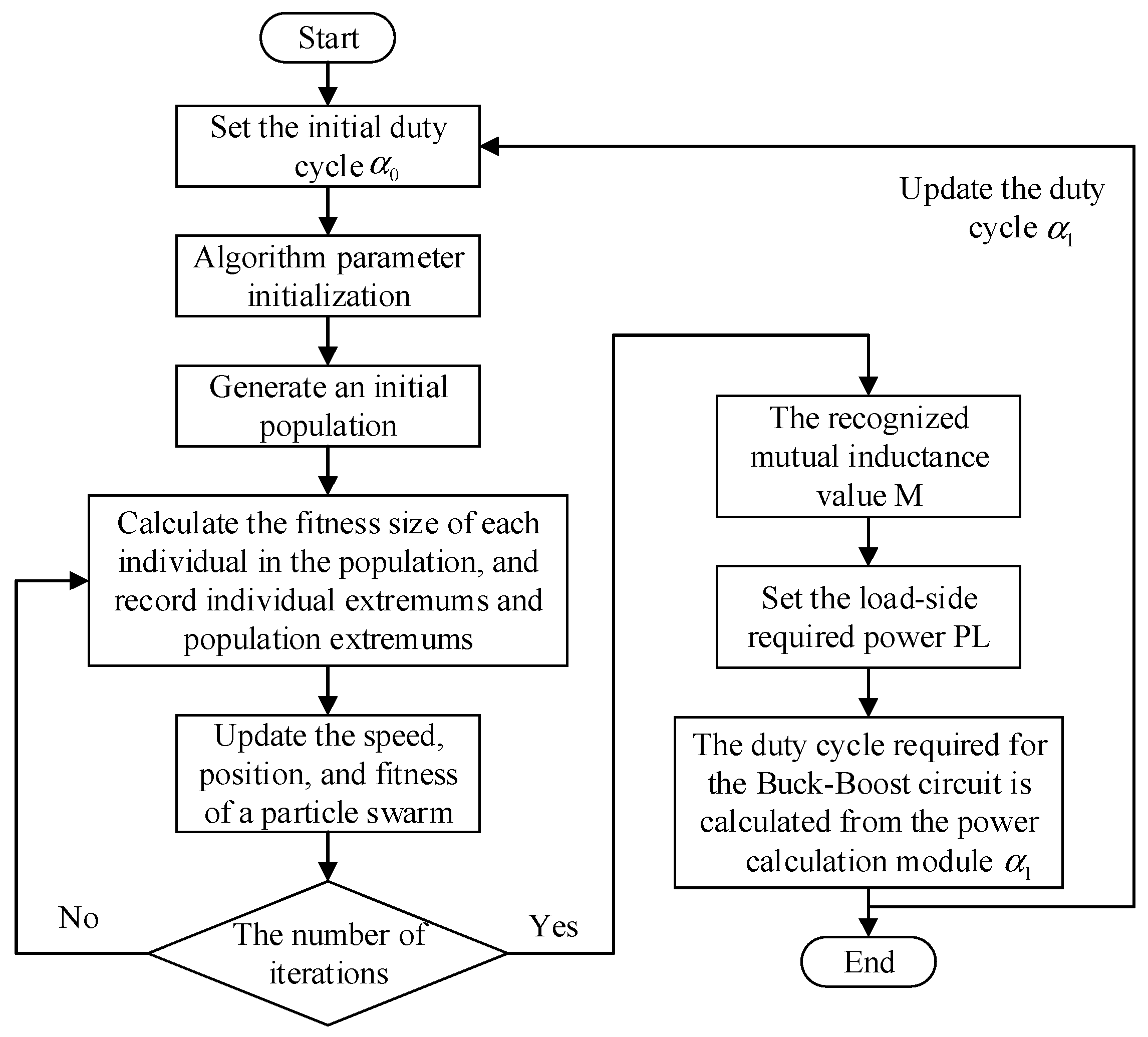
4.1. Improved Particle Swarm Algorithm

The PSO algorithm is an intelligent algorithm proposed by Kennedy and Eberhart in the USA in 1995 [27]. The algorithm is a global stochastic search algorithm. Through simulating the predatory behavior of a flock of birds, the search space for solving the problem is compared to the flight space of a bird. There is a group of n particles in an M-dimensional space, the current position of the particle can be recorded as x_i = (x_i1, x_i2, …, x_iM). Each particle searches independently for the optimal value in the search space, and the optimal value is recorded as the individual current optimal value P_gbest. Then, the individual optimal values are shared with the overall population, and the optimal adaptation value in the whole population is noted as the population’s current optimal value P_zbest. The population updates the speed and position of the particle swarm according to the found current optimal value P_gbest of the individual, the current optimal value P_zbest of the population, and the initial speed ${\nu }_{iM}^0$ for the next iteration. For each j-dimensional particle, the specific velocity and position are iterated as follows

$$\{\begin{array}{l}{\nu }_{ij}^{k+1}={\omega }_0{\nu }_{ij}^k+c_{1}rand(P_{gbest}-x_{ij})+c_{2}rand(P_{zbest}-x_{ij})\hfill \\ x_{ij}^{k+1}=x_{ij}^k+{\nu }_{ij}^{k+1}\hfill \end{array}$$

(21)

and

$${\omega }_0={\omega }_{\min }+({\omega }_{\max }-{\omega }_{\min })\frac{k}{k_{\max }},$$

(22)

where: k is the current iteration number, k_max is the maximum iteration number; ω₀ is the inertia weight, ω_min and ω_max are the inertia weight of the initial iteration and the inertia weight at the maximum iteration number k_max, usually ω_min and ω_max are 0.4 and 0.9 respectively [28]. i is the code name of a particle in the population. j is the dimension of the particle. ${\nu }_{ij}^{k+1}$ and $x_{ij}^{k+1}$ represent the k-th iteration, the velocity and position of the j-th dimension of particle i, respectively. c₁ and c₂ are the acceleration constants; rand is the random constant in [0,1].

According to Equation (21), it is possible to know that the algorithm’s initial inertia weight ω₀ should be large in order to quickly identify the ideal value range. The inertial weights ω₀ need to be small in the late stages of the algorithm, which makes it possible to determine the optimal value with a strong search power. Therefore, the inertia weight ω₀ should show a negative correlation with the number of iterations. The commonly used inertia weights ω₀ are linearly iterated according to Equation (22). Although the negative correlation is satisfied, the problems of slower search speed in the early stages, easier to fall into local optimum in the later stages and lower accuracy are more obvious. Therefore, the linearly decreasing function is modified to an exponential function in which the angle of inclination decreases with the number of iterations.

$${\omega }_0={\omega }_{\min }+({\omega }_{\max }-{\omega }_{\min })e^{-\frac{2k}{k_{\max }}}$$

(23)

Furthermore, in order to enhance the global search capability in the early stage and the local search accuracy in the later stage, the asymmetric synchronous learning factor is introduced with the original constant individual learning factor c₁ and social learning factor c₂. As the number of iterations of the algorithm increases, c₁ and c₂ change linearly.

$$\{\begin{array}{c}{c}_1=c_{10}-(c_{11}-c_{10})\frac{k}{k_{\max }}\\ c_2=c_{20}+(c_{21}-c_{20})\frac{k}{k_{\max }}\end{array}$$

(24)

In order to select a suitable initial value learning factor, multiple sets of simulation experiments are carried out, where the simulation fitness function is selected as the fitness function used in the recognition algorithm below. The simulation results are shown in Figure 10. Curve 1 and 2 are constant type learning factors, the difference is that Curve 1 uses Equation (22) to update the inertia weights, while Curve 2 uses an exponential function to update the inertia weights. Curve 3 is a symmetric linear learning factor c₁ = 2.5–0.5 and c₂ = 0.5–2.5, Curve 4 to 7 are asymmetric linear variations of c₁ = 2.5–0.5 and c₂ = 0.6–2.6, c₁ = 2.6–0.6 and c₂ = 0.5–2.5, c₁ = 2.5–0.5 and c₂ = 0.8–2.8, c₁ = 2.8–0.8 and c₂ = 0.5–2.5, respectively. From the simulation results, the introduction of exponential functions to update the inertia weights is beneficial in speeding up the PSO algorithm’s early search speed and later local search capability. PSO algorithms with linearly varying learning factors have higher overall search performance than constant PSO algorithms. Compared with the PSO algorithm with symmetrically varying learning factors, the PSO algorithm with asymmetrically varying learning factors is not only better in the first stage of the search but also has higher convergence accuracy in the later stage. In summary, the following recognition algorithm was selected for experiments with learning factors of c₁ = 2.6–0.6 and c₂ = 0.5–2.5.

4.2. Power Stabilization Control Strategy

On the basis of the improved PSO algorithm, this paper proposes a load power stabilization control strategy for LCC-S type MCR-WPT systems. The basic steps are shown in Figure 11.

Specific implementation steps.

Step 1: Set the initial duty cycle at α0.

Step 2: Parameter initialization. These include circuit para-meters: E_dc, r, L_f, C_f, C₁, C₂, R₁, R₂. L₁ and L₂ can be considered as fixed values from the above misalignment experiment. Algorithm parameters: Swarm size is 50, the maximum number of iterations are 100. On the basis of the misalignment simulation results in the Section 2, an appropriate margin is added as a constraint range for the mutual inductance identification algorithm: the mutual inductance range is from 25 µH to 50 µH and the load range is from 0 Ω to 12 Ω.

Step 3: Calculate the fitness function value of the first-generation individual. The fitness function e_j is chosen as the error between the calculated value of the inverter bridge output current I_{f_cal} and the true value I_{f_0}, I_{f_cal} where is obtained from the calculation of Equation (14). The fitness function e_j is

$$e_j=\left|I_{f\_cal}(M,R_L)-I_{f0}\right|$$

(25)

Step 4: Compare and record the current optimal value of the individual P_gbest and the current optimal value of the population P_zbest, and update the particle position and velocity according to Equations (21), (23) and (24) with boundary constraints.

Step 5: Determine whether the end condition is satisfied. If it is satisfied, output the mutual inductance identification result. Otherwise, continue to perform Step 3 to 4 until the end condition is satisfied.

Step 6: According to load side demand power P_L, calculate the duty cycle α1 required by the Buck-Boost circuit. The calculated value is given to the controller for control of the output power and the initial duty cycle value α0 is updated. When the system parameters change, repeat Step 1–6.

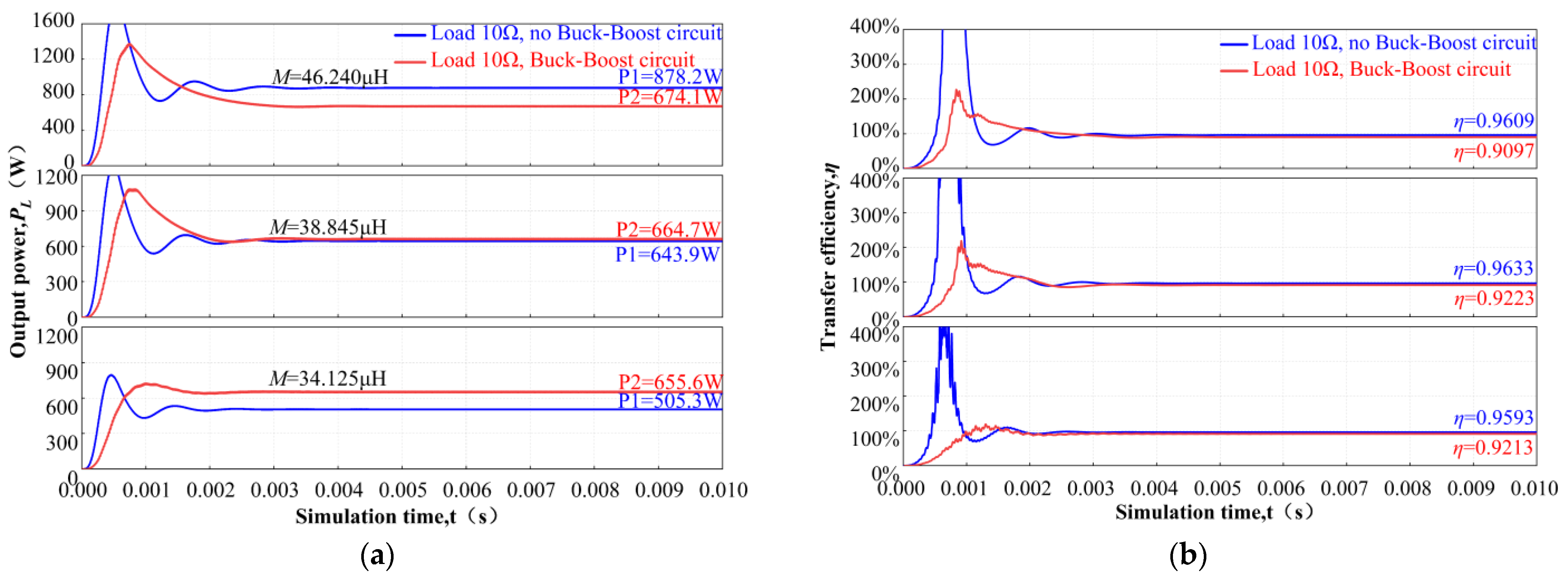
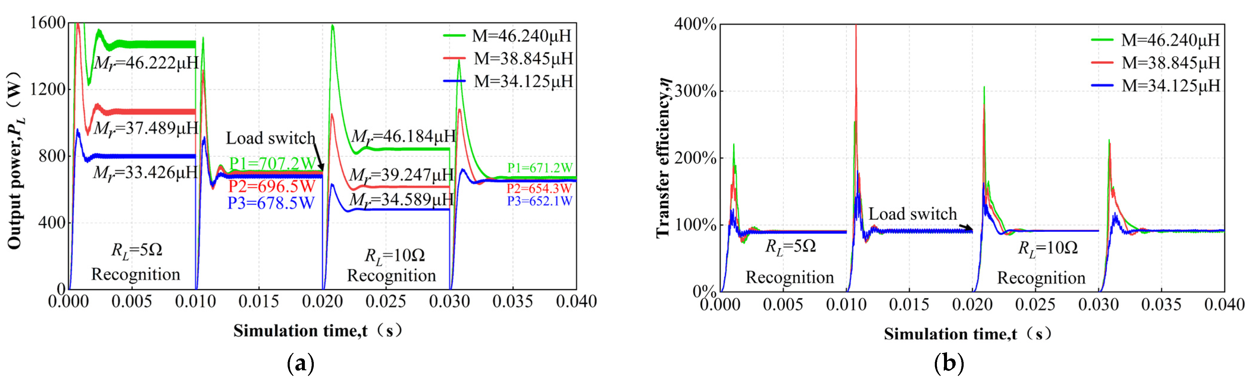
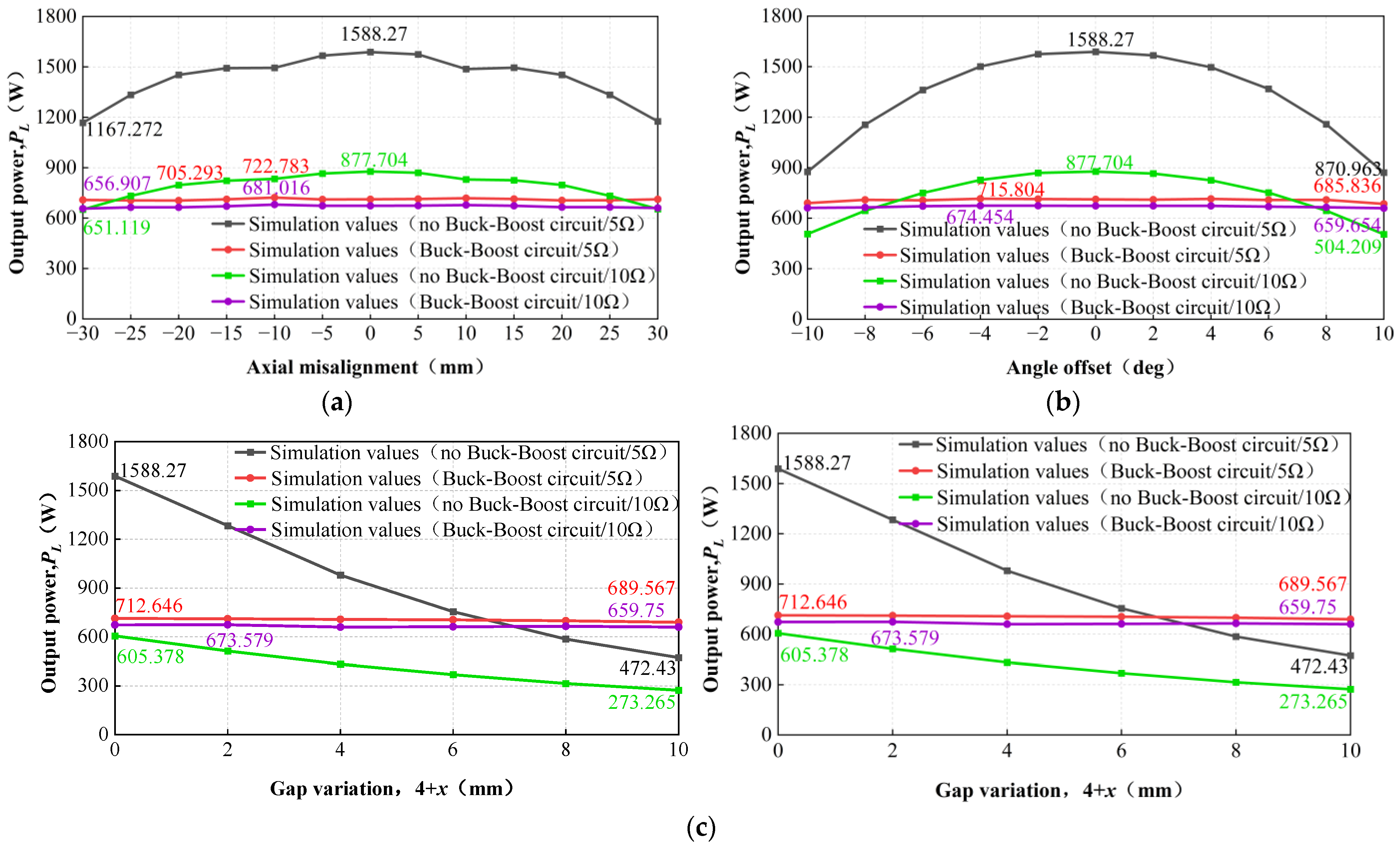
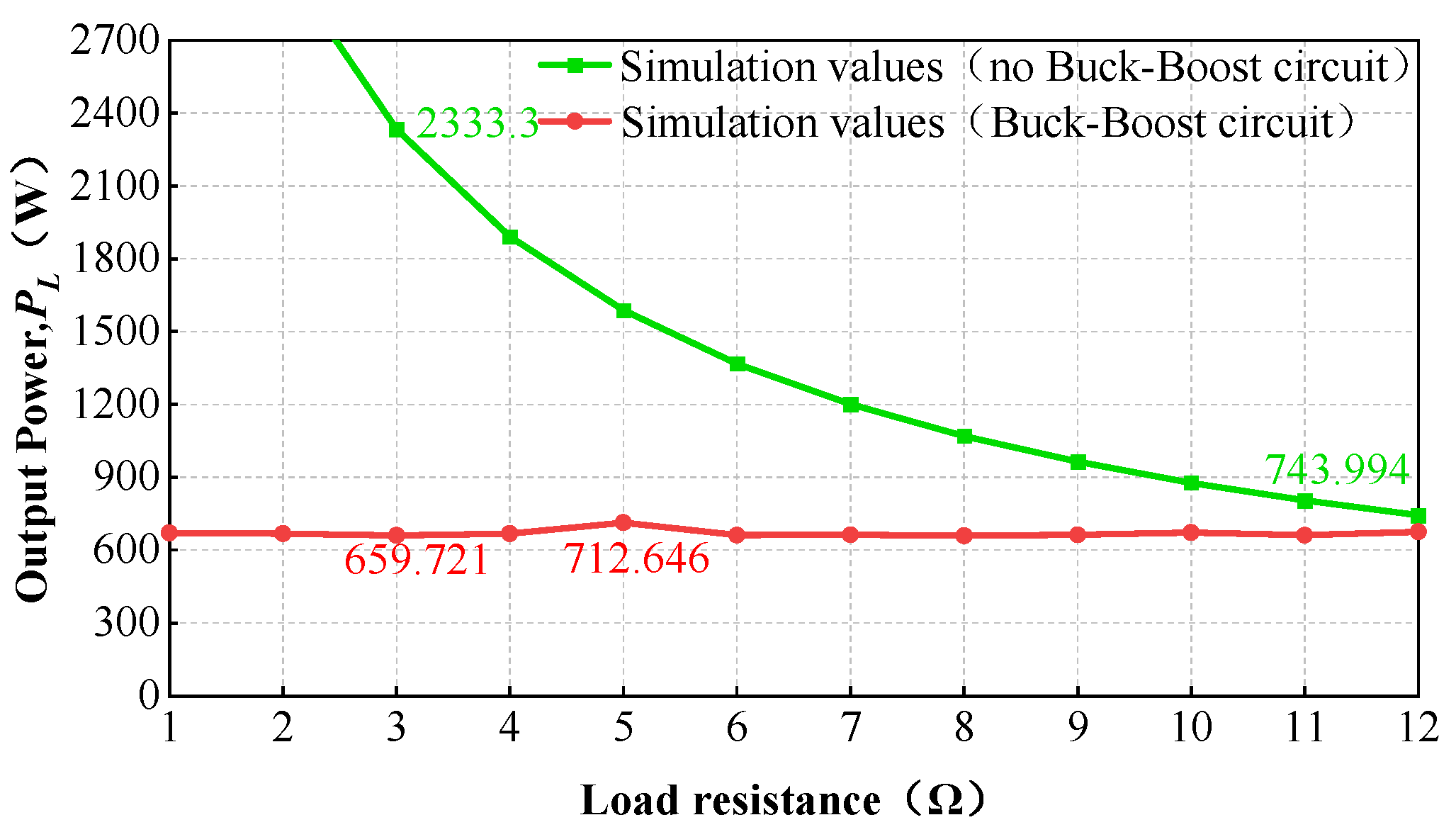
5. Simulation Analysis and Verification

To verify the effectiveness of the above mutual inductance identification algorithm and power stabilization strategy, a simulation model was built by Simulink. The basic parameters of the model, as shown in

Table 2. Parameters of the MC.

Symbol	Parameters	Value
Edc	DC Sources	80 V
r	DC source internal resistance	0.12 Ω
Lf	Primary series compensation inductance	37.5 μH
C1	Primary series compensation capacitor	167 nF
C2	Primary parallel compensation capacitor	270 nF
R1	Primary coil internal resistance	0.13 Ω
L1	Primary coil inductance	98.14 μH
L2	Secondary coil inductance	60.919 μH
R2	Secondary coil internal resistance	0.13 Ω
C2	Secondary series compensation capacitor	166 nF
f	system operating frequency	50 kHz

. The simulation time is set to 10 ms and the simulation step is set to 0.1 μs. The inverter current and voltage waveforms are shown in Figure 12.

Taking into account the requirements of the manufacturing process, magnetic coupling performance and adaptability to the underwater wireless charging environment, Mn-Zn ferrite was chosen as the magnetic core material. The coils were wound using a 450/750 V BVR flexible cable with 1.5 mm² insulation made of PVC, and the magnetic coupler was wound as shown in Figure 13. The magnetic coupler self-inductance, mutual inductance and resistance measurement tests were carried out using a Nikkei LCR measuring instrument IM3523, using both the paralleling and reversing methods (the average value was taken for multiple measurements) and the results are shown in

Table 3. Parameters of the new cores measured by the LCR measuring instrument.

Parameters	Expressions/Meanings	Values (Unit)
L1	Self-induction of the primary side	99.702 μH
L2	Self-induction of the secondary side	61.815 μH
L10	Self-induction by parallel method	246.620 μH
L20	Self-induction by reverse method	75.676 μH
M	$\left|(L_{10}-L_{20})/4\right|$	42.736 μH
k	$M/\sqrt{L_1{L}_2}$	0.544
R1	Equivalent resistance on the primary side	0.773 Ω
R2	Equivalent resistance on the secondary side	0.465 Ω

. As can be seen from the table, the wound physical cores are essentially the same as the parameters in Table 2, which verifies the coupling performance of the magnetic coupler.

To verify the effectiveness of the recognition algorithm, experiments were carried out by taking the average of multiple tests (10 times). The load resistance is 5 Ω and 10 Ω, record the mutual inductance identification values when the secondary and primary coils have axial, angle and gap misalignment respectively. The results are shown in Figure 13. As can be seen from Figure 14: the maximum and minimum relative errors for mutual sense identification are 2.35% and 0.1% respectively. When the load resistance is 5 Ω, the recognition accuracy of the three-dimensional misalignment is relatively high. When the load resistance is 10 Ω, the recognition accuracy is slightly lower, which is the main reason for the low control power when the load resistance is 10 Ω in the later section.

To verify the effectiveness of the power stabilization control strategy, it is necessary to compare the changes in output power P_L and efficiency η before and after the introduction of the control strategy. The experiments were carried out with the load of 10Ω and mutual inductances of 46.240 μH, 38.845 μH, and 34.124 μH respectively. The results are shown in Figure 15 (no Buck-Boost circuit in the figure means there is no power control strategy used, with Buck-Boost circuit means power control strategy is used). When the Buck-Boost circuit is not introduced, P_L changes by nearly 370 W, and η remains essentially at 96%. After the introduction of the power stabilization control strategy, P_L is maintained around 655 W to 674 W, the power change is only about 19 W and η is maintained at about 92%.

With different mutual inductance parameters and switching the load resistance from 5 Ω to 10 Ω, the variation of the system output power P_L and transmission efficiency η is shown in Figure 16. With a mutual inductance of 46.240 μH, 38.845 μH and 34.124 μH, the output power of the system can be maintained at around 680 W as the load resistance is switched. The maximum output power P_L reaches 707.2 W and the minimum is 652.1 W, with the relative error of 4.11% and 4.00%, and the efficiency η remains basically around 92.3%.

It is necessary to verify that the introduction of the control strategy has an effect on the stabilization of the system output power P_L, when axial, angle and gap misalignment occurs, and recording the variation of the output power under misalignment conditions. When the load resistance is 5 Ω and 10 Ω, the load side output power P_L is set to 680 W and the actual value of the system output power P_L when axial, angle and gap misalignment occurs is recorded. The results are shown in Figure 17. From the Figure 17, it is clear that when the primary and secondary coils are axially misaligned from −30 mm to 30 mm and when no control strategy is introduced, P_L fluctuates to 421 W and 226 W at the load 5 Ω and 10 Ω, with a relative fluctuation of 26.5%. After the introduction of the control strategy, P_L fluctuates between 705.2 W and 722.7 W, 656.9 W and 681.0 W at the load side, with a maximum relative fluctuation rate of 3.66%. When the primary and secondary coils are offset by −10° to 10° and the control strategy is not introduced, P_L fluctuations reach 718 W and 373 W at the load 5 Ω and 10 Ω, with a relative fluctuation rate of 45.2%. When the Buck-Boost power control circuit is introduced, P_L fluctuates between 685.8 W and 715.8 W, 659.6 W and 674.4 W at the load side, with the maximum relative fluctuation rate of 4.37%. As the gap between the primary and secondary coils changes from 0 mm to 10 mm and the control strategy is not introduced, P_L fluctuates between 1116 W and 332 W at the load 5 Ω and 10 Ω, with a relative fluctuation rate of 70.2%. Following the introduction of the Buck-Boost power control circuit, the output power fluctuates between 689.5 W and 712.6 W, 659.7 W and 673.5 W at the load side, with the maximum relative fluctuation rate of 3.35%. From the simulation results, it is evident that when no control strategy is used, P_L decreases rapidly as the degree of offset increases. The system’s output power P_L can be maintained around the set power after the introduction of the control strategy, which verifies the efficiency and accuracy of the control strategy.

In addition, during the AUV charging process, the load on the battery will change with factors such as environmental temperature. To simulate the effect of this process on system output performance, load variation experiments are required. While keeping the primary and secondary side without offset, load variations from 0 Ω to 12 Ω are tested and the change in system output power is recorded before and after the introduction of the power control strategy. The results are shown in Figure 18. Without the introduction of a control strategy, P_L fluctuates considerably. The lower the resistance of the load, the higher the output power. With the power control strategy, P_L fluctuates between 659.7 W and 712.6 W at the load side, and the maximum relative fluctuation rate is 4.90%. However, in the literature [29], using the power control strategy mentioned, the received power of the load fluctuates from a minimum value of 197.4 W to 210.3 W, with a stability rate of about 5%. Therefore, when the load resistance changes dynamically, the power control strategy proposed in this paper also has a strong and stable power output capability.

6. Conclusions

In this paper, an output power stabilization control strategy is proposed for an underwater wireless charging system. Firstly, a magnetic coupler with offset-resistant and highly fault-tolerant curved core structure is designed and analysed for misalignment and magnetic coupling capability by Maxwell software. Secondly, a parameter identification algorithm is proposed to identify the mutual inductance of the magnetic coupler in real time, by sampling the rms value of the inverter output current, the voltage and current towards the load sides to achieve parameter identification. Then, based on the parameter identification, real-time adjustment of the duty cycle of the rectifier-side Buck-boost circuit is used to control the output power. Finally, experiments are carried out to verify the correctness of the theoretical analysis. The results show that the designed curved core structure has excellent magnetic coupling capability in three-dimensional misalignment, and the mutual inductance identification algorithm can control the identification error within 2.5%, the control strategy power can be maintained at around 670 W, a maximum fluctuation rate is controlled within 4.9%. The designed magnetic coupler is highly attractive to precision devices such as unmanned aerial vehicles and AUVs that require miniaturisation on the receiving side, and the proposed control strategy based on the mutual sense identification algorithm has strong reference capability and significance for the stable transmission of wireless power.

References

1. Kadem, K.; Bensetti, M.; Bihan, Y.L. Optimal Coupler Topology for Dynamic Wireless Power Transfer for Electric Vehicle. Energies 2021, 14, 3983. [Google Scholar] [CrossRef]
2. Matsuda, T.; Maki, T.; Masuda, K. Resident autonomous underwater vehicle: Underwater system for prolonged and continuous monitoring based at a seafloor station. Robot. Auton. Syst. 2019, 120, 103231. [Google Scholar] [CrossRef]
3. Manikandan, J.; Akash, S.; Vishwanath, A.; Nandakumar, R.; Agrawal, V.K.; Manu, K. Design and development of contactless battery charger for underwater vehicles. Michael Faraday IET Int. Summit 2015, 2015, 362–367. [Google Scholar]
4. Zhou, J.; Li, D.J.; Chen, Y. Frequency selection of an inductive contactless power transmission system for ocean observing. Ocean. Eng. 2013, 60, 175–185. [Google Scholar] [CrossRef]
5. Lee, J.Y.; Han, B.M. A Bidirectional Wireless Power Transfer EV Charger Using Self-Resonant PWM. IEEE Trans. Power Electron. 2015, 30, 1784–1787. [Google Scholar] [CrossRef]
6. Wang, T.L.; Zhao, Q.C.; Yang, C.J. Visual navigation and docking for a planar type AUV docking and charging system. Ocean. Eng. 2021, 224, 108744. [Google Scholar] [CrossRef]
7. Sun, P.; Wu, X.S.; Cai, J.; Zhang, X.C.; Qiao, K.; Heng, S.H.M. Analysis of special technical problems of wireless charging at UUV docking stations and a new underwater electromagnetic coupler. Energy Rep. 2022, 8, 719–728. [Google Scholar] [CrossRef]
8. Cai, C.; Wu, S.; Zhang, Z.; Jiang, L.; Yang, S. Development of a Fit-to-Surface and Lightweight Magnetic Coupler for Autonomous Underwater Vehicle Wireless Charging Systems. IEEE Trans. Power Electron. 2021, 36, 9927–9940. [Google Scholar] [CrossRef]
9. Feezor, M.D.; Yates Sorrell, F.; Blankinship, P.R. An interface system for autonomous undersea vehicles. IEEE J. Ocean. Eng. 2001, 26, 522–525. [Google Scholar] [CrossRef]
10. Kojiya, T.; Sato, F.; Matsuki, H.; Sato, T. Automatic power supply system to underwater vehicles utilizing non-contacting technology. IEEE Techno-Ocean. 2004, 4, 2341–2345. [Google Scholar]
11. Zhang, Z.; Krein, P.T.; Ma, H.; Tang, Y.; Zhou, J.; Xu, D. An Inductive Power Transfer System Design with Large Misalignment Tolerance for EV Charging. In Proceedings of the 2018 IEEE 27th International Symposium on Industrial Electronics (ISIE), Cairns, Australia, 12–15 June 2018; pp. 1011–1016. [Google Scholar]
12. Kan, T.; Mai, R.; Mercier, P.P.; Mi, C.C. Design and Analysis of a Three-Phase Wireless Charging System for Lightweight Autonomous Underwater Vehicles. IEEE Trans. Power Electron. 2018, 33, 6622–6632. [Google Scholar] [CrossRef]
13. Lee, E.S.; Sohn, Y.H.; Choi, B.G.; Han, S.H.; Rim, C.T. A Modularized IPT With Magnetic Shielding for a Wide-Range Ubiquitous Wi-Power Zone. IEEE Trans. Power Electron. 2018, 33, 9669–9690. [Google Scholar] [CrossRef]
14. Mohamed, A.A.S.; Berzoy, A.; Mohammad, O. Magnetic design considerations of bidirectional inductive wireless power transfer system for EV applications. In Proceedings of the 2016 IEEE Conference on Electromagnetic Field Computation (CEFC), Miami, FL, USA, 13–16 November 2016; p. 1. [Google Scholar]
15. Mumtaz, F.; Yahaya, N.Z.; Meraj, S.T.; Singh, B.; Kannan, R.; Ibrahim, O. Review on non-isolated DC-DC converters and their control techniques for renewable energy applications. Ain Shams Eng. J. 2021, 12, 3747–3763. [Google Scholar] [CrossRef]
16. Le, K.; Hou, X.C.; Song, H. Mutual inductance estimation of multiple input wireless power transfer for charging stationary vehicles in parking spaces. AIP Adv. 2020, 10, 95–120. [Google Scholar]
17. Su, Y.G.; Chen, L.; Wu, X.Y.; Hu, A.P.; Tang, C.S.; Dai, X. Load and Mutual Inductance Identification from the Primary Side of Inductive Power Transfer System with Parallel-Tuned Secondary Power Pickup. IEEE Trans. Power Electron. 2018, 33, 9952–9962. [Google Scholar] [CrossRef]
18. Zheng, P.; Lei, W.; Liu, F.; Li, R.; Lv, C. Primary Control Strategy of Magnetic Resonant Wireless Power Transfer Based on Steady-State Load Identification Method. In Proceedings of the 2018 IEEE International Power Electronics and Application Conference and Exposition (PEAC), Shenzhen, China, 4–7 November 2018; pp. 1–5. [Google Scholar]
19. Sheng, X.; Shi, L. Mutual Inductance and Load Identification Method for Inductively Coupled Power Transfer System Based on Auxiliary Inverter. IEEE Trans. Veh. Technol. 2020, 69, 1533–1541. [Google Scholar] [CrossRef]
20. Gong, W.L.; Xiao, J.; Wu, X.R.; Chen, S.N.; Wu, N. Research on parameter identification and phase-shifted control of magnetically coupled wireless power transfer system based on Inductor–Capacitor–Capacitor compensation. Energy Rep. 2022, 8, 949–957. [Google Scholar] [CrossRef]
21. Chow, J.P.W.; Chung, H.H.; Cheng, C.S.; Wang, W. Use of Transmitter-Side Electrical Information to Estimate System Parameters of Wireless Inductive Links. IEEE Trans. Power Electron. 2017, 32, 7169–7186. [Google Scholar] [CrossRef]
22. Che, B. Omnidirectional wireless power transfer system supporting mobile devices. In Proceedings of the 2015 IEEE International Magnetics Conference (INTERMAG), Beijing, China, 11–15 May 2015; p. 1. [Google Scholar]
23. Cai, C.; Zhang, Y.; Wu, S.; Liu, J.; Zhang, Z.; Jiang, L. A Circumferential Coupled Dipole-Coil Magnetic Coupler for Autonomous Underwater Vehicles Wireless Charging Applications. IEEE Access 2020, 8, 65432–65442. [Google Scholar] [CrossRef]
24. Li, S.; Li, W.; Deng, J.; Nguyen, T.D.; Mi, C.C. A Double-Sided LCC Compensation Network and Its Tuning Method for Wireless Power Transfer. IEEE Trans. Veh. Technol. 2015, 64, 2261–2273. [Google Scholar] [CrossRef]
25. Li, Z.; Song, K.; Jiang, J.; Zhu, C. Constant Current Charging and Maximum Efficiency Tracking Control Scheme for Supercapacitor Wireless Charging. IEEE Trans. Power Electron. 2018, 33, 9088–9100. [Google Scholar] [CrossRef]
26. Zhang, M.; Tan, L.; Li, J.; Huang, X. The Charging Control and Efficiency Optimization Strategy for WPT System Based on Secondary Side Controllable Rectifier. IEEE Access 2020, 8, 127993–128004. [Google Scholar] [CrossRef]
27. Kennedy, J.; Eberhart, R. Particle swarm optimization. Int. Conf. Neural Netw. 1995, 4, 1942–1948. [Google Scholar]
28. Shi, Y.; Eberhart, R. A modified particle swarm optimizer. In Proceedings of the 1998 IEEE International Conference on Evolutionary Computation Proceedings, Anchorage, AK, USA, 4–9 May 1998; pp. 69–73. [Google Scholar]
29. Yang, X.; Wang, J.; Fei, Y.; Zhai, X.; Wang, C.; Zhang, M. Power stability control method of wireless power transfer system based on DC/DC circuit. Electr. Power Eng. Technol. 2019, 38, 173–178. [Google Scholar]
Figure 1. Planar single and bipolar emission magnetic field diagrams. (a) Unipolar magnetic field; (b) Bipolar magnetic field.
Jmse 11 00294 g001aJmse 11 00294 g001b
Figure 2. Overview of the cylindrical AUV and docking system.
Jmse 11 00294 g002
Figure 3. Schematic diagram of two structure sizes. (a) Arc-shaped core (Top view); (b) Double dipole core (Front view).
Jmse 11 00294 g003
Figure 4. Schematic diagram of misalignment.
Jmse 11 00294 g004
Figure 5. Static magnetic field clouds of two structures. (a) Arc-shaped core; (b) Double dipole core.
Jmse 11 00294 g005
Figure 6. Variation curves of mutual inductance M and coupling coefficient k with three-dimensional misalignment. (a) Axial misalignment; (b) Angle offset; (c) Gap variation.
Jmse 11 00294 g006
Figure 7. Diagram of the clamping device.
Jmse 11 00294 g007
Figure 8. The wireless power transfer system with LCC-S compensation.
Jmse 11 00294 g008
Figure 9. LCC-S type primary side equivalent circuit diagram.
Jmse 11 00294 g009
Figure 10. Diagram of average fitness values in Relation to initial values of learning factors c1 and c2.
Jmse 11 00294 g010
Figure 11. The flow chart of the power stabilization strategy based on the improved PSO mutual sense identification algorithm.
Jmse 11 00294 g011
Figure 12. Inverter output voltage and current simulation waveforms.
Jmse 11 00294 g012
Figure 13. Diagram of the magnetic coupling unit and the overall AUV system.
Jmse 11 00294 g013
Figure 14. Results of mutual inductance identification for different loads and three-dimensional misalignment. (a) Axial misalignment; (b) Angle offset; (c) Gap variation.
Jmse 11 00294 g014
Figure 15. Power and efficiency variation under different mutual inductance for a load of 10 Ω. (a) Output power; (b) Efficiency.
Jmse 11 00294 g015
Figure 16. Variation in output power and efficiency when switching loads with different mutual inductance. (a) Output power; (b) Efficiency.
Jmse 11 00294 g016
Figure 17. Power control curve for axial, angle, and gap offset. (a) Axial misalignment; (b) Angle offset; (c) Gap variation.
Jmse 11 00294 g017
Figure 18. Output power curve under different resistance loads.
Jmse 11 00294 g018