Abstract
This study presents morphological data and estimates of the settling velocity and drag coefficient of sea stars (Asterias rubens) caught in the Limfjord, Denmark. A geometric model describing the sea star is presented and the thickness and arm width are determined as linear functions of arm length. The volume and mass of the sea stars is well predicted by the geometric model and is in agreement with the experimental measurements. The mean sea star density is determined to be 1095 kg/m3, the mean drag coefficient is estimated to be 2.3 and the settling velocity is shown to vary with the square root of the its size.
1. Introduction
Globally, sea stars are major predators of molluscs and other benthic invertebrates and can have considerable impact on cultivated beds and natural populations of shellfish species, such as mussels, oysters, scallops and clams. Consequently, several methods have been developed to protect shellfish beds from sea stars, including mopping, dredging, trapping, fencing and hand-picking [1].
The most common sea star in the northeastern Atlantic Ocean is the common sea star (Asterias rubens), whose range extends from Norway to Senegal [2]. It can occur in very large numbers and can pose a particular threat to blue mussel (Mytilus edulis) and scallop (Pecten maximus) fisheries [3,4,5]. Trawling is one of the methods used by fishers in northwestern Europe to catch the common sea star. While the original intention of trawling for sea stars was to remove them from shellfish beds, in recent years a sea star fishery has developed in its own right. They are high in protein, and can be exploited as a marine-based protein supplement for animal feed.
When trawl gears are used on top of bottom culture beds, large amounts of mussels can be fished as a bycatch. Hence, efforts have been made to develop trawl fishing gear which minimize these impacts. One such method is to use the hydrodynamics around the gear components that are towed close to the seabed to lift sea stars into the water column rather than lifting them mechanically with seabed-contacting gear components. Computational fluid dynamics (CFD) can predict how the trawling hydrodynamics affects sea stars, provided there is knowledge about their morphological dimensions (e.g., their projected surface area, volume and density) and settling velocity. This allows us to model the trajectory of the sea stars. The biology and ecology of Asterias rubens has been investigated by [6,7], and much is known about their sexual maturity, spawning and growth rate [8,9,10]. Detailed studies to describe their response to gravity [11], water current [12] and extracts of Mytilus edulis [13] have also been conducted, but little is known specifically about the density and settling velocity of the common sea star. Ref. [14] used a CFD model to investigate how sea stars, with an idealized shape, generate a downward force to keep them attached to surfaces. They likewise estimated their drag coefficient when aligned with the flow in a study on the kinematics of sea star locomotion. Ref. [15] additionally measured the density of Asterias forbesi, a less common sea star in the northeastern Atlantic.
The present study measures the morphology, volume and mass of Asterias rubens and estimates its density. We also carry out experiments to measure its settling velocity and to determine its drag coefficient while falling through the water column, prerequisites for detailed hydrodynamic modeling of sea stars.
2. Material and Methods
2.1. Specimen Collection
Sea stars were collected from the Limfjord, Denmark on 10 and 30 March 2022. The specimens were randomly sampled from the catches of a commercial boat while trawling for sea stars. The hauls on March 10 were performed on both cockle (Cerastoderma edule) and blue mussel (Mytilus edulis) beds. A total of 1486 sea stars were collected (group 1) and their length measured. A further 125 sea stars were collected from the last haul (group 2) and brought back ashore for the settling velocity experiments. Ashore, these sea stars were kept in a laboratory tank to keep them alive and in similar conditions as in the fjord. The sea stars were left overnight in the laboratory tank to reduce their stress after being trawled, and measurements were performed the day after collection. More specimens were collected on 30 March 2022 consisting of 136 sea stars (group 3) on which biometric measurements were conducted. This group was also left overnight in the laboratory tank before the measurements were performed.
2.2. Biometric Measurements
The length of the sea stars (L) was measured from the middle of the central disc to the tip of an arm to the nearest half centimeter, see Figure 1. The measured size of the central disc () is characterized by the distance from one armpit to an armpit two arms away while the thickness (T) was measured at the central disc. The central disc and the thickness were measured with a caliper to the nearest millimeter. The arm width (), defined as the widest place on the arm (see Figure 1), was also measured, for a subgroup of 117 sea stars from group 3.
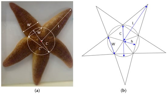
Figure 1.
Common sea star (Asterias rubens) picture and geometric model. (a) Sea star with definition of the measured arm width , size of central disc and length L. (b) The geometric sea star model with definition of arm width W, diameter of central disc C and length L. The apothem of the pentagon inscribed by the central disc h is used in (2.3) to derive an expression for the area of the geometric model.
Sea stars move using a hydraulic system, which drains if they are taken out of the water. Hence, to find the mass of sea stars in their natural habitat, it is important to ensure that the drained water is included in the measurement. This was accomplished by placing a container underneath the sea stars immediately after they were taken out of the water, which were then weighed, using an electronic balance to the nearest gram. The volume of the sea stars was measured using a container with an overflow. Water was filled up to the overflow, after which the sea stars were lowered into the container. Water corresponding to the volume of the sea star then ran into another container through the overflow tube. The mass of the excess water was measured, and the volume was determined by , where the seawater density is kg/m3.
2.3. Geometric Sea Star Model
In this study the sea stars are modeled as a regular pentagon and five isosceles triangles as sketched in Figure 1b. The diameter of the central disc C, the arm width W and arm length L are indicated on the figure, as well as the apothem of the pentagon h. Due to practical reasons, the size of the central disc is measured instead of the diameter of the disc C. The relation between the measured size of the central disc and the diameter of the central disc C is given by the geometry of the modeled sea star as
Similarly, the relationship between the width of the isosceles triangles W and the diameter of the central disc is given as
The area of the modeled sea star is given by
which is also an estimate of the largest projected area (the frontal projection) of the common sea star. Provided the average thickness (from center to the tip of the arms) is proportional to the measured thickness, then it follows that the volume of the common sea star can be estimated by
Here the proportionality factor is presently unknown but will be determined in Section 3.
2.4. Settling Velocity Experiment
The settling velocity experiment was conducted using the group 2 sea stars. Figure 2 shows a sketch and a snapshot from the settling velocity experiment. A tank, with a diameter of 56 cm at the window section, a height of 96 cm and a 25 × 50 cm acrylic window, was filled with filtered (60 μm) seawater from the Limfjord. The water level in the tank was at least 20 cm above the window. A video camera was placed approximately 1 m from the tank and in front of the window. Two rulers were inserted in the centerline of the tank approximately 15 cm apart. They were positioned such that the numbers could be read in the video and used for calibrating position. The camera had a frame rate of 30 frames per second. The sea stars were dropped in a horizontal position just underneath the water surface. After the sea stars were released, they would accelerate before obtaining a constant (terminal) velocity, the settling velocity. The sea stars were filmed while falling through the water column with a video camera. Their motion was tracked using a post-processing tool, where the position of the sea star was determined at every fifth frame. A point in one of the armpits was chosen for each sea star to represent its position, and the corresponding horizontal and vertical coordinates () were determined as functions of time by translating pixels to position using the rulers. The settling velocity of each specimen was determined as the rate of change in position after reaching terminal velocity.
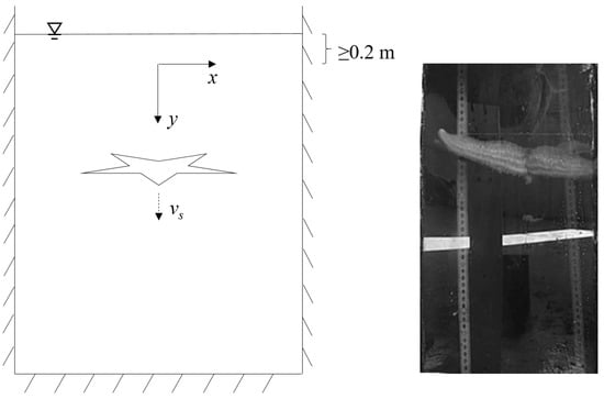
Figure 2.
Sketch and snapshot of the settling velocity experiment.
2.5. Drag Coefficient
The drag coefficient quantifies the resistance of an object in a flowing fluid environment. It is a dimensionless quantity and it is related to the drag force by
following Equation (2.8) in [16]. The drag force is equal to the combined action of gravity and buoyancy, i.e., the submerged weight of the body when the sea star has reached terminal velocity. Equating these and rearranging, the drag coefficient can be expressed as
where m/s2 is the gravitational acceleration and the largest frontal projection A is taken as (3).
Formally, the drag coefficient should be a function of the shape of the body and the flow regime defined by the Reynolds number
where m2/s is the kinematic viscosity of the seawater.
3. Results
3.1. Distribution of Lengths
The lengths of 1486 sea stars (group 1) were measured, of which 609 were sampled from cockle beds and 877 from blue mussel beds. They ranged in length from 2.5 to 15 cm. Their length probability density functions are similar with mean values of 10.3 and 9.7 cm for cockle and mussel bed, respectively, see Figure 3. Both distributions have a small group of individuals with lengths around 2.5–6 cm and a larger group from 6–16 cm. The life span of Asterias rubens is 7–8 years (Schäfer 1972), where the growth rate is most rapid in the first couple of years [10]. The growth rate of Asterias rubens is highly dependent on food supply, and starvation can even cause shrinkage [9]. The plasticity of the growth rate causes difficulties in age determination, which cannot be inspected by growth rings [17]. However, the small local peak for smaller L suggests a year class with a length of about cm, while the global peak has a length of about cm.
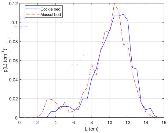
Figure 3.
Probability density functions based on 609 individuals sampled on cockle beds and 877 on mussel beds (group 1).
3.2. Width and Thickness
The arm width of the sea star W was not directly measured. However, it can be estimated from the measured and as follows. First, the relation between the measured arm width and , where C is defined by (1), is established. Figure 4 shows this ratio (i.e., the relationship between and ) as a function of length. It suggests that there is a fixed ratio between the thickest point on the arm and . The relation based on the mean value can be established as
It should be emphasized that the ratio is based on the measurements of the central disc and the arm thickness at the thickest point. By knowing this ratio, the arm width in the model W can be determined only from the measured arm width as
given the relation between C and W in (2).
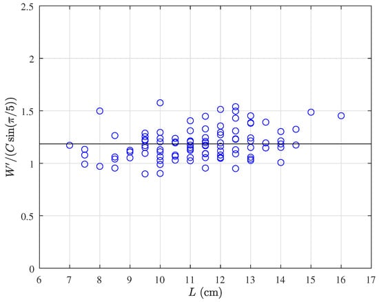
Figure 4.
Ratio of measured arm width of Asterias rubens and the size of the central disc scaled with . The solid line corresponds to (8).
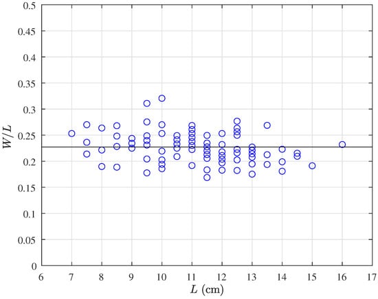
Figure 5 shows the non-dimensionalized arm width as a function of length, where the data points are calculated using (9) from . The data support that is approximately constant, with the mean being
which is depicted as the solid line.
The measured dimensionless thickness of the sea stars is shown in Figure 6 as a function of the length L. To a first approximation, a dimensionally consistent relation between the thickness and length can again be found from the mean value
The relation is represented in the figure as a solid line. Note that a linear relation is chosen for the thickness as a function of length to maintain dimensional consistency, which is needed for the forthcoming determination of volume and density.
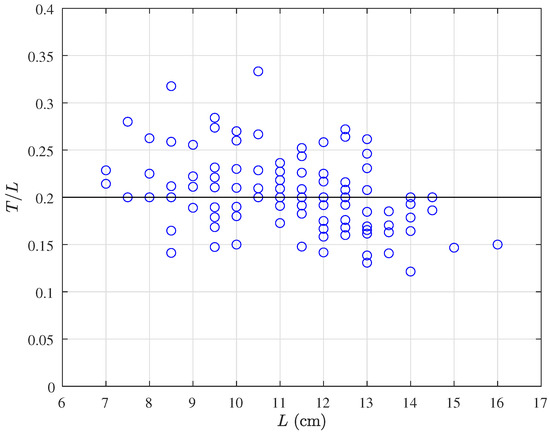
Figure 6.
Measured thickness of Asterias rubens as a function of length. The solid line corresponds to (11).
3.3. Volume and Density of Sea Stars
Using the proposed geometric sea star model, the volume should be proportional to the product of the area and thickness as expressed in (4). Figure 7 shows the ratio of the measured volume of the sea stars to , as defined in (4), and the measured thickness as a function of length. The proportionality factor is, from this, determined as
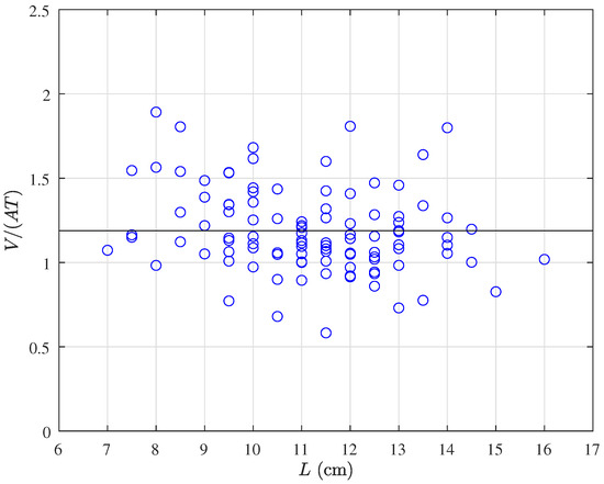
The thickness of the sea star was measured at the central disc, however, the thickness changes along the length of the arm. The proportionality factor in excess of unity accounts for geometric aspects such as this, and the fact that the area A is only an estimate.
Invoking (3), (10) and (11) into (12) now yields the following dimensionally consistent expression for the sea star volume
Figure 8 checks the validity of (13) by plotting the measured volume of the sea stars as function as length. Equation (13) is depicted as the solid line and confirms good agreement between the geometric model and the measurements.
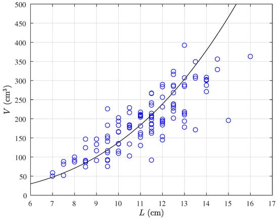
Figure 8.
Measured volume of Asterias rubens as a function of length. The solid line corresponds to (13).
The uncertainty of the volume measurement is estimated to be ±5 cm3 due to surface tension at the overflow and drops on the container used for the overflow water. The volume measurements were performed on group 3, and sea stars having a length smaller than 7 cm were removed to ensure an accuracy of at least 10%.
The mass and volume measurements were performed on the same group of sea stars and can be combined to determine the density of the sea stars. Figure 9 shows the density of the sea stars as a function of length. To a first approximation, the density of the common sea stars (once outliers of more than two standard deviations have been removed) is determined to be
which, as expected, is larger than the water density in the experimental conditions, namely 1022 kg/m3. The density of the common sea star is less than that obtained by [15] for Asterias forbesi, which they estimated to be in the range 1110–1154 kg/m3. This difference, however, is not surprising, given that it is for a different species, in a different location, and potentially at a different time of year.
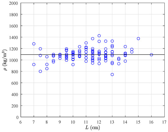
Figure 9.
Density of Asterias rubens calculated for each individual. The solid line corresponds to the mean density.
It should be noted that these experiments were conducted in March, when the common sea stars are pre-spawning and contain significant amounts of eggs and sperm. Hence, there may be a seasonal variation in density, which is not accounted for in the present study.
3.4. Mass–Length Relationship
The mass can be determined from the volume and density as
The volume and density of the sea stars have been determined in (13) and (14), respectively, hence the mass can be modeled as
The measured mass M of the sea stars is shown in Figure 10 as a function of length L together with the modeled mass (16) shown as the solid line. As with the volume, the measured mass is well-predicted by the model. The mass of Asterias rubens was likewise investigated by [6]. In their study, the sea stars were caught in two different ways: by divers and trawl. Both of their data sets are also shown in Figure 10 (green squares and red diamonds). A reanalysis of the data from [6] has been conducted to obtain dimensionally correct predictive models for their two data sets with the same accuracy as in the present study. These two predictive models are shown as dashed and dotted lines in the figure with expressions given in the legend. The present data set lies between those used in [6]. Here we point out that the large sea stars are closer to the trawl-caught data, whereas the small sea stars are closer to the dive-caught data. This is discussed further in Section 4.
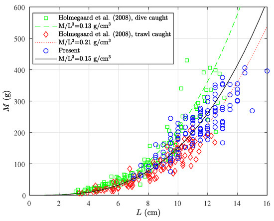
Figure 10.
Measured mass of Asterias rubens. The solid black line corresponds to (16). Other data are from [6].
3.5. Drag Coefficient and Settling Velocity
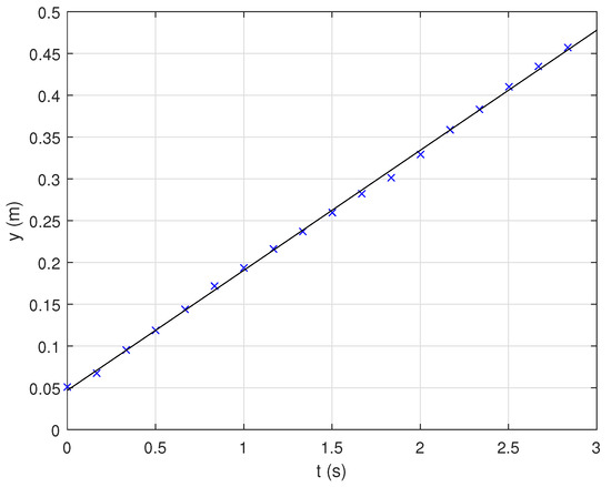
Figure 11 shows a sample recording from the measurements of a sea star falling through the water column at several time steps. The sea stars were released close to this preferential settling orientation. After being let go, the sea star tilted slightly from the horizontal position and slid to one side while moving downwards. The tilt of the sea star decreased until it returned to a horizontal position and a maximal displacement in the x-direction is obtained. Hereafter, the sea star tilts in the opposite direction and the sliding in the x-direction starts to reverse, eventually reaching another maximum displacement in the x-direction, at which point the process repeats. This zig-zag path through the water column is like that of a leaf or a card falling through air [18,19]. There is also rotation around the y-axis, however, the main motion is in the y-direction, which is the only one needed to obtain the settling velocity, . The y-position of the sea star, shown in Figure 11, is given as function of time t in Figure 12. The settling velocity is determined as the slope of the linear fit to the measurement points.
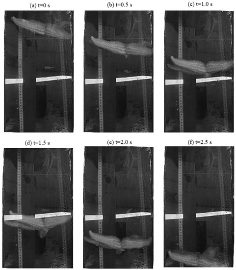
Figure 11.
Snapshots of a sea star falling through water column in the settling velocity experiment.
The drag coefficient is determined from (6), where the modeled area, density, volume and measured settling velocity are used. Figure 13 shows the drag coefficient as a function of the Reynolds number. The density and volume were only given to a first approximation, which means that the drag coefficient, within reason, can only be estimated as a constant, such that
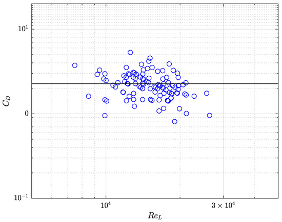
Figure 13.
Drag coefficient as a function of Reynolds number for Asterias rubens. The solid line corresponds to (17).
Isolating for the settling velocity in (6) gives the following model
where V is given by (4), A is given by (3) and is given by (17), i.e., it predicts a settling velocity that varies with the square root of the thickness. The thickness is shown to be proportional to the length L in (11), hence the settling velocity varies with the square root of L. Figure 14 shows that there is good correspondence between the measured settling velocities and the predictions of (18).
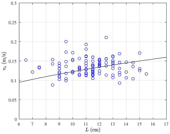
Figure 14.
Measured settling velocity of Asterias rubens as a function of length. The solid line corresponds to (18).
4. Discussion
The geometric sea star model proposed in the present study is simple yet elegant. While it assumes that arm width and thickness are linearly related to length, the resulting models of mass and volume fit the experimental data well, while maintaining dimensional homogeneity. However, it should be noted, that the area given by the model is slightly less than for a real sea star since the arms are modeled as isosceles triangles being thickest where they are attached to the pentagon. For the real sea star, the arm was seen to be wider further from the central disc. This leads to an underestimation of the area and hence an overestimation of the drag coefficient. The settling velocity of sea stars will, however, be unaffected.
It should be noted, that mass was seen to be dependent on the catchment method, where sea stars caught by divers are less stressed and closer to in-situ conditions. This is apparent from Figure 10, where the measurements in the present study are seen to be in-between the measurements performed by [6]. The sea stars caught by divers will have experienced minimal stress, while the trawl-caught sea stars would have experienced a lot of stress. This is seen by a reduction of mass for the trawl-caught sea stars. In the present study the sea stars were caught by trawl but had time to recover from the stress in the laboratory and re-hydrate before the measurements were performed. This may explain why the present data set lies between those of [6]. The data points for the large sea stars are closer to the trawl-caught data, whereas the small sea stars are closer to the dive-caught data. This suggest that the large sea stars do not recover as well as the small sea stars. The predictive model, presented in the present study, applies to the study by [6] once the effect of the catchment method is accounted for. From the reanalysis of the two data sets in [6], the expected mass range was 0.13 g/cm3 ≲ ≲ 0.21 g/cm3. While (15) is dimensionally homogeneous, this is not. The unknown density in [6] does not allow their result to be presented in a dimensionally homogeneous fashion. However, the presumption is that the common sea star loses mass due to fluid being drained when stressed (e.g., when caught using trawls). If the fluid drained is sea water (or has a density close to sea water), then this would suggest that the density of the sea star changes with the change in mass. With this assumption, it is possible to estimate the change in density from the present data set. This approach suggests that the density of in-situ sea stars (dive-caught) may be as small as 1073 kg/m3, while the density of sea stars caught with a trawl may be as high as 1107 kg/m3. The density is a parameter that affects the settling velocity, as indicated by (17), hence changes in the density of the sea star will impact the settling velocity. However, this is inherently handled by the predictive model as formulated in the present study.
The mass–length relationship of 1773 fish species in [20] was found to be proportional to . The coefficient was found to be in the range and the coefficient for the sea star (Pentaceraster regulus) in [21] was found to be . The original fit in [6] suggests = 2.7. In the present study, the precision in the morphology measurements and the requirement for a homogeneous model do not allow more than a linear relation between the arm width–length or thickness–length ratios, hence the volume and mass must be proportional to . An added bonus of volume and mass being proportional to is that it yields a dimensionally homogeneous model.
The tank used for the settling velocity experiment had a diameter of 56 cm, giving a cross-sectional area of 0.246 cm2 while the largest investigated specimen had a cross-sectional area of 0.0188 cm2. The blockage ratio, i.e. the ratio between the area of the sea star and the tank, is 7.6%. From [22], a blockage ratio less than 6% will have a negligible effect on the drag coefficient, while a high blockage can create considerable distortion of the flow with complex effects. The blockage in the experiment is only slightly higher than the estimated 6%, and only for the largest sea stars, and hence is assumed to have an insignificant effect.
Modeling how sea stars are affected by hydrodynamics requires a priori knowledge of their morphology, density and settling velocity (or drag coefficient). The present model, Figure 1b and Equations (10)–(12), (15), (17) and (18), provide this information. Using the hydrodynamics of towed near-bed gear components to lift sea stars from the seabed requires that the induced lift force is large enough to overcome the submerged weight and the suction from the tube feet of the sea stars. This can be analyzed with a CFD model given the present morphology and settling velocity model. Once sea stars are suspended in the water column, their trajectory is directly affected by the hydrodynamics behind the fishing gear, and the lateral motion and settlement of the sea stars can be predicted by combining a CFD model with the present morphology model. Knowing the most likely path the sea stars will follow allows fishing gear to be configured to increase the efficiency and potentially reduce bycatch, such as shellsfish. Ref. [23] Siemann et al. (2021) used such an approach to help design a scallop dredge that caught fewer flounder. Ref. [24] measured the settling velocity of a number of sea shells and found values in the range 0.16–0.22 m/s. Combining this type of information with the results of the present study, gear could be designed that both optimizes the catch of more slowly falling sea stars and avoids retention of faster falling shells.
5. Conclusions
The morphology and settling velocity of the common sea star has been measured experimentally. The size distribution of Asterias rubens was determined for samples from mussel and cockle beds, based on 609 and 877 sea stars, respectively. The mean values of the distributions for the cockle and muscle bed were 10.3 cm and 9.7 cm, respectively, and the modes of the distributions for arm length were around 11 cm. The arm width and thickness of the sea stars were determined as a function of length and a geometric model describing the sea star as a regular pentagon with 5 isosceles triangles was created. The volume and mass of the sea stars is well predicted by the geometric model, and the mean density of the sea stars was determined to be kg/m3. Furthermore, the drag coefficient was found to be = 2.3 and it was used to convincingly predict the settling velocity of the common sea star. The settling velocity is shown to vary with the square root of the length of the sea star.
Author Contributions
Data curation, K.B.B.; Formal analysis, K.B.B., S.C., D.R.F. and F.G.O.; Funding acquisition, S.C., D.R.F., C.S. and F.G.O.; Methodology, K.B.B., S.C., D.R.F., C.S. and F.G.O.; Project administration, F.G.O.; Supervision, S.C., D.R.F., C.S. and F.G.O.; Writing—original draft, K.B.B.; Writing—review & editing, K.B.B., S.C., D.R.F., C.S. and F.G.O. All authors have read and agreed to the published version of the manuscript.
Funding
The research leading to these results has received funding from the European Fisheries Fund and is part of the project “Using hydrodynamics to develop more selective fishing gears” (HydroSel), Grant number 33113-I-19-130, and the project “Kulturbanker—udvikling af nye skånsomme metoder i muslingefiskeriet” (KulturMus) funded by GUDP, Grant 34009-19-1528.
Institutional Review Board Statement
During the handling of experimental animals, care was taken to prevent unnecessary suffering. Sea stars are invertebrate and are not included in the definition of animals under Directive 2010/63/EU of the European Parliament and the Council on the protection of animals used for scientific purposes.
Informed Consent Statement
Not applicable.
Data Availability Statement
The data presented in this study can be found at doi:10.11583/ DTU.20160488.
Acknowledgments
We are grateful to Peter Skou Dalsgaard for his assistance in collecting the specimens and the Danish Shellfish Center for lending us the required equipment. We are also thankful to Kasper Meyer for his help sampling and his valuable comments and suggestions.
Conflicts of Interest
The authors declare no conflict of interest.
References
- Barkhouse, C.; Niles, M.; Davidson, L.A. A literature review of sea star control methods for bottom and off bottom shellfish cultures. Can. Ind. Rep. Fish. Aquat. Sci. 2007, 279, 1–44. [Google Scholar]
- Budd, G.C. Asterias rubens Common Starfish. 2022. Available online: https://www.marlin.ac.uk/species/detail/1194 (accessed on 18 June 2022).
- Calderwood, J.; O’Connor, N.E.; Roberts, D. Efficiency of starfish mopping in reducing predation on cultivated benthic mussels (Mytilus edulis Linnaeus). Aquaculture 2015, 452, 88–96. [Google Scholar]
- Magneson, T.; Redmond, K.J. Potential predation rates by the sea stars Asterias rubens and Marthasterias glacialis, on juvenile scallops, Pecten maximus, ready for sea ranching. Aquac. Int. 2012, 20, 189–199. [Google Scholar]
- Dare, P.J. Notes on the swarming behaviour and population density of Asterias rubens L. (Echinodermata: Asteroidea) feeding on the mussel, Mytilus edulis L. J. Cons. Cons. Perm. Int. Pour L’Explor. Mer. 1982, 40, 112–118. [Google Scholar] [CrossRef]
- Holtegaard, L.E.; Gramkow, M.; Petersen, J.; Dolmer, P. Biofouling og Skadevoldere: Søstjerner; Technical Report; Dansk Skaldyrscenter: Nykøbing Mors, Denmark, 2008. [Google Scholar]
- Sloan, N.A. Aspects of the feeding biology of Asteroids. Oceanogr. Mar. Biol. Annu. Rev. 1980, 18, 57–124. [Google Scholar]
- Orton, J.H.; Fraser, J.H. Rate of growth of the common starfish, Asterias rubens. Nature 1930, 126, 567. [Google Scholar] [CrossRef]
- Vevers, H.G. The Biology of Asterias Rubens L.: Growth And Reproduction. J. Mar. Biol. Assoc. UK 1949, 28, 165–187. [Google Scholar] [CrossRef]
- Nichols, D.; Barker, M. Growth of juvenile Asterias rubens L. (Echindermata: Asterioidea) on an intertidal reef in southwestern Britain. J. Exp. Mar. Biol. Ecol. 1984, 78, 157–165. [Google Scholar] [CrossRef]
- Castilla, J.C. Responses of Asterias rubens to gravity. Behaviour 1975, 72, 84–94. [Google Scholar] [CrossRef]
- Castilla, J.C.; Crisp, D.J. Responses of Asterias rubens to water currents and their modification by certain environmental factors. Neth. J. Sea Res. 1973, 7, 171–190. [Google Scholar] [CrossRef]
- Castilla, J.C.; Crisp, D.J. Responses of Asterias rubens to olfactory stimuli. J. Mar. Biol. Assoc. UK 1970, 50, 829–847. [Google Scholar] [CrossRef]
- Hermes, M.; Luhar, M. Sea stars generate downforce to stay attached to surfaces. Sci. Rep. 2021, 11, 4513. [Google Scholar] [CrossRef]
- Ellers, O.; Khoriaty, M.; Johnson, A.S. Kinematics of sea star legged locomotion. J. Exp. Biol. 2021, 224, jeb242813. [Google Scholar] [CrossRef] [PubMed]
- Fredsoe, J.; Deigaard, R. Mechanics of Coastal Sediment Transport; World Scientific: Singapore, 1992. [Google Scholar]
- Barker, M.; Nichols, D. Reproduction, recruitment and juvenile ecology of the starfish Asterias rubens and Marthasterias glacialis. J. Mar. Biol. Assoc. UK 1983, 63, 745–765. [Google Scholar] [CrossRef]
- Belmonte, A.; Eisenberg, H.; Moses, E. From Flutter to Tumble: Inertial Drag and Froude Similarity in Falling Paper. Phys. Rev. Lett. 1998, 81, 345–348. [Google Scholar] [CrossRef]
- Andersen, A.; Pesavento, U.; Wang, Z.J. Analysis of transitions between fluttering, tumbling and steady descent of falling cards. J. Fluid Mech. 2005, 541, 91–104. [Google Scholar] [CrossRef]
- Froese, R. Cube law, condition factor and weight–length relationships: History, meta-analysis and recommendations. J. Appl. Ichthyol. 2006, 22, 241–253. [Google Scholar] [CrossRef]
- Shanker, S.P.; Vijayanand, A.A.; Shyni, A. The Relationship between the Length and Weight of the Sea Star Pentaceraster Regulus (Muller and Troschel, 1842). Int. J. Zool. Anim. Biol. 2018, 1, 000122. [Google Scholar]
- West, G.S.; Apelt, C.J. The effects of tunnel blockage and aspect ratio on the mean flow past a circular cylinder with Reynolds numbers between 104 and 105. J. Fluid Mech. 1982, 114, 361–377. [Google Scholar] [CrossRef]
- Siemann, L.A.; Davis, F.H.; Bendiksen, T.A.; Smolowitz, R.J. Scallop dredge design using computational fluid dynamics and flume tank testing and the application of both methods to improving a low profile dredge. Fish. Res. 2021, 241, 105998. [Google Scholar] [CrossRef]
- Mehta, A.J.; Lee, J.; Christensen, B.A. Fall velocity of shells as coastal sediment. J. Hydraul. Div. 1980, 106, 1727–1744. [Google Scholar] [CrossRef]


Disclaimer/Publisher’s Note: The statements, opinions and data contained in all publications are solely those of the individual author(s) and contributor(s) and not of MDPI and/or the editor(s). MDPI and/or the editor(s) disclaim responsibility for any injury to people or property resulting from any ideas, methods, instructions or products referred to in the content. |
© 2023 by the authors. Licensee MDPI, Basel, Switzerland. This article is an open access article distributed under the terms and conditions of the Creative Commons Attribution (CC BY) license (https://creativecommons.org/licenses/by/4.0/).