Real-Time Relative Positioning Study of an Underwater Bionic Manta Ray Vehicle Based on Improved YOLOx

Abstract

Compared to traditional vehicles, the underwater bionic manta ray vehicle (UBMRV) is highly maneuverable, has strong concealment, and is an emerging research field in underwater vehicles. Based on the completion of the single-body research, it is crucial to research the swarm of UBMRVs for the implementation of complex tasks, such as large-scale underwater detection. The relative positioning capability of the UBMRV is the key to realizing a swarm, especially when underwater acoustic communications are delayed. To solve the real-time relative positioning problem between individuals in the UBMRV swarm, this study proposes a relative positioning method based on the combination of the improved object detection algorithm and binocular distance measurement. To increase the precision of underwater object detection in small samples, this paper improves the original YOLOx algorithm. It increases the network’s interest in the object area by adding an attention mechanism module to the network model, thereby improving its detection accuracy. Further, the output of the object detection result is used as the input of the binocular distance measurement module. We use the ORB algorithm to extract and match features in the object-bounding box and obtain the disparity of the features. The relative distance and bearing information of the target are output and shown on the image. We conducted pool experiments to verify the proposed algorithm on the UBMRV platform, proved the method’s feasibility, and analyzed the results.

1. Introduction

Underwater vehicles, as important tools for developing underwater resources, can perform complex tasks in place of humans, such as environmental monitoring, underwater object detection, underwater resource detection, and military strikes [1]. Under hundreds of millions of years of natural selection, fish have acquired superb swimming skills. Their high efficiency, low noise, and flexible motion advantages provide new ideas for the development of underwater vehicles. The emergence of bionic underwater vehicles overcomes the shortcomings of traditional propeller-propelled underwater vehicles in terms of efficiency, maneuverability, and noise [2].

The manta ray is a creature that flaps its pectoral fins and conducts propulsion by gliding. Its motion has the advantages of high maneuverability, high adaptability, high efficiency, and energy saving. Moreover, it is an excellent reference object for underwater bionic vehicles. Northwestern Polytechnical University ’broke through’ the dynamic analysis of the manta ray and obtained the shape parameters, three-dimensional physical model, and kinematic parameters of the manta ray’s shape [3]. In the prototype development, the pectoral fin structure with multi-level-distributed fin rays and the caudal fin structure scheme with quantitative deflection were designed. Finally, the underwater bionic manta ray vehicle (UBMRV) was successfully developed [4]. In terms of intelligent motion control, the researchers used fuzzy CPG control to realize the rhythmic motion control of the pectoral fin structure and the quantitative deflection control of the caudal fin of the bionic manta ray vehicle. Finally, the reliability of the autonomous motion of the UBMRV was verified through the lake experiment [5].

In order to complete the complex underwater tasks, such as dynamic monitoring of large-scale sea areas and multi-task coordination, it was very important to research the UBMRV swarm. The UBMRV swarm takes place with a certain formation structure. Compared with the single-robot operation, the UBMRV swarm has a wide task execution range and high efficiency [6]. In the military, it can be used in anti-submarine warfare, mine stations, reconnaissance, and surveillance. In the civilian sector, it can be used for marine environment detection, information collection, and underwater scientific research.

Individuals in the swarm update the information interaction rules of the UBMRV swarm through a comprehensive evaluation of their neighbors’ distance, speed, orientation, and other factors. The premise of applying swarm formation is to use the sensor to obtain the relative position coordinates of the underwater robot [7]. With the improvements in machine vision, the visual positioning technology of computer vision combined with artificial intelligence has been developed further. In 2015, Joseph Redmond proposed the single-stage object detection algorithm YOLOv1 [8]. The YOLO algorithm only deals with regression problems and processes images faster. The YOLO series of object detection algorithms have been well applied in engineering [9,10]. Zhang et al. [11] proposed a formation control method for quadrotor UAVs based on visual positioning. The relative positioning technology of the two UAVs is realized by calculating and marking the two-dimensional code in the world coordinate system. Feng et al. [12] proposed a vision-based end-guidance method for underwater vehicles. In this study, optical beacon arrays and AR markers were installed on neighboring vehicles as guidance objects, and the attitude positions and orientations of the guidance objects were determined based on the PNP method.

The relative positioning research among these swarm individuals is mostly realized by installing fixed beacons on the platform. If the fixed beacon is blocked, positioning cannot be achieved. This imposes limitations on the swarm positioning. Therefore, this paper uses the method based on the binocular camera to directly detect and locate the UBMRV, which is no longer limited to the method of only detecting fixed beacons.

Visual positioning technology is mostly used in land and air robots, and underwater use has not been the focus of attention. However, cameras have lower costs and more informative solutions than other underwater sensors, such as acoustic sensors. Despite the limited use of visual sensors underwater, visual data can still play important roles in underwater real-time localization and navigation. This is especially effective in close object detection and distance measurement [13]. Xu et al. [14] proposed an underwater object recognition and tracking method based on the YOLOv3 algorithm. The research realizes the identification, location, and tracking of underwater objects. The average accuracy of underwater object recognition is 75.1%, and the detection speed is 15 fps. Zhai et al. [15] proposed a sea cucumber object recognition algorithm based on the improved YOLOv5 network. The improved model greatly improves the accuracy of small object recognition. Compared with YOLOv5s, the precision and recall of the improved YOLO5s model are improved by 9% and 11.5%, respectively.

After the binocular camera collects the image, the algorithm will perform feature extraction and matching in the full size of the image, which will undoubtedly result in a large number of calculations, resulting in the poor real-time performance of the positioning system. In order to solve the problem of a large number of calculations in binocular positioning, this paper first obtained the target’s position information on the image through the improved object detection algorithm, then used feature extraction and matching algorithms to obtain positioning information in the object-bounding box, thereby reducing the amount of the calculation.

In order to improve the object detection precision of the UBMRV in the underwater environment, the YOLOx object detection algorithm [16] was improved in this study. A coordinate attention module was added to the YOLOx backbone network to improve the model’s attention to features, thereby enhancing the performance of the underwater object detection model. We compare the improved YOLOx model with the original model. Experimental results show that the improved model has a higher mAP; an IoU value of 0.5 mAP is the average of all class AP values. The area enclosed by the PR curve is the AP value of the network object detection. IoU is the overlap between the candidate bound predicted by the network and the ground truth bound, representing the ratio of the intersection and union.

In this paper, an object detection algorithm based on a deep convolutional neural network is combined with the ORB binocular estimation method to design a visual positioning system for the UBMRV, which realizes the perception of neighbor robot information and effectively improves the precision of distance estimation between objects. Finally, we verify the effectiveness of the proposed method on the UBMRV platform.

2. Design of Visual Positioning System for the UBMRV

The visual relative positioning algorithm flow of the UBMRV based on the improved YOLOx is shown in Figure 1. It mainly includes data collection, object detection based on an improved YOLOx algorithm, ORB feature extraction and matching, relative distance and bearing estimation, and pool experiments.

The visual positioning system of the UBMRV was mainly composed of an image acquisition module and an image processing module. The image acquisition module consisted of two camera rigs arranged on the head of the UBMRV. The camera baseline was 172 mm. The binocular camera module installed on the prototype had a view field of 85° and a visible distance of 5 m in the pool environment without light assistance. The image processing module adopted the Jeston NX industrial computer, which deployed the deep convolutional neural network model proposed in this paper. Jeston NX’s size was only 70 mm × 45 mm, which greatly improved the utilization rate of the prototype cabin. Jeston NX can provide 14TOPS of computing power at 10 W and 21TOPS of computing power at 15 W. It can also achieve good calculation results for a low-powered craft. Figure 2 shows the physical map of the binocular camera and Jeston NX processor distributed on the prototype of UBMRV.

In the UBMRV visual positioning system, the image information collected by the two camera modules was connected to the Jeston NX processor inside the cabin through two USB cables to receive real-time images. The relative distance and bearing information between the vehicle and its neighbors were obtained using algorithms deployed on the processor. The Jeston NX processor sends the calculated relative distance and bears information to the main control chip in the cabin through the serial port, realizing the whole process from the binocular perception system information to the motion control of the main control chip.

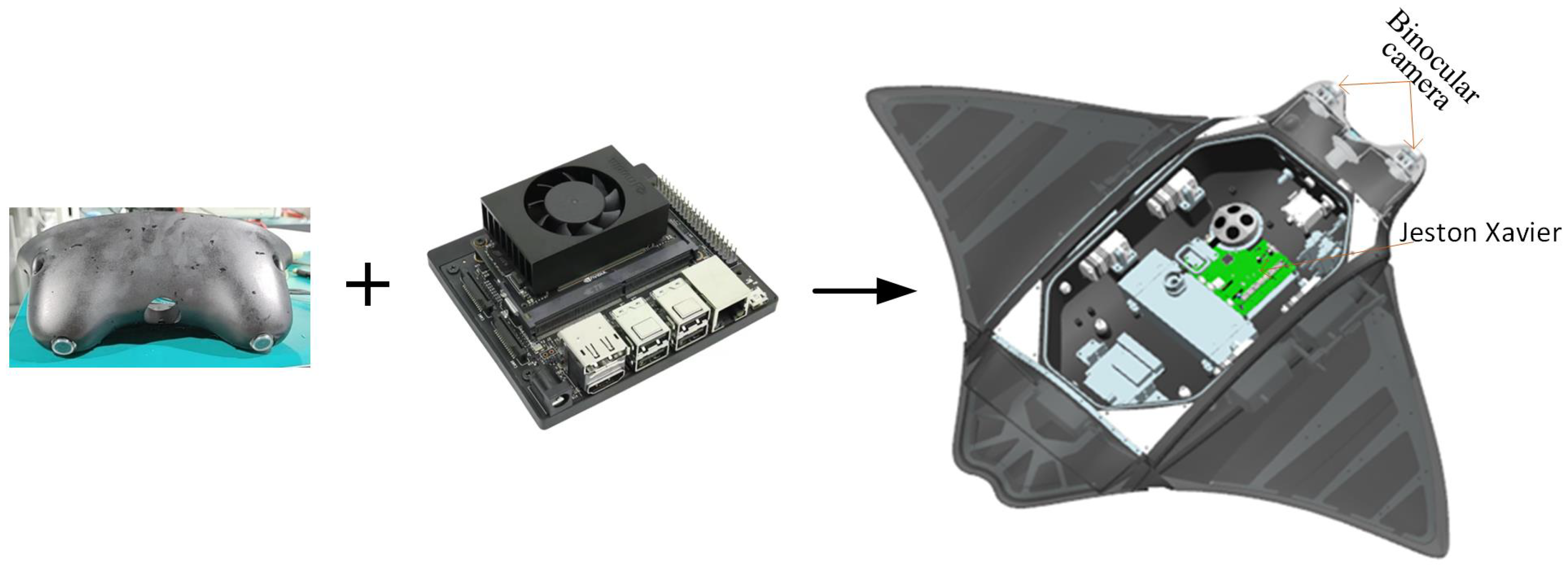
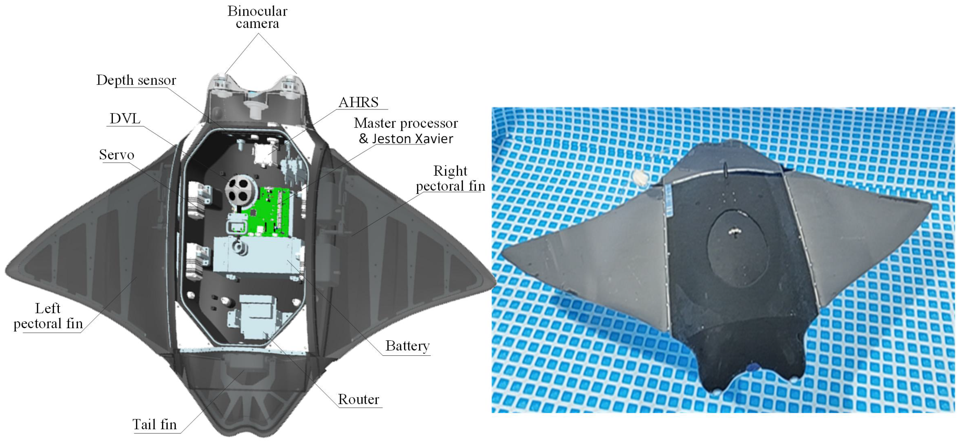
2.1. Description of the UBMRV

The UBMRV described in this paper has a wingspan of 1.2 m, a body length of 0.8 m, a weight of 20 kg, and a maximum flapping speed of 2 knots. The prototype and internal module layout of the UBMRV developed by the team are shown in Figure 3.

The prototype head was equipped with two camera modules. A Doppler velocity log (DVL) was placed on the abdomen. The interior of the prototype cabin contained modules such as an attitude and heading reference system (AHRS), router, depth sensor, main control board, and battery. The distributions of each module on the aircraft prototype are shown in Figure 3. The sensor data were sent to the main control processor through the serial port to realize the autonomous motion estimation of the UBMRV.

AHRS usually consists of a multi-axis gyroscope, multi-axis accelerometer, and magnetic compass. The data collected by these sensors were fused through a Kalman filter to give the vehicle three degrees of freedom of motion (yaw, pitch, and roll).

DVL uses the Doppler shift between the transmitted acoustic wave and the received bottom-reflected wave to measure the vehicle’s speed and accumulated range relative to the bottom. From the Doppler effect, DVL can calculate the speeds of the forward, right, and up axis.

The depth sensor was used to measure the depth information of the UBMRV. The vehicle implemented depth closed-loop control based on this measured depth information value. Two camera modules were used to measure the relative distance and bearing information of neighbors. The vehicle used the information to achieve formation control.

2.2. Description of Relative Positioning System Based on Binocular Camera

2.2.1. Object Detection Module

Deep learning object detection methods are divided into single-stage and two-stage detection methods, such as RCNN and faster-RCNN algorithms [17]. In this paper, the YOLO series of single-stage methods with fast calculation speeds were used to perform real-time detection of the UBMRV. Since there are few categories of objects detected in this study, the trained network model should be deployed on NVIDIA Jeston NX for real-time object detection. Therefore, this paper uses YOLOx-m with a relatively small model size as the basic algorithm for object detection.

The YOLOx network mainly includes components, such as input, backbone, neck, and head. On the network input side, YOLOx mainly adopts two data enhancement methods, Mosaic and Mixup. Backbone adopts the DarkNet53 and SPP layer architecture as the benchmark model algorithm. Basic feature extraction was performed on the input image information through a convolutional network, cross-stage partial network (CSPNet), batch normalization, and SiLU activation function. The neck layer uses the FPN feature pyramid upsampling and horizontal connection processes to achieve multi-scale feature fusion. The function of the head layer is to output the detection object result, including the object category, the predicted category’s confidence, and the object’s coordinates on the image. The YOLOx model has three detection heads with different feature scales and uses convolution operations on the feature maps of different scales to obtain the object output.

The head part of the YOLOx network adopts the decoupled head structure, which is divided into cls_output, reg_output, and obj_output. Where cls_output mainly predicts the categories of anchor points, reg_output predicts the coordinate information of the anchor point, and obj_output determines the positive and negative samples of the anchor point.

The loss of the YOLOx network consists of $L_{cls}$, $L_{reg}$, and $L_{obj}$. $L_{cls}$ represents the predicted category loss. $L_{reg}$ represents the regression loss of the predicted anchor point. $L_{obj}$ represents the confidence loss of the predicted anchor point. The loss function of YOLOx can be expressed as,

$$Loss=\frac{L_{cls}+\lambda L_{reg}+L_{obj}}{N_{pos}}$$

(1)

where $L_{cls}$ and $L_{obj}$ use binary cross-entropy loss and $L_{reg}$ uses IoU loss. $\lambda$ is the equilibrium coefficient of the regression loss, and $N_{pos}$ denotes the number of anchor points classified as positive samples. $L_{cls}$ and $L_{reg}$ only calculate the loss of positive samples, and $L_{obj}$ calculates the total losses of positive and negative samples.

2.2.2. Relative Distance and Bearing Estimation Module

In this study, the binocular camera was used to calculate the distance of the detected object. Two parallel cameras mounted on the head of the UBMRV were used to capture the imaging information of the moving object. We input the collected image to the object detection module and output the target’s position information on the image. Within the bounding box, the ORB was used to realize the feature extraction and matching process. The relative distance and bearing information between the UBMRV were obtained using the principle of the binocular distance measurement.

The binocular distance measurement process can be divided into camera calibration, stereo rectification, feature matching, and disparity calculation. Due to unavoidable differences, such as mounting between the left and right cameras, the captured image will be distorted. Therefore, the first step is to obtain the distortion parameters of the camera through camera calibration. In this study, the ORB algorithm was used to extract and match the features in the object-bounding box of the left and right images. The main advantage of the ORB algorithm is that the calculation speed is fast and can meet real-time requirements. Finally, the disparity is calculated for the matching feature points of the left and right images, and the actual relative distance between the UBMRV is obtained by combining it with the camera’s intrinsic matrix.

The purpose of stereo rectification is to align the two imaging planes and align the pixels on each row, thereby reducing the search range of the feature-matching algorithm and reducing the complexity of the binocular distance estimation. The object detection algorithm based on YOLOx can obtain the position coordinates of the target on the image, which are relative to the image coordinates system. To achieve relative positioning between robots, it is necessary to match the features extracted from the left and right images and use the principle of stereo ranging to obtain the position coordinates of the target in the actual coordinate system.

The world coordinate system has $C_1$ and $C_2$ cameras. The pixel point projected by the three-dimensional point P on the camera is $p_1$, $p_2$. We used triangulation to obtain the coordinates of point P in the three-dimensional space. First, we completed the stereo rectification operation to align the polar lines of the left and right images in the horizontal direction. After stereo rectification, the two images only had disparity in the horizontal direction. Thus, the stereo-matching problem was reduced from two-dimensional to one-dimensional, which improved the matching speed.

The stereo rectification of the binocular camera mainly solves the homography transformation matrix corresponding to the left and right cameras, according to the principle of camera projection, if there is a point in space P. The coordinates in the world coordinate system are ${[X_w,Y_w,Z_w]}^T$; the coordinates in the camera coordinate system are ${[X_c,Y_c,Z_c]}^T$. After the projection transformation, the coordinates in the imaging plane are ${[x,y]}^T$. The coordinates in the pixel coordinate system are ${[u,v]}^T$. Figure 4 shows the camera projection transformation relationship.

The rotation matrix R and displacement vector T represent the mapping relationship of points in the world coordinate system and camera coordinate system.

$$P_w=R\times P_c+T$$

(2)

where $T=C$ and C are the coordinates of the origin of the camera coordinate system in the world coordinate system. The relationship between the left camera and the right camera is obtained from the camera projection relationship,

$${\lambda }_L\left[\begin{array}{c}{u}_L\\ v_L\\ 1\end{array}\right]=K_L{R}_L^{-1}\left(\left[\begin{array}{c}{X}_w\\ Y_w\\ Z_w\end{array}\right]-C_L\right)$$

(3)

where $\lambda$ is the scaling factor. K is the intrinsic matrix of the cameras. R and C are the rotation matrices and translation vectors of the camera, respectively. The projection relationship expression of the right camera can be obtained in the same way.

Since the two virtual cameras are identical, they have the same external parameter R and intrinsic matrix K. The projection relationship of the space point P on the virtual plane is

$${\widehat{\lambda }}_L\left[\begin{array}{c}{\widehat{u}}_L\\ {\widehat{v}}_L\\ 1\end{array}\right]={\widehat{K}}_L{\widehat{R}}_L^{-1}\left(\left[\begin{array}{c}{X}_w\\ Y_w\\ Z_w\end{array}\right]-C_L\right)$$

(4)

The projection relationship between the original camera and the virtual camera is compared to obtain the homography matrix from the original image of the left camera to the new virtual image.

$$\begin{array}{cc}\hfill \left[\begin{array}{c}{\widehat{u}}_L\\ {\widehat{v}}_L\\ 1\end{array}\right]& =\frac{{\lambda }_L}{{\widehat{\lambda }}_L}\widehat{K}{\widehat{R}}^{-1}{R}_L{K}_L^{-1}\left[\begin{array}{c}{u}_L\\ v_L\\ 1\end{array}\right]\hfill \\ \hfill & =H_L\left[\begin{array}{c}{u}_L\\ v_L\\ 1\end{array}\right]\hfill \end{array}$$

(5)

Similarly, the homography matrix of the right camera can be obtained. The image after stereo correction is shown in Figure 5.

3. Design of the UBMRV Positioning Algorithm Based on Improved YOLOx

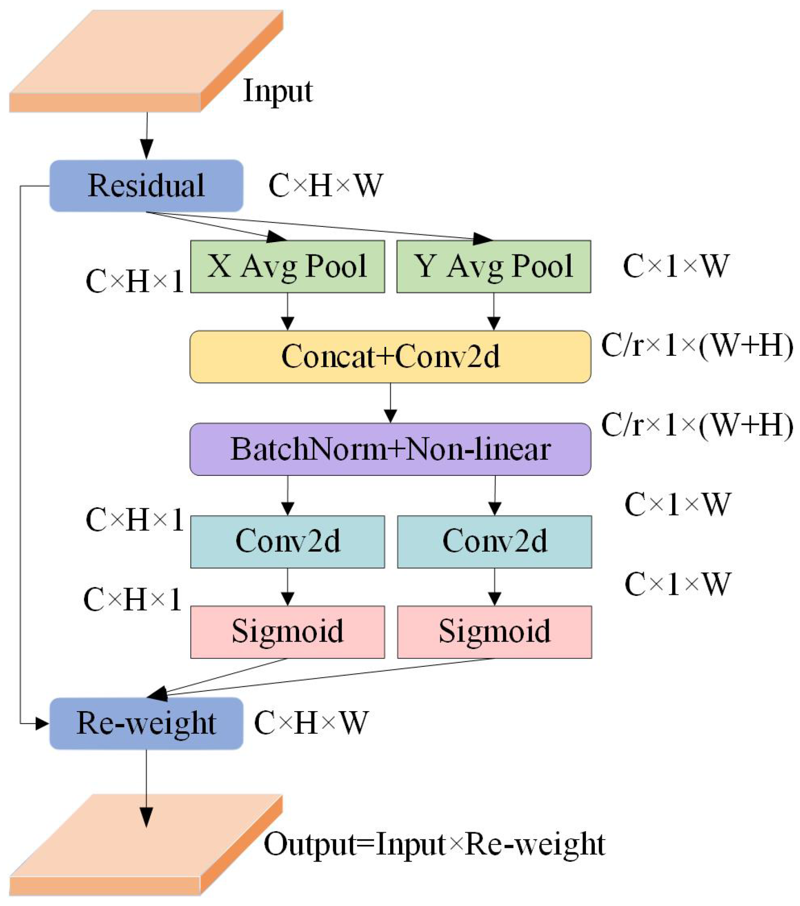
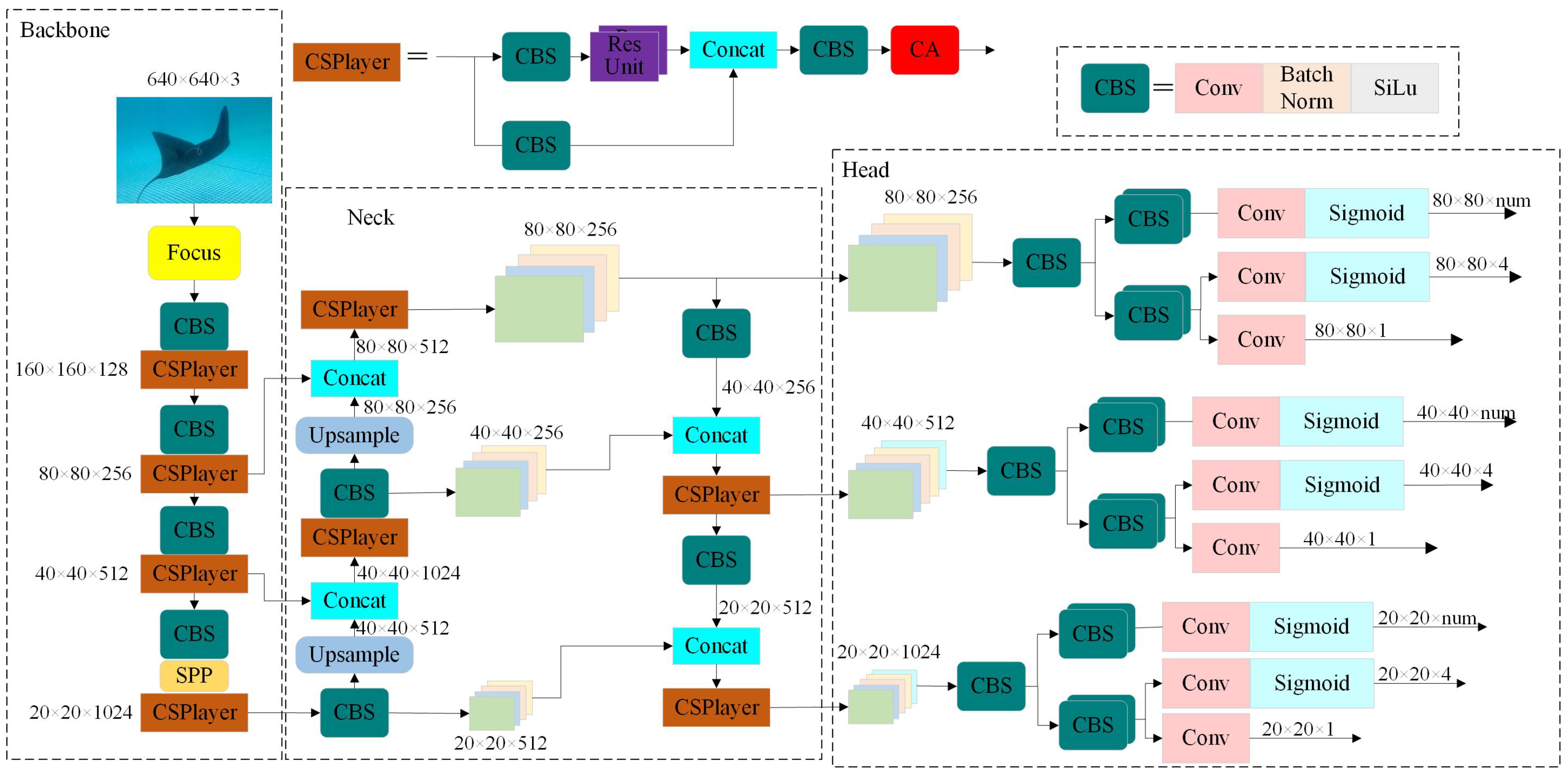
3.1. Improved YOLOx Network Design

In order to improve the detection precision of the UBMRV in small samples, the original YOLOx network structure was improved in this study. The coordinate attention(CA) module [18] was added to the YOLOx network structure to improve the detection precision of the model. The essence of the attention mechanism is to assign different weights to the positions of pixels of different feature layers and different channels in the object detection network model through the function of external data or the internal correlation of data features so that the model can locate the information of interest and suppress the useless information. The coordinate attention mechanism embeds location information into channel attention, enabling the network to capture large-region relationships and model the dependencies between different channel information in vision tasks. At the same time, the attention mechanism module does not generate much computational overhead.

Compared with other attention mechanism modules, coordinate attention does not lose the location information of features when performing global pooling operations. This is important for object detection tasks that require location information output. The network structure of the coordinate attention module is shown in Figure 6. The attention mechanism employs two one-dimensional global pooling operations to aggregate the horizontal and vertical input features into two independent orientation-aware feature maps. These two feature maps with specific orientation information are encoded into two attention maps. Each attention map captures the channel correlations of the input feature maps along the spatial direction, assigning different weights to the input feature maps to improve the representation of the region of interest.

For input X, each channel is first coded in the horizontal and vertical directions using pooled cores with dimensions $(H,1)$ and $(1,W)$. The output of the c channel with height h can be expressed as

$$z_c^w\left(h\right)=\frac{1}{W}\sum _{1\le i\le W}{x}_c(h,i)$$

(6)

Similarly, the output of the c channel with width w is expressed as

$$z_c^w\left(w\right)=\frac{1}{H}\sum _{1\le i\le H}{x}_c(j,w)$$

(7)

Concatenation of the transformation along two directions obtains a pair of directional awareness attention maps, then use a shared 1 × 1 convolution to perform the $F_1$ transformation, which is expressed as

$$f=\sigma \left(F_1\left([z^h,z^w]\right)\right)$$

(8)

Among them, $\sigma$ represents a sigmoid function. Further, f is divided into two separate tensors $f_h$, $f_w$, along the spatial dimension. Two 1 × 1 convolutions are used to transform the characteristic graph $f_h$, $f_w$ to the same number of channels as input X.

$$\begin{array}{c}{g}^h=\sigma \left(F_h\left(f^h\right)\right)\\ g^w=\sigma \left(F_w\left(f^w\right)\right)\end{array}$$

(9)

Using $g^h$,$g^w$ as attention weights, the output of the CA module can be obtained as

$$y_c(i,j)=x_c(i,j)\times g_c^h\left(i\right)\times g_c^w\left(j\right)$$

(10)

In this study, the CA module is added to the CSPlayer module. The network structure after adding the CA module is shown in Figure 7. The overall network structure is divided into CSPDarknet, FPN, and head.

The CA module is mainly added to the main feature extraction part of YOLOx to improve the precision of the feature extraction of the input image by the network. The input images first enter the focus structure, the width and height data of the images are concentrated on the channel information to complete the channel expansion process. Then feature extraction is conducted by using the convolutional layer and the CSPlayer layer. The extracted features are called the feature sets of the input images. After the main feature extractions of the input images are complete, three feature layers with scales of 80 × 80, 40 × 40, and 20 × 20 are the output. These three feature layers are called effective feature layers and serve as the input for the next step of network construction.

The feature fusion of the three effective feature layers are performed through the FPN structure. The purpose of feature fusion is to combine feature information of different scales to achieve further feature extraction.

After the input image is extracted through the backbone feature and the FPN structure, three effective feature layers with width, height, and many channels are output. Each feature layer can obtain three prediction results, namely regression parameters, positive and negative sample prediction, and category prediction.

We used the binocular camera on the prototype to acquire a full range of images of the UBMRV in different lighting environments and orientations. More than 10,000 images were collected. We selected 8700 images for category annotation and bounding box annotation to create the dataset for network training. We divided the produced dataset into the training set, testing set, and validation set according to the ratio of 8:1:1.

Moreover, the original YOLOx was used to compare with the improved YOLOx. The training was performed using the same platform. The training Epoch was set to 200; the final training results are shown in

Table 1. Comparison of original YOLOx and improved YOLOx.

Model	Precision	Training Time (Hour)	Detection Rate (fps)
YOLOx	98.98%	2.0	58
YOLOx+CA	99.32%	2.3	56

.

As can be seen from the training results in the table, the addition of the CA module to the original YOLOx model improves the precision of object detection. However, the training duration becomes slightly longer due to the increased complexity of the model. Adding the CA module increases the weights generated by the network training. Therefore, the speed of detecting objects was slightly reduced. Since this study only recognizes one class of the UBMRV, the precision of detection is high.

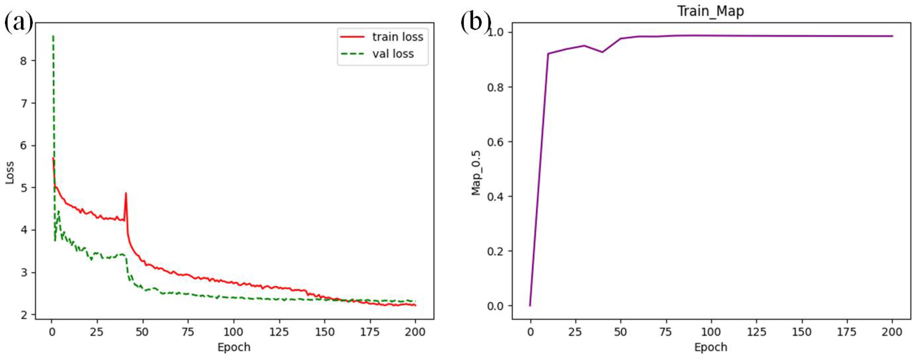
3.2. Model Training and Testing

We trained the proposed network model on a GPU with NVIDIA GeForce RTX3090, a CPU with Intel Core i9-10980XE, and an Ubuntu system. After preparing the dataset and the network model structure needed for network training. We performed the training parameter setting and input the produced dataset into the network for training and validation.

The official YOLOx network pre-training model was used as the weight model file for training. To improve the model’s generalizability, we performed freeze training on the model. The freeze training epoch was set to 40, and the total training process was set to 200 epochs. The training process uses small batch stochastic gradient descent as the optimizer. The learning rate peak is set to 0.01. The cosine learning rate decay strategy is used, and the momentum is set to 0.937. We use Mixup and Mosaic data augmentation methods. Data augmentation is stopped in the last 15 epochs to improve the model precision.

Figure 8a shows the loss changes in the training and validation sets during the training of the network. The figure shows that the loss value decreases more at the beginning of the training phase, indicating that the network learning rate is set appropriately and undergoes the gradient descent process. As the training epoch increases, the loss curves of both the training and validation sets show a decreasing trend. Although the loss values jumped slightly during the training process, the losses eventually stabilized, and the losses changed slowly after stabilization. After 150 epochs, the loss of the training set reached 2.2, and the loss of the validation set was 2.25.

Figure 8b shows the change curve of the object detection accuracy of the network when the IoU was set to 0.5 during the network training. mAP was used to measure the accuracy of object detection, i.e., the average value of AP. Higher values of mAP indicate better detection of the object detection model on a given dataset. mAP_0.5 represents the AP of each image category calculated and averaged over all image categories when IoU is set to 0.5. Since the number of categories detected in this study was 1, the AP values obtained were the same as the mAP values. It can be seen from the figure that when the network was trained to 100 epochs, the mAP of this network reached 99.0%, and the detection accuracy of the object tended to be stable.

Figure 9 plots the prediction results of the network on the test dataset. Figure 9a represents the precision recall curve plot when the IoU was 0.5. Figure 9b shows the F1 value change curve for different IoU thresholds. Figure 9c shows the precision change curve for different IoU thresholds. Figure 9d shows the recall change curve for different IoU thresholds. AP measures how well the trained model can detect the category of interest. The area enclosed by the PR curve is the AP value of the network object detection. From the PR curve in the figure, we see that the network achieves 99.0% AP for detecting the UBMRV category on this dataset.

Precision represents the proportion of positive predictions that are positive. Precision can be considered the ability of the model to find the correct data. The F1 is the summed average of Precision and Recall, and is a composite evaluation metric of Precision and Recall. It is used to avoid a single extreme value of Precision or Recall and is a comprehensive indicator of the whole [19]. The calculation formula of each index is shown in Equation (11):

$$\begin{array}{cc}\hfill Precision& =\frac{TP}{TP+FP}\hfill \\ \hfill Recall& =\frac{TP}{TP+FN}\hfill \\ \hfill F_1& =2\times \frac{Precision\times Recall}{Precision+Recall}\hfill \end{array}$$

(11)

$TP$ indicates that if the prediction is positive and the actual is positive, then the prediction is correct. $FP$ means that if the prediction is positive and the actual is negative, then the prediction is wrong. $FN$ means that if the prediction is negative and the actual is positive, the prediction is wrong. From the prediction results graph, it can be seen that when the IoU threshold is 0.5, the predicted precision is 99.32%, and recall is 98.98% on the data set of this study. Since the values of both precision and recall are large, this study calculated the $F_1$ value when the IoU threshold was 0.5 and obtained its value of 0.99. The prediction results show that the network model has a good object detection performance on the test dataset.

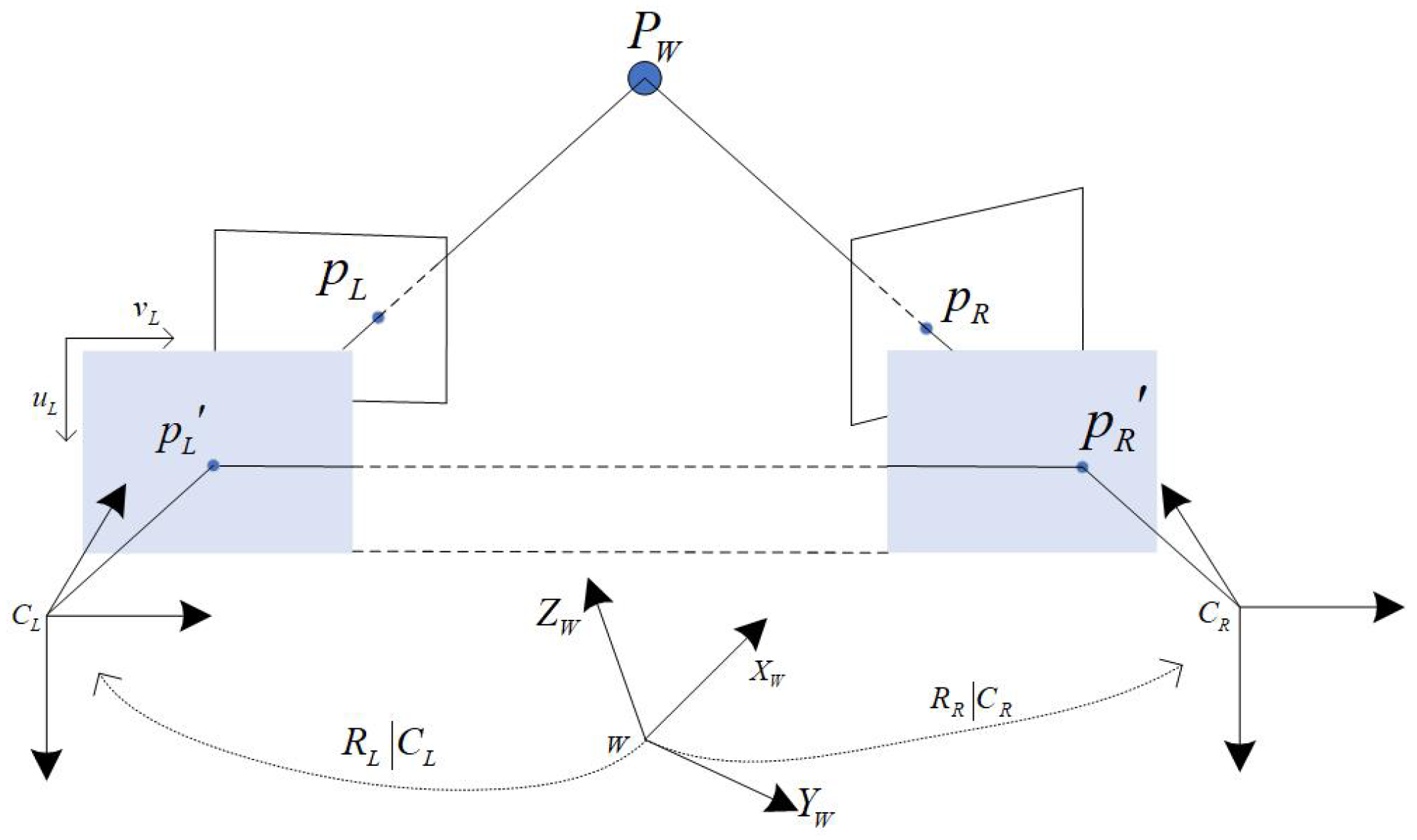
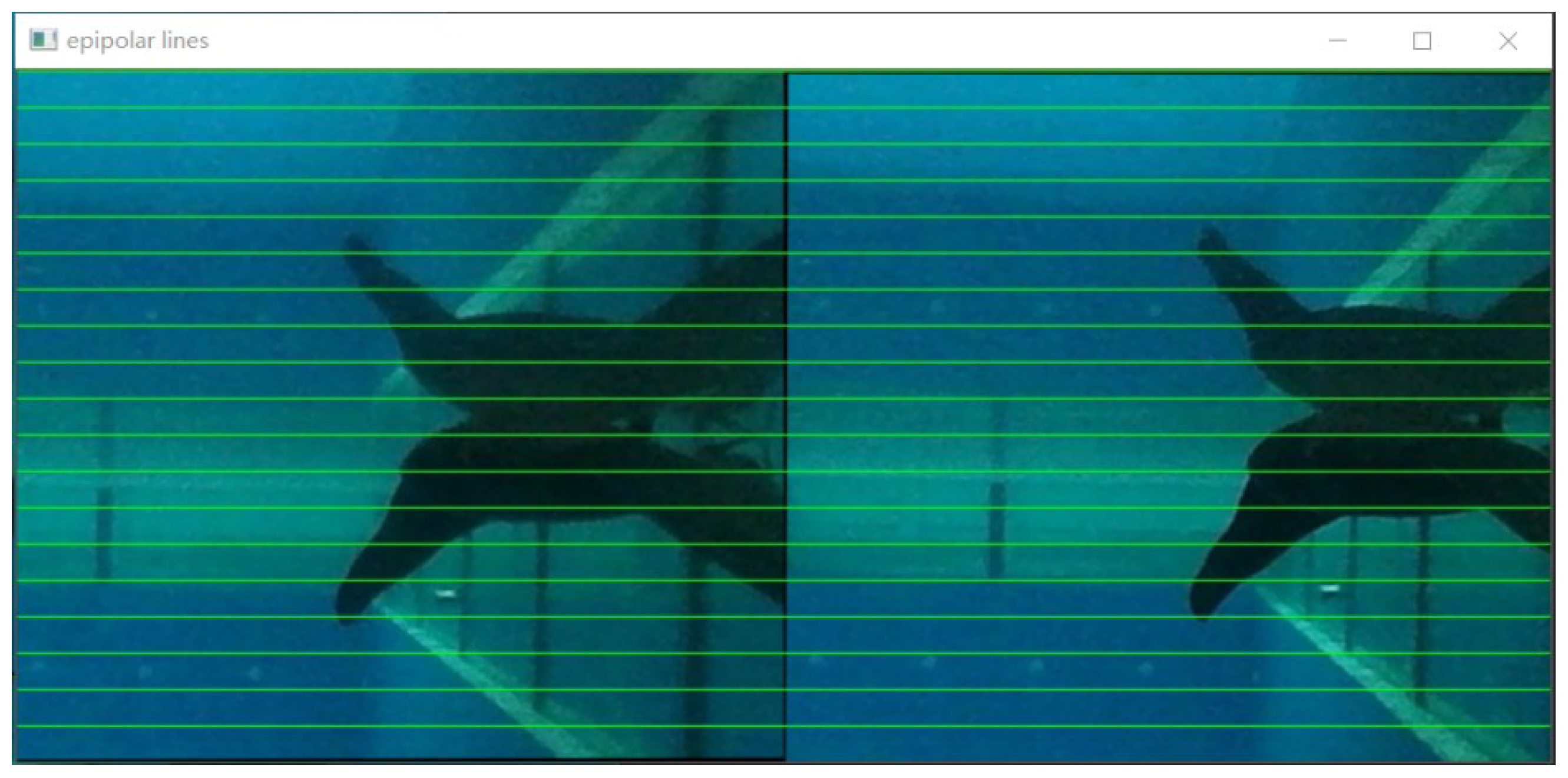
3.3. Relative Distance and Bearing Estimation Based on Binocular Camera

It is well known that the most important parts of binocular distance measurements are matching features. In this study, the ORB algorithm was used for feature extraction and matching under the requirement of real-time system consideration.

First, the position information of the UBMRV on the image was obtained from the image captured by the binocular camera after the object detection module. The coordinates of the predicted bounding box on the left image are defined as $(x{1}_l,y{1}_l)$ for the upper left corner and $(x{2}_l,y{2}_l)$ for the lower right corner. Similarly, the coordinates of the upper left corner $(x{1}_r,y{1}_r)$ and lower right corner $(x{2}_r,y{2}_r)$ of the bounding box on the right image can be obtained. The matching points corresponding to the left image are extracted from the bounding box on the right image. Firstly, the overlap degree was calculated for the bounding box of the left and right figure, as in Equation (12).

$$p=\frac{S[max(x{1}_l,x{1}_r),max(y{1}_l,y{1}_r),min(x{2}_l,x{2}_r),min(y{2}_l,y{2}_r)]}{max\{S[(x{2}_l-x{1}_l)\times (y{2}_l-y{1}_l)],S[(x{2}_r-x{1}_r)\times (y{2}_r-y{1}_r)]\}}$$

(12)

where S represents the calculated area.

If the overlap within the left and right two bounding boxes is large, then the left and right images are cut according to the coordinates of the detected object on the image. Thus, the region for ORB feature extraction is obtained. Otherwise, no more feature extraction is performed.

After obtaining the region for ORB feature extraction, the feature points are extracted using the oriented fast algorithm [20] only within the bounding box. After the object key points are extracted, their descriptors are calculated for each point. Then the features of the left and right images are matched, and the pixel location information of the matched features is obtained. Finally, the disparity and depth values of the object are calculated from the pixel location information of the left and right images.

FAST is known for its rapidity, and it mainly determines whether a pixel is a corner point by detecting the local pixel where the grayscale changes significantly. ORB improves on the shortcomings of the FAST algorithm in terms of the uncertainty of the number of feature points and the fact that features are not scalable and directional [21]. First, by specifying the final number of feature points to be extracted N, the Harris response value R is calculated separately for FAST corner points, as shown by Equation (13).

$$\begin{array}{cc}\hfill R& =det\left(M\right)-k{\left(trace\left(M\right)\right)}^2\hfill \\ \hfill M& =\sum _{x,y}w(x,y)\left[\begin{array}{cc}{I}_x^2& I_x{I}_y\\ I_x{I}_y& I_y^2\end{array}\right]\hfill \\ \hfill det\left(M\right)& ={\lambda }_1{\lambda }_2\hfill \\ \hfill trace\left(M\right)& ={\lambda }_1+{\lambda }_2\hfill \end{array}$$

(13)

where ${\lambda }_1$ and ${\lambda }_2$ are the eigenvalues of the matrix M. (x,y) is the coordinate of the corresponding pixel in the window, and $w(x,y)$ is the window function. $I_x$ and $I_y$ represent the gradient coordinates of each pixel.

The Harris response value is calculated by solving the eigenvalues of the matrix M. Finally, the N feature points with the largest response values are selected as the final feature point set.

ORB uses the grayscale center of mass in solving the rotation of features and the center of mass is the center with the weight of the grayscale value of the image block. In a small image block D, the moments of the image block are defined as,

$$m_{pq}=\sum _{x,y\in D}{x}^p{y}^{q}I(x,y);p=\{0,1\};q=\{0,1\}$$

(14)

From the moments of the image block, the center of mass of the image block is

$$C=\left(\frac{m_{10}}{m_{00}},\frac{m_{01}}{m_{00}}\right)$$

(15)

Connecting the geometric center O and the center of mass C of the image block yields the vector $\overrightarrow{OC}$, and the direction of the feature point is

$$\theta =arctan\frac{m_{01}}{m_{00}}$$

(16)

At this point, the ORB feature extraction process is completed.

After extracting the feature points, the descriptor is calculated for each point. ORB uses the BRIEF feature description, and the BRIEF description is a binary descriptor. This descriptor uses a random point selection method, making the computation faster. The use of binary representation is easy to store and is suitable for real-time image matching.

This study uses a violent matching method [22] for feature matching between the left and right images. The descriptor distance represents the degree of similarity between the two features. The distances between the feature point descriptors in the left image and right image are measured, and the measured distances are ranked. The nearest distance is finally taken as the matching point between the features.

In this study, 20 points are taken for feature matching for the left and right graphs, respectively. Since the binocular camera has completed distortion rectification and stereo rectification, i.e., the two images (non-co-planar row-aligned) are corrected to be co-planar row-aligned, as shown in Figure 4. Therefore, the distance is directly calculated for the matched feature points using the binocular distance measurement principle, as shown in Figure 10.

The distance between the optical centers of the two cameras is called the baseline (noted as b), and parameter b is known after the camera mounting position is determined. If point P exists in space, the imaging on the left and right cameras are noted as $P\_L$ and $P\_R$. After aberration and stereo rectification, only the image on the x-axis is displaced. Therefore, the position of P on the image plane also differs only on the x-axis, corresponding to the u-axis of the pixel coordinates. Let the coordinates of $P\_L$ on the left image be $x\_l$ and on the right image be $x\_r$. The geometric relationship is shown in Figure 10. According to the triangle similarity, we have

$$\frac{z}{f}=\frac{x}{x_l}=\frac{x-b}{x_r}=\frac{y}{y_l}=\frac{y}{y_r}$$

(17)

Then, we have,

$$x=\frac{b\times x_l}{x_l-x_r};z=\frac{b\times f}{x_l-x_r};y=\frac{b\times y_l}{x_l-x_r}$$

(18)

and,

$$z=\frac{b\times f}{d};x=\frac{z\times x_l}{f};y=\frac{z\times y_l}{f}$$

(19)

where $d=x\_l-x\_r$ is the difference between the left camera and right camera pixel coordinates, called disparity. f is the camera’s focal length, and b is the baseline of the binocular camera. This gives the position coordinates of the feature points on the image under the camera coordinate system as $(x,y,z)$, and the relative distance is $dis=\sqrt{x^2+y^2+z^2}$.

The camera coordinate system is established with the left camera optical center of the binocular camera as the origin. Then the bearing of the feature points on the image for the camera can be expressed as

$$\alpha =arctan\frac{x}{z};\beta =arctan\frac{y}{z}$$

(20)

We arranged the distance values calculated in the bounding box in order and took the middle distance value as the final UBMRV relative distance and bearing.

4. Experiment and Analysis

The UBMRV conducted experiments on underwater object detection and relative distance estimation in a pool that was 732 cm × 366 cm × 132 cm. The effectiveness and feasibility of the method proposed in this study were verified. At the beginning of the experiment, the binocular camera needs to be calibrated in the underwater environment to obtain the calibration parameters of the camera. Then, the distortion correction and stereo rectification are applied to the binocular camera to prepare for binocular distance estimation.

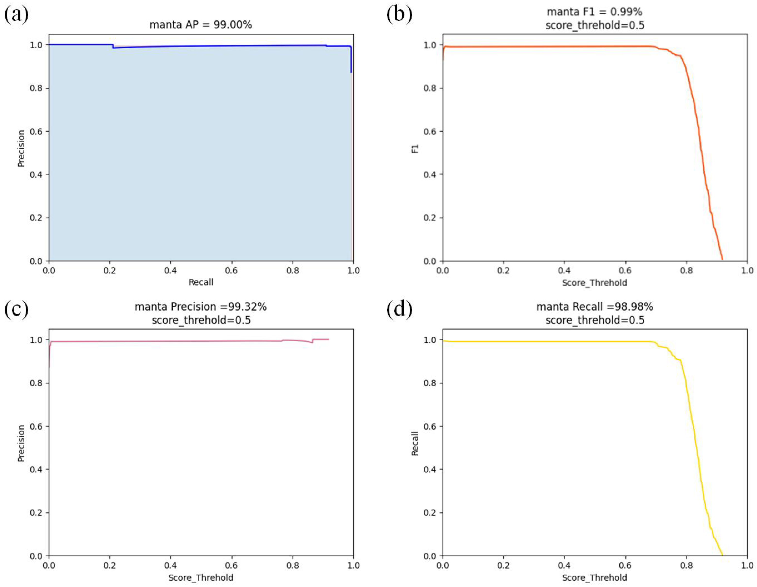
4.1. The UBMRV Object Detection Experiment

We used the binocular camera to acquire images of the UBMRV under different angles and lighting environments and made the dataset needed for network training. Then the network was trained using the object detection algorithm proposed in this paper, and the trained weight model file was obtained.

In order to realize the engineering application of the algorithm, the trained algorithm was deployed on the NVIDIA Jeston NX IPC of the prototype platform in this study. Since the whole algorithm framework was implemented under the PyTorch architecture, we used TensorRT to accelerate the deployment of the model in order to improve its inference speed. This study used Docker images to port the deployed environment. The algorithm environment configured with Docker images can be separated from the original system environment of the IPC. Using the Docker image approach can improve the efficiency of deploying the algorithm environment and make it easier to implement engineering applications.

After deploying the algorithm on the prototype, two UBMRVs equipped with binocular cameras were distributed in the pool in front and back positions. The rear prototype detects the front prototype, and the results of partial UBMRV object detection are obtained as shown in Figure 11.

We used the camera mounted on the head of the prototype to detect the neighboring UBMRV. From the underwater experiments, the visible distance of the camera was 5 m. When the distance between neighboring UBMRVs exceeds 5 m, the rear UBMRV cannot see the object ahead. We performed 20 detections of neighboring UBMRVs at 1 m, 1.5 m, 2 m, 2.5 m, 3 m, 3.5 m, 4 m, and 5 m, respectively. The number of successful detections of the neighboring objects was also counted and defined as the effective detection rate. The detection results are shown in

Table 2. Object detection results.

Relative Distance	1 m	1.5 m	2 m	2.5 m	3 m	3.5 m	4 m	5 m
Effective detection rate	100%	100%	100%	100%	95%	80%	70%	40%
Averaged effective detection rate	85.625%
Influence speed	25 fps

. When the relative distance between UBMRVs was close, at 1–3 m, the neighbors were detected using the algorithm proposed in this paper, and the effective detection rate reached more than 90%. When the relative distance between UBMRVs and neighbors was farther, 3 m or more, the effective detection rate of the object was 70–80%. The probability of successful detection of the object was low. Finally, we calculated the average probability of the successful detection of a neighboring object within the visible distance of the camera as 85.6%. The detection speed of the proposed algorithm deployed on NVIDIA Jeston NX can reach 25 fps, which meets the real-time requirements needed for subsequent control.

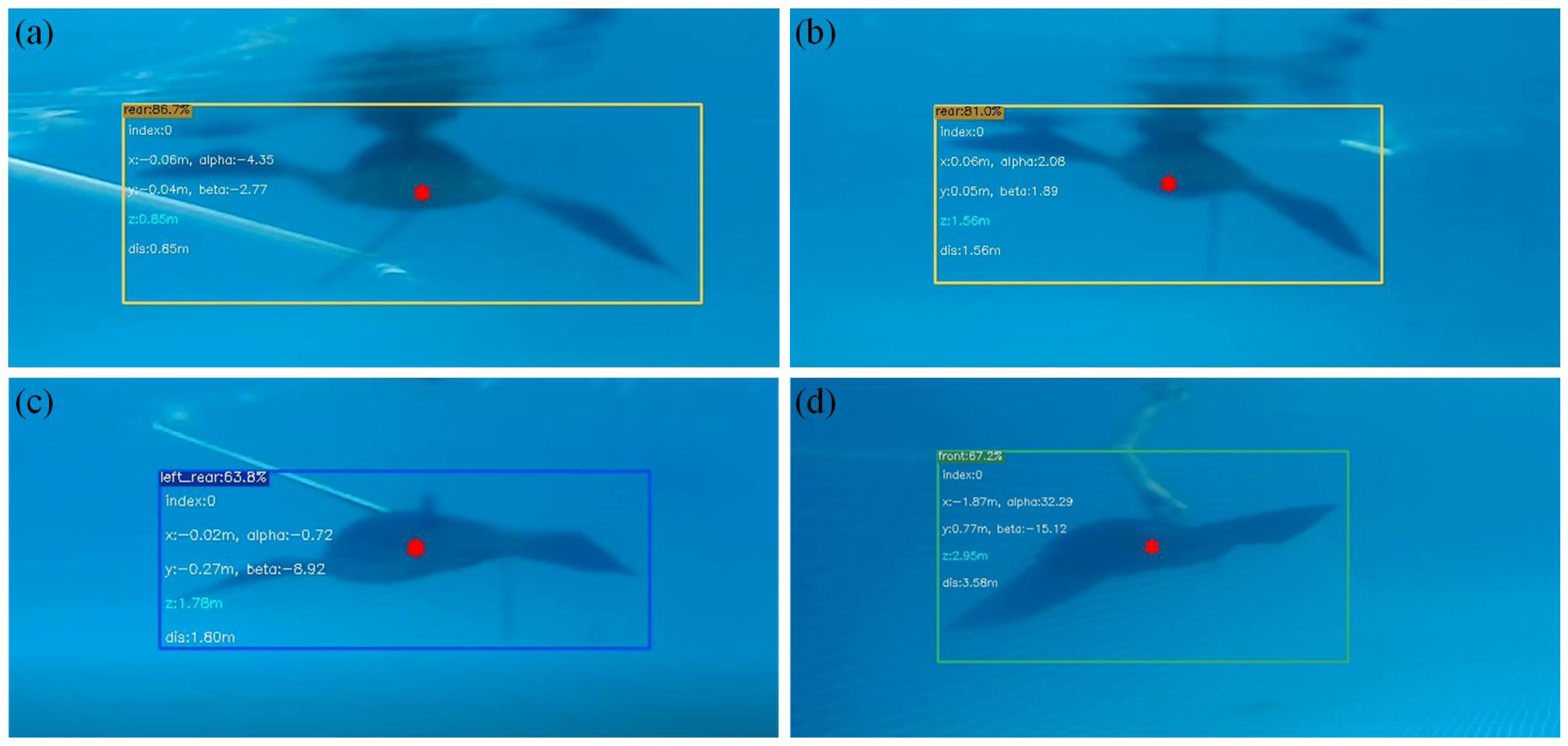
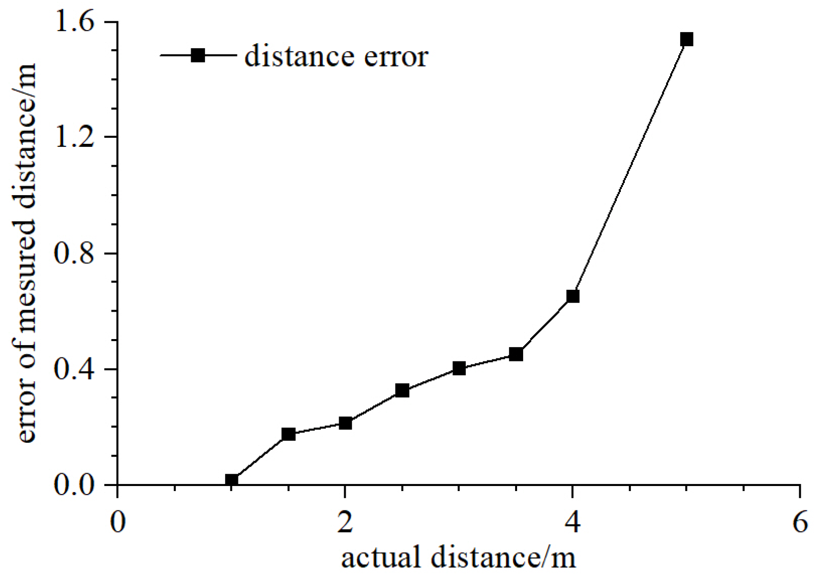
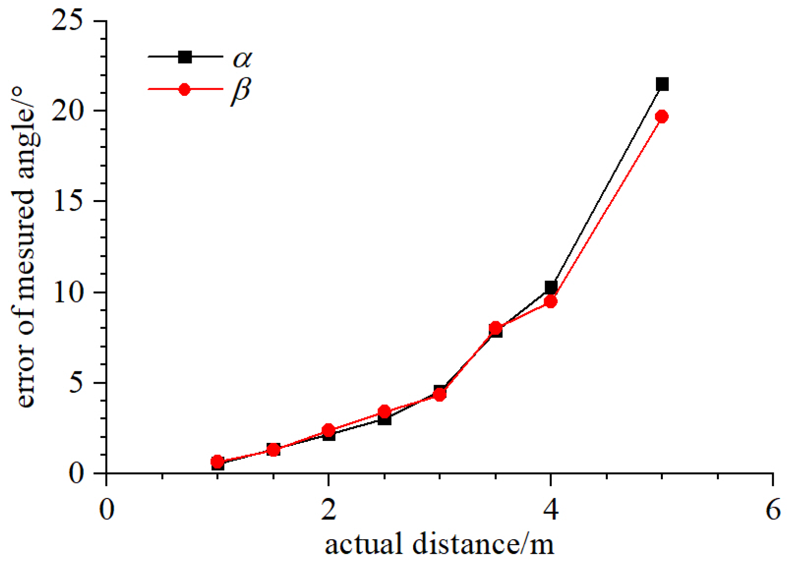
4.2. Experiment on Relative Distance and Bearing Estimation

We used the ORB method to extract features from the left and right images after completing the object detection. The biggest advantage of the ORB algorithm was the fast computation speed. This study performed feature extraction and matching only in the object detection area frame after obtaining the matching results to the left and right images. The binocular distance measurement principle was used to calculate the relative distance and bearing of the object. Finally, we show the final results on the left image. The experimental results of the relative distance and bearing estimation based on object detection are shown in Figure 12.

Similarly, we conducted 20 experiments on distance estimations at 1 m, 1.5 m, 2 m, 2.5 m, 3 m, 3.5 m, 4 m, and 5 m, respectively. The error between the measured distance and the real distance value was calculated. The average value of the 20-times measured distance error was taken as an evaluation index of the distance error. The distance error is relative to the length of the UBMRV platform. The experimental results of relative distance estimation are shown in

Table 3. Results of relative distance estimation.

Relative Distance	1 m	1.5 m	2 m	2.5 m	3 m	3.5 m	4 m	5 m
Distance error	0.0164 m	0.1751 m	0.2132 m	0.3274 m	0.4039 m	0.4518 m	0.6512 m	1.5386 m
Total time	0.2 s–0.25 s

and Figure 13.

We conduct 20 experiments of bearing estimation in each of the 8 positions as shown in

Table 4. Results of relative bearing estimation.

Actual Location (cm)	(20,30,100)	(−35,40,145)	(40,15,200)	(40,−100,230)	(100,60,280)
bearing error $\alpha {(}^{°})$	0.532	1.320	2.156	3.047	4.539
bearing error $\beta {(}^{°})$	0.635	1.286	2.381	3.408	4.328
Actual location (cm)	(−240,−15,270)	(400,20,150)	(250,10,430)
bearing error $\alpha {(}^{°})$	7.863	10.267	21.485
bearing error $\beta {(}^{°})$	8.034	9.485	19.690

. The angle with the x-axis direction was taken as $\alpha$ and the angle with the y-axis direction was taken as $\beta$. The error between the measured and true values was calculated, and the average value of the angular error of the 20 measurements was taken as the index of the angular error estimation. The experimental results of the relative bearing estimations are shown in Figure 14.

From the above distance and bearing error graphs, it can be seen that when the relative distance between targets was close, there was high accuracy regardless of whether object detection or distance and bearing estimation were performed. When the distance between objects was 1–3 m, the estimated distance error was around 0.3 m. The estimated angle error was around 4°. When the distance between objects was larger, the error changed more. From the experimental results, the binocular localization system proposed in this paper has good results in the case of close distance. The experimental error is relatively large at 3–5 m. The operation speed of the algorithm deployed on the IPC is 5 fps, which can meet the system’s real-time requirements.

5. Conclusions

In order to solve the relative positioning problem of the UBMRV cluster, this paper proposes a relative positioning method based on an object detection algorithm and binocular vision. The engineering realization of the UBMRV cluster can promote the completion of complex tasks, such as large-scale sea area monitoring and multi-task coordination, and relative positioning technology is one of the key technologies for realizing cluster formation. Therefore, this paper used a binocular camera to obtain the neighbor’s distance and bearing information to realize the relative positioning. We adopted an improved object detection algorithm to detect the neighbor’s UBMRV directly. From the experimental results, the improved object detection algorithm has higher precision. Then, this study used the ORB algorithm to extract and match features in the bounding box. This method reduces the computational burden of binocular matching. It can be concluded from the pool experiment that when the actual distance between neighbors is 1–3 m, both the object detection and relative distance estimation have high accuracy. When the actual distance is far, the positioning accuracy is poor, and even “invisible” occurs. This paper completes the design of the UBMRV cluster relative positioning system and deploys the proposed algorithm on the prototype for pool experiments. The algorithm’s running time is 0.2–0.25 s, which can meet the real-time requirements of the system.

To further improve the current research work—since the motion of UBMRV is divided into different poses—the motion poses of neighbors can be estimated through visual perception, thereby improving the formation positioning error. The ultimate goal is to realize the engineering application of the UBMRV formation.

References

1. Yuh, J. Design and control of autonomous underwater robots: A survey. Auton. Robot. 2000, 8, 7–24. [Google Scholar] [CrossRef]
2. Alam, K.; Ray, T.; Anavatti, S.G. Design optimization of an unmanned underwater vehicle using low-and high-fidelity models. IEEE Trans. Syst. Man, Cybern. Syst. 2015, 47, 2794–2808. [Google Scholar] [CrossRef]
3. Huang, Q.; Zhang, D.; Pan, G. Computational model construction and analysis of the hydrodynamics of a Rhinoptera Javanica. IEEE Access 2020, 8, 30410–30420. [Google Scholar] [CrossRef]
4. He, J.; Cao, Y.; Huang, Q.; Cao, Y.; Tu, C.; Pan, G. A New Type of Bionic Manta Ray Robot. In Proceedings of the IEEE Global Oceans 2020: Singapore–US Gulf Coast, Biloxi, MS, USA, 5–30 October 2020; pp. 1–6. [Google Scholar]
5. Cao, Y.; Ma, S.; Xie, Y.; Hao, Y.; Zhang, D.; He, Y.; Cao, Y. Parameter Optimization of CPG Network Based on PSO for Manta Ray Robot. In Proceedings of the International Conference on Autonomous Unmanned Systems, Changsha, China, 24–26 September 2021; pp. 3062–3072. [Google Scholar]
6. Ryuh, Y.S.; Yang, G.H.; Liu, J.; Hu, H. A school of robotic fish for mariculture monitoring in the sea coast. J. Bionic Eng. 2015, 12, 37–46. [Google Scholar] [CrossRef]
7. Chen, Y.L.; Ma, X.W.; Bai, G.Q.; Sha, Y.; Liu, J. Multi-autonomous underwater vehicle formation control and cluster search using a fusion control strategy at complex underwater environment. Ocean Eng. 2020, 216, 108048. [Google Scholar] [CrossRef]
8. Redmon, J.; Divvala, S.; Girshick, R.; Farhadi, A. You only look once: Unified, real-time object detection. In Proceedings of the IEEE Conference on Computer Vision and Pattern Recognition, Las Vegas, NV, USA, 27–30 June 2016; pp. 779–788. [Google Scholar]
9. Redmon, J.; Farhadi, A. YOLO9000: Better, faster, stronger. In Proceedings of the IEEE Conference on Computer Vision and Pattern Recognition, Honolulu, HI, USA, 21–26 July 2017; pp. 7263–7271. [Google Scholar]
10. Jiang, P.; Ergu, D.; Liu, F.; Cai, Y.; Ma, B. A Review of Yolo algorithm developments. Procedia Comput. Sci. 2022, 199, 1066–1073. [Google Scholar] [CrossRef]
11. Zhang, S.; Li, J.; Yang, C.; Yang, Y.; Hu, X. Vision-based UAV Positioning Method Assisted by Relative Attitude Classification. In Proceedings of the 2020 5th International Conference on Mathematics and Artificial Intelligence, Chengdu, China, 10–13 April 2020; pp. 154–160. [Google Scholar]
12. Feng, J.; Yao, Y.; Wang, H.; Jin, H. Multi-AUV terminal guidance method based on underwater visual positioning. In Proceedings of the 2020 IEEE International Conference on Mechatronics and Automation (ICMA), Beijing, China, 13–16 October 2020; pp. 314–319. [Google Scholar]
13. Chi, W.; Zhang, W.; Gu, J.; Ren, H. A vision-based mobile robot localization method. In Proceedings of the 2013 IEEE International Conference on Robotics and Biomimetics (ROBIO), Shenzhen, China, 12–14 December 2013; pp. 2703–2708. [Google Scholar]
14. Xu, J.; Dou, Y.; Zheng, Y. Underwater target recognition and tracking method based on YOLO-V3 algorithm. J. Chin. Intertial Technol. 2020, 28, 129–133. [Google Scholar]
15. Zhai, X.; Wei, H.; He, Y.; Shang, Y.; Liu, C. Underwater Sea Cucumber Identification Based on Improved YOLOv5. Appl. Sci. 2022, 12, 9105. [Google Scholar] [CrossRef]
16. Ge, Z.; Liu, S.; Wang, F.; Li, Z.; Sun, J. Yolox: Exceeding yolo series in 2021. arXiv 2021, preprint. arXiv:2107.08430. [Google Scholar]
17. Girshick, R. Fast r-cnn. In Proceedings of the IEEE International Conference on Computer Vision, Santiago, Chile, 7–13 December 2015; pp. 1440–1448. [Google Scholar]
18. Hou, Q.; Zhou, D.; Feng, J. Coordinate attention for efficient mobile network design. In Proceedings of the IEEE/CVF Conference on Computer Vision and Pattern Recognition, Nashville, TN, USA, 20–25 June 2021; pp. 13713–13722. [Google Scholar]
19. Cha, Y.J.; Choi, W.; Suh, G.; Mahmoudkhani, S.; Büyüköztürk, O. Autonomous structural visual inspection using region-based deep learning for detecting multiple damage types. Comput.-Aided Civ. Infrastruct. Eng. 2018, 33, 731–747. [Google Scholar] [CrossRef]
20. Karami, E.; Prasad, S.; Shehata, M. Image matching using SIFT, SURF, BRIEF and ORB: Performance comparison for distorted images. arXiv 2017, preprint. arXiv:1710.02726. [Google Scholar]
21. Rublee, E.; Rabaud, V.; Konolige, K.; Bradski, G. ORB: An efficient alternative to SIFT or SURF. In Proceedings of the IEEE 2011 International Conference on Computer Vision, Washington, DC, USA, 20–25 June 2011; pp. 2564–2571. [Google Scholar]
22. Shu, C.W.; Xiao, X.Z. ORB-oriented mismatching feature points elimination. In Proceedings of the 2018 IEEE International Conference on Progress in Informatics and Computing (PIC), Suzhou, China, 14–16 December 2018; pp. 246–249. [Google Scholar]
Figure 1. Flow of the visual positioning algorithm of the UBMRV.
Jmse 11 00314 g001
Figure 2. Design of the visual positioning system for UBMRV.
Jmse 11 00314 g002
Figure 3. Prototype and internal module layout of UBMRV.
Jmse 11 00314 g003
Figure 4. Schematic diagram of the camera projection principle.
Jmse 11 00314 g004
Figure 5. Image after stereo rectification.
Jmse 11 00314 g005
Figure 6. CA module network structure.
Jmse 11 00314 g006
Figure 7. Network structure diagram of the improved YOLOx.
Jmse 11 00314 g007
Figure 8. Variation of parameters during network training: (a) loss changes; (b) object detection accuracy.
Jmse 11 00314 g008
Figure 9. Plots of the prediction results of the network on the test set: (a) precision versus recall curve; (b) F1 value change; (c) precision change; (d) recall change.
Jmse 11 00314 g009
Figure 10. The principle of the binocular camera distance measurement schematic.
Jmse 11 00314 g010
Figure 11. Examples of the object detection results in a small pool (ac) and large pool (df) at different relative distances: (a) 1 m; (b) 2 m; (c) 3.5 m; (d) 1 m; (e) 2 m; (f) 3.5 m.
Jmse 11 00314 g011
Figure 12. Results of relative distance and bearing estimation based on object detection: (a) 1 m; (b) 1.5 m; (c) 2 m; (d) 2.5 m, where the red dot denotes the center point of predicted bounding box.
Jmse 11 00314 g012
Figure 13. Error of relative distance estimation.
Jmse 11 00314 g013
Figure 14. Error of relative bearing estimation.
Jmse 11 00314 g014