Nonlinear Extended State Observer-Based Distributed Formation Control of Multiple Vessels with Finite-Time Prescribed Performance

Abstract

In the presence of unmeasurable velocities and system uncertainties, the distributed formation control problem is investigated in this paper for multiple vessels. A robust formation controller is proposed by incorporating an extended state observer (ESO) and finite-time prescribed performance function (FTPPF). Firstly, a nonlinear ESO is designed to estimate the unmeasurable velocities and system uncertainties. Subsequently, a novel FTPPF is designed to improve the dynamic performance of multi-vessel formation systems, where the upper bound of the convergence time and the constraint bounds can be set in advance based on the actual circumstances. Then, the proposed ESO and FTPPF are applied to the distributed formation controller design for multiple vessels. The proposed formation control scheme can maintain the multiple vessels in an expected formation with high tracking accuracy, a faster convergence speed, and smaller fluctuations. Finally, the performance of the proposed control method is verified by theory analysis and simulations.

1. Introduction

Distributed formation control of multiple vessels has emerged as an active research area over the past decade [1,2,3]. Recently, various control schemes have been proposed for distributed formation systems of multiple vessels [3,4,5,6,7]. The accurate model parameters of a vessel are very hard to obtain. In addition, a vessel is unavoidably subject to unknown environmental disturbances [8]. A number of estimation methods are proposed to eliminate the influence of environmental disturbances and modeling uncertainties such as neural networks [9,10,11], uncertainty and disturbance estimators [12,13], and fuzzy systems [14,15].

Note that the measured velocity, which is hard to accurately obtain in practice, is necessary for the aforementioned schemes. To obtain the velocity information of vessels, lots of successful applications of the extended state observer (ESO) technique can be seen in motion control systems for vessels [16,17,18,19]. A finite-time ESO-based control scheme is developed with high estimation accuracy [20]. For each vessel in [21], a control system is proposed with an echo state network-based observer. A reduced-order ESO is employed in the under-actuated marine surface vehicle control system to obtain the vehicle side slip angle caused by time-varying ocean disturbances [4]. However, the transient performance of the above control systems cannot be guaranteed, which is still an open issue.

Recently, the prescribed performance function (PPF) [22] has had a number of successful applications in nonlinear control systems [23,24,25,26]. PPF-based control technology is able to make the tracking error converge to any desired small residual set with a moderate convergence rate and smaller overshoot and can improve the transient performance of multi-vessel formation systems. In [27], an observer-based neuro-adaptive control problem using a PPF-based idea is investigated to computationally simplify the developed scheme. In [28], PPF-based control technology is considered for an adaptive fault-tolerant attitude-tracking control system. A conventional PPF-based control algorithm is applied to the cooperative learning formation control problem with guaranteed transient performance in [29]. It should be noted that the aforementioned PPFs are asymptotically convergent, which may cause infinite convergence times.

Owing to the fast convergence rate and high precision, the finite-time stability theory has become a hot topic [30]. Recently, the finite-time prescribed performance function (FTPPF) has been used in various nonlinear control systems [31,32,33,34,35,36,37]. Ref. [31] integrates a new FTPPF as a transformation of the output error for the position control into a pneumatic servo system, which is capable of improving the nominal controller. Ref. [32] develops a control strategy for high-order nonlinear systems by incorporating FTPPF-based technology and an adaptive fuzzy control scheme. For a stochastic system considering FTPPF [33], the semiglobal uniform ultimate boundedness can be ensured for the residual error, which is closely related to the boundary of the FTPPF. For a 6-DOF attitude-orbit synchronous control system, a time-varying PPF-based control scheme is proposed to make the tracking errors move to a tiny area containing the equilibrium in finite time [34]. The FTPPF is considered in strict-feedback nonlinear systems [35]. Ref. [36] investigates a trajectory tracking control problem with full-state constraints by designing an appointed-time performance function. In [37], at the kinematic level, a finite-time time-varying guidance law is proposed based on the FTPPF-based error transformation. The upper bounds of convergence time in [32,33,34,35,36,37] are determined by the initial states and designed parameters, resulting in weak practicality. This limits the application of FTPPF-based control technology in the distributed formation control field of multiple vessels.

Inspired by the aforementioned discussions, a nonlinear ESO-based distributed formation control scheme is designed with a novel FTPPF for multiple vessels under unmeasurable velocities and system uncertainties. In the multi-vessel system, a nonlinear ESO is proposed to estimate the unmeasurable velocities and system uncertainties. Subsequently, a robust controller is designed by incorporating the proposed FTPPF and dynamic surface control method. To a certain degree, the presented method can improve transient performance and guarantee finite-time convergence. The main features are as follows:

• For the aforementioned ESO-based control strategies [4,16,17,18,19,21], the convergence time may be infinite. Our proposed nonlinear ESO-based distributed formation controller can guarantee finite-time stability with the appropriate parameters of the designed FTPPF.
• The convergence time of general PPFs [25,26,27,28,29] is infinite in theory. For the aforementioned FTPPFs [32,33,34,35,36,37], the upper bounds of the convergence time are determined by the initial states and designed parameters. Moreover, the constrained boundaries are fixed once the initial and steady values are determined for the FTPPFs [33,35]. In contrast, the constrained boundary and convergence time bound of our proposed FTPPF can be flexibly preset according to the mission requirements, independent of the initial states and designed parameters. Hence, our proposed FTPPF is more useful and attainable than other PPFs [25,26,27,28,29] and FTPPFs [32,33,34,35,36,37].

The remaining sections are organized as follows. Section 2 provides the preliminaries on the graph theory, vessel model, nonlinear ESO, and prescribed performance. Section 3 presents the proposed control algorithm and stability analysis. Then, the simulations are conducted and analyzed in Section 4. Finally, the conclusions are stated in Section 5.

2. Preliminaries

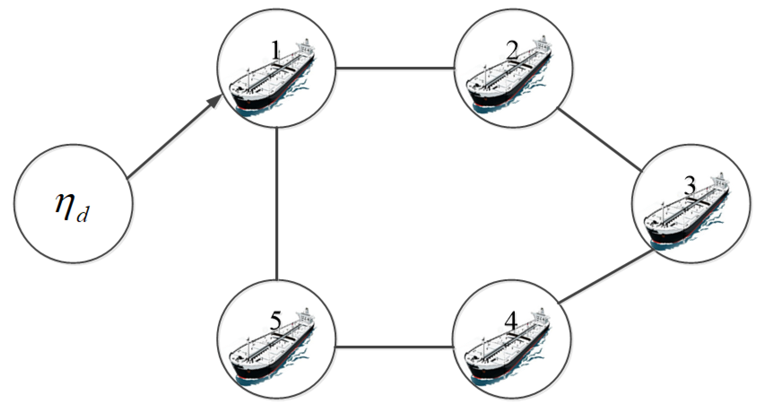
2.1. Basic Concepts of Graph Theory

Define an undirected connected weighted graph $\wp =\wp (\nu ,\ell )$, where $\nu =\left\{1,2,\cdots ,n\right\}$ represents the set of vessels, $\ell \subseteq \nu \times \nu$ is the set of edges, and ${\ell }_{ij}=(i,j)$ represents that node j can obtain the information of node i. $(j,i)\in \ell$ expresses that node i is a neighbor of node j and $N_i=\left\{j\in \nu \left|(j,i)\in \ell \right.\right\}$ represents the set of neighbors of node i. $A=\left[a_{ij}\right]\in {\Re }^{n\times n}$ is the weighted adjacency matrix. The Laplacian matrix $D=\left[d_{ij}\right]\in {\Re }^{n\times n}$ is defined as $D(i,j)=\left\{\begin{array}{cc}{\sum }_{j\in N_i}{a}_{ij},\hfill & i=j\hfill \\ 0,\hfill & i\ne j\hfill \end{array}\right.$. In the same way, $L=\left[l_{ij}\right]\in {\Re }^{n\times n}$ is defined as $l_{ij}=\left\{\begin{array}{cc}-a_{ij},\hfill & i=j\hfill \\ {\sum }_{j=1,j\ne i}^n{a}_{ij},\hfill & i\ne j\hfill \end{array}\right.$. $I_n$ represents the feature vectors of L. Let $B=\mathrm{diag}\left\{b_1,b_2,\cdots ,b_n\right\}$ be the adjacency matrix, where $\mathrm{diag}(·)$ denotes the diagonal matrix. $b_i>0$ means that the ith vessel is accessible to the leader and $b_i=0$ represents the other case [38].

2.2. System Modeling

The following mathematical model of multi-vessel motion [39] is presented based on the earth-fixed (O-NED) and body-fixed (B-XYZ) frames, as shown in Figure 1:

$$\left\{\begin{array}{c}{\dot{\eta }}_i=R\left({\psi }_i\right)v_i\hfill \\ M_i{\dot{v}}_i+C_i\left(v_i\right)v_i+D_i\left(v_i\right)v_i+g\left(v_i\right)={\tau }_i+{\tau }_{wi}\hfill \end{array}\right.i=1,2,\cdots ,n$$

(1)

where n is the number of vessels in the formation system and i represents the ith vessel. $M_i$ represents the system inertia matrix, which can be obtained in practical engineering applications; $C_i\left(v_i\right)$ and $D_i\left(v_i\right)$ represent the centripetal force matrix and damping coefficient matrix, respectively; $g\left(v_i\right)$ is the unmodeled dynamics; ${\eta }_i$ and $v_i$ denote the position and velocity vectors; ${\tau }_i$ is the control force vector; ${\tau }_{wi}$ is the time-varying environmental disturbance vector; and $R\left({\psi }_i\right)$ represents the conversion matrix between the two coordinate frames shown in Figure 1:

$$\begin{array}{c}\hfill R\left({\psi }_i\right)=\left[\begin{array}{ccc}cos\left({\psi }_i\right)& -sin\left({\psi }_i\right)& 0\\ sin\left({\psi }_i\right)& cos\left({\psi }_i\right)& 0\\ 0& 0& 1\end{array}\right]\end{array}$$

(2)

A new vector ${\mu }_i={\dot{\eta }}_i$ is defined for (1), which yields:

$$\left\{\begin{array}{c}{\mu }_i={\dot{\eta }}_i\hfill \\ {\dot{\mu }}_i=R_i{M_i}^{-1}{\tau }_i+W_i\hfill \end{array}\right.i=1,2,\cdots ,n$$

(3)

where $W_i=R_i{M_i}^{-1}({\tau }_{wi}-g_i\left(v_i\right))+S\left(r_i\right){\mu }_i-R_i{M_i}^{-1}(C\left(v_i\right)+D\left(v_i\right)){R_i}^T{\mu }_i$ represents the total system uncertainties, and $S\left(r_i\right)=\left[\begin{array}{ccc}0& -r_i& 0\\ r_i& 0& 0\\ 0& 0& 1\end{array}\right]$.

Assumption A1

([1]). The system uncertainties $W_i$ satisfy $∥{\dot{W}}_i∥\le \iota$ with a positive boundary ι.

Remark 1

([40]). Since the energies of vessels and the ocean environment are finite, the system uncertainties $W_i$ should be considered as bounded with a finite rate. There are low- and high-frequency external disturbances. The high-frequency disturbances do not contribute to the vessel’s movement. Based on the wave-filtering technique, high-frequency disturbances can be discarded when designing the formation controller. Thus, the disturbances can be considered low frequency, which means the disturbances are differentiable. Therefore, Assumption 1 is reasonable.

Assumption A2

([1]). The desired trajectory of the virtual leader ${\eta }_d\left(t\right)={\left[x_d,y_d,{\psi }_d\right]}^T$ is bounded and differentiable with bounded ${\dot{\eta }}_d$ and ${\ddot{\eta }}_d$.

2.3. Nonlinear Extended State Observer

A nonlinear ESO is given to estimate the system uncertainties and velocities of the vessels [20]:

$$\left\{\begin{array}{c}{z}_{i1}={\gamma }^2({\eta }_i-{\hat{\eta }}_i)\hfill \\ {\dot{\hat{\eta }}}_i={\hat{\mu }}_i+({\beta }_1/\gamma ){\phi }_{i1}(z_{i1},{\theta }_1)\hfill \\ {\dot{\hat{\mu }}}_i={\hat{W}}_i+{\beta }_2{\phi }_{i2}(z_{i1},{\theta }_2)+R_i{M_i}^{-1}{\tau }_i\hfill \\ {\dot{\hat{W}}}_i=\gamma {\beta }_3{\phi }_{i3}(z_{i3},{\theta }_3)\hfill \end{array}\right.$$

(4)

where ${\hat{\eta }}_i$ and ${\hat{\mu }}_i$ are the observed position and velocity vectors in the O-NED frame of the vessel; ${\hat{W}}_i$ are the observed system uncertainties; and ${\theta }_1\in (2/3,1)$, ${\theta }_2=2{\theta }_1-1$, ${\theta }_3=3{\theta }_1-2$; ${\beta }_1>0$, ${\beta }_2>0$ and ${\beta }_3>0$ represent the observer gains. The function ${\phi }_{ij}(·)$ is given by:

$${\varphi }_{ij}(z_{1i},{\theta }_j)=\left\{\begin{array}{c}{z}_{1i},\left|z_{1i}\right|\le 1\hfill \\ {\left|z_{1i}\right|}^{{\theta }_j}sign\left(z_{1i}\right),\left|z_{1i}\right|>1\hfill \end{array}\right.j=1,2,3$$

(5)

where $\left|·\right|$ is the absolute value of a scalar. Then, define two new vectors $z_{2i}=\gamma ({\mu }_i-{\hat{\mu }}_i)$, $z_{3i}=W_i-{\hat{W}}_i$. Therefore, the estimation error system can be given by:

$$\left\{\begin{array}{c}{\dot{z}}_{i1}=\gamma (z_{i2}-{\beta }_1{\phi }_{i1}(z_{i1},{\theta }_1))\hfill \\ {\dot{z}}_{i2}=\gamma (z_{i3}-{\beta }_2{\phi }_{i2}(z_{i1},{\theta }_2))\hfill \\ {\dot{z}}_{i3}=\gamma ({\hat{W}}_i/\gamma -{\beta }_3{\phi }_{i3}(z_{i1},{\theta }_3))\hfill \end{array}\right.$$

(6)

Theorem 1.

For System (3) with the proposed nonlinear ESO (4), under Assumptions 1 and 2 for any given initial ${\eta }_i$ and $v_i$, the observation errors ${\chi }_{i1}={\eta }_i-{\hat{\eta }}_i$, ${\chi }_{i2}={\mu }_i-{\hat{\mu }}_i$, ${\chi }_{i3}=W_i-{\hat{W}}_i$ are bounded:

$$\begin{array}{c}\hfill \left|{\chi }_{ij}\right|\le \frac{1}{{\gamma }^{n+1-j}\sqrt{{\lambda }_{min}\left(P_i\right)}}{\left(\frac{{\lambda }_{max}\left(P_i\right)(2\iota +2\gamma \epsilon ∥\beta ∥)}{c_{1i}}\right)}^{1/{\theta }_1}\end{array}$$

(7)

where $P_i$ is an arbitrary positive-definite symmetric matrix, $∥·∥$ is the Euclidean norm of a vector, and ${\lambda }_{min}(·)$ and ${\lambda }_{max}(·)$ denote the minimum and maximum eigenvalues of a matrix.

Proof of Theorem 1.

Define the new vectors as follows:

$$\begin{array}{c}\hfill Z_i={\left[{z_{1i}}^T,{z_{2i}}^T,{z_{3i}}^T\right]}^T\end{array}$$

(8)

$$\begin{array}{c}\hfill F\left(Z_i\right)=\left(\begin{array}{c}{z}_{i2}-{\beta }_1{\left|z_{i1}\right|}^{{\theta }_1}\mathrm{sign}\left(z_{i1}\right)\\ z_{i3}-{\beta }_2{\left|z_{i1}\right|}^{\theta 2}\mathrm{sign}\left(z_{i1}\right)\\ -{\beta }_3{\left|z_{i1}\right|}^{{\theta }_3}\mathrm{sign}\left(z_{i1}\right)\end{array}\right)\end{array}$$

(9)

$$\begin{array}{c}\hfill G\left(Z_i\right)=\left(\begin{array}{c}{z}_{i2}-{\beta }_1{\phi }_i(z_{i1},{\theta }_1)\\ z_{i3}-{\beta }_2{\phi }_i(z_{i1},{\theta }_2)\\ -{\beta }_3{\phi }_i(z_{i1},{\theta }_3)\end{array}\right)\end{array}$$

(10)

Based on (6), we obtain:

$$\begin{array}{c}\hfill \frac{\mathrm{d}{Z}_i}{\mathrm{d}t}=\gamma G\left(Z_i\right)+\left[\begin{array}{ccc}0& 0& {\dot{W}}_i\end{array}\right]\end{array}$$

(11)

Define the following Lyapunov function for (6):

$$\begin{array}{c}\hfill V_1\left(Z_i\right)={Z_i}^T{P}_i{Z}_i\end{array}$$

(12)

Based on the theory of homogeneity, (6) has the homogeneity ${\theta }_1-1$ under the weight $(1,{\theta }_1-1,2{\theta }_2-1)$. Similarly, $V_1\left(Z_i\right)$ and $L_F{V}_1\left(Z_i\right)$ have the homogeneities 2 and ${\theta }_1+1$, where $L_F{V}_1\left(Z_i\right)$ denotes the L-th-order derivative of $V_1\left(Z_i\right)$ along $F\left(Z_i\right)$. By using Lemma 4.2 in [41], we can obtain $L_F{V}_1\left(Z_i\right)\le -c_{i1}{V}_1{\left(Z_i\right)}^{\varsigma }$, $c_{i1}=-\underset{\left\{Z_i:V_1\left(Z_i\right)=1\right\}}{max}{L}_F{V}_1\left(Z_i\right)$, $\varsigma =(1+{\theta }_1)/2$. According to (5), if $\left|z_{1i}\right|>1$, $F\left(Z_i\right)=G\left(Z_i\right)$; otherwise, $∥G\left(Z_i\right)-F\left(Z_i\right)∥\le ∥\beta ∥\underset{\left|z_{1i}\right|<1}{max}\left|z_{1i}-{\left|z_{1i}\right|}^{{\theta }_j}\mathrm{sign}\left(z_{1i}\right)\right|$, where $\beta ={\left[\begin{array}{ccc}{\beta }_1& {\beta }_2& {\beta }_3\end{array}\right]}^T$.

The following formula can be easily obtained:

$$\begin{array}{c}\hfill \underset{{\theta }_j\to 1}{lim}\underset{\left|z_{1i}<1\right|}{max}\left|z_{i1}-{\left|z_{i1}\right|}^{{\theta }_j}\mathrm{sign}({\mathrm{z}}_{\mathrm{i}1})\right|=0\end{array}$$

(13)

Design a parameter as follows:

$$\begin{array}{c}\hfill \upsilon =min\left\{\frac{\gamma c_{1i}-2\iota {\lambda }_{max}\left(P_i\right)}{2\gamma ∥\beta ∥{\lambda }_{max}\left(P_i\right)},\frac{\gamma c_{i1}\underset{z_i}{min}(V_1{\left(Z_i\right)}^{\varsigma -1/2}-2\iota {\lambda }_{max}\left(P_i\right))}{2\gamma ∥\beta ∥{\lambda }_{max}\left(P_i\right)}\right\}\end{array}$$

(14)

Then we obtain $\underset{1\le i\le 3,\left|z_{i1}<1\right|}{max}\left|z_{i1}-{\left|z_{i1}\right|}^{{\theta }_j}\mathrm{sign}\left(z_{i1}\right)\right|<\upsilon$. Take the derivative of $V_1\left(Z_i\right)$:

$$\begin{array}{cc}\hfill {\dot{V}}_1\left(Z_i\right)& \le -\gamma c_{1i}{V}_1{\left(Z_i\right)}^{\varsigma }+2{\lambda }_{max}\left(P_i\right)\iota ∥Z_i∥+2\gamma \upsilon {\lambda }_{max}\left(P_i\right)∥\beta ∥∥Z_i∥\hfill \\ \hfill & \le -\gamma c_{1i}{V}_1{\left(Z_i\right)}^{\varsigma }+(2\iota +2\gamma \upsilon ∥\beta ∥){\lambda }_{max}\left(P_i\right)V_1{\left(Z_i\right)}^{1/2}\hfill \end{array}$$

(15)

For (15), further analysis is discussed in two cases:

Case 1.

$V_1\left(Z_i\right)\ge 1$

We have $\varsigma =(1+{\theta }_1)/2$ so (15) can be simplified to:

$$\begin{array}{c}\hfill {\dot{V}}_1\left(Z_i\right)\le -\left[\gamma c_{1i}-{\lambda }_{max}\left(P_i\right)\left(2\gamma \upsilon ∥\beta ∥\right)\right]V_1{\left(Z_i\right)}^{\varsigma }\end{array}$$

(16)

Choose the appropriate parameters for γ, ${\beta }_j$, and $P_i$:

$$\gamma >max\left\{2\iota {\lambda }_{max}\left(P_i\right)/(c_{1i}-2\upsilon {\lambda }_{max}\left(P_i\right)∥\beta ∥\right.$$

(17)

Then, we obtain ${\dot{V}}_1\left(Z_i\right)<0$.

Case 2.

$V_1\left(Z_i\right)<1$

Let:

$$0<\epsilon <1-(2\iota +2\gamma \upsilon ∥\beta ∥){\lambda }_{max}\left(P_i\right)/\left(\gamma c_{1i}\right)$$

(18)

We obtain:

$$\begin{array}{cc}\hfill {\dot{V}}_1\left(Z_i\right)\le & -\left[\gamma c_{1i}(1-\epsilon )V_1{\left(Z_i\right)}^{\varsigma }-(2\iota +2\gamma \upsilon ∥\beta ∥){\lambda }_{max}\left(P_i\right)V_1{\left(Z_i\right)}^{1/2}\right]\hfill \\ \hfill & -\gamma c_{1i}\epsilon V_1{\left(Z_i\right)}^{\varsigma }\hfill \\ \hfill \le & -\left[\gamma c_{1i}(1-\epsilon )V_1{\left(Z_i\right)}^{\varsigma -1/2}-(2\iota +2\gamma \upsilon ∥\beta ∥){\lambda }_{max}\left(P_i\right)\right]V_1{\left(Z_i\right)}^{1/2}\hfill \\ \hfill & -\gamma c_{1i}\epsilon V_1{\left(Z_i\right)}^{\varsigma }\hfill \end{array}$$

(19)

If $V_1\left(Z_i\right)>{\lambda }_{max}\left(P_i\right)(2\iota -2\gamma \upsilon ∥\beta ∥)/\left(c_{1i}\gamma (1-\epsilon )\right)$, the system is stable and we have:

$$\begin{array}{c}\hfill {\dot{V}}_1\left(Z_i\right)<{\left({\lambda }_{max}\left(P_i\right)(2\iota -2\gamma \upsilon ∥\beta ∥)/\left(c_{1i}\gamma (1-\epsilon )\right)\right)}^{2/(2\varsigma -1)}\end{array}$$

(20)

According to (20), we have:

$$\begin{array}{c}\hfill ∥Z_i∥<\frac{1}{\sqrt{{\lambda }_{max}\left(P_i\right)}}{\left(\frac{{\lambda }_{max}\left(P_i\right)(2\iota +2\gamma \upsilon ∥\beta ∥)}{c_{1i}\gamma (1-\epsilon )}\right)}^{1/{\theta }_1}\end{array}$$

(21)

Hence, the proof of Theorem 1 is completed. □

2.4. Prescribed Performance

The following performance specifications are imposed on the formation errors to improve the performance of the control system.

$$\begin{array}{c}\hfill -{\delta }_1\rho \left(t\right)<{\xi }_i\left(t\right)<{\delta }_2\rho \left(t\right),\forall t>0\end{array}$$

(22)

It should be noted that the conventional PPF is asymptotically convergent, which may result in infinite convergence times. Since finite-time stability can drive the system states to equilibrium in finite time, an FTPPF is designed to overcome the drawback of the conventional PPF. Firstly, a definition for the FTPPF is given as follows:

Definition 1

([33]). If the following properties are able to be satisfied for a continuous function $\rho \left(t\right)$:

$$\left\{\begin{array}{c}\rho \left(t\right)>0,\dot{\rho }\left(t\right)\le 0\hfill \\ \underset{t\to T_f}{lim}\rho \left(t\right)={\rho }_{T_f}>0\hfill \\ \rho \left(t\right)={\rho }_{T_f},t\ge T_f\hfill \end{array}\right.$$

(23)

where ${\rho }_{T_f}$ is an arbitrarily small constant and $T_f$ is the set time, then $\rho \left(t\right)$ can be called the FTPPF.

Subsequently, an FTPPF is designed according to (22) and Definition 1, which is expressed as:

$$\rho \left(t\right)=\left\{\begin{array}{cc}({\rho }_0-\frac{t}{T_f})e^{k(1-\frac{T_f}{T_f-t})}+{\rho }_{T_f},\hfill & t\in [0,T_f)\hfill \\ {\rho }_{T_f},\hfill & t\in [T_f,+\infty )\hfill \end{array}\right.$$

(24)

where ${\rho }_0$, ${\rho }_{T_f}$, and k are positive constants.

The curves of $\rho \left(t\right)$ under different $T_f$ are shown in Figure 2. As shown in the figure, tuning the design parameters $T_f$ can lead to different forms of the constraint boundary. $\rho \left(t\right)$ also conforms with Definition 1. The errors can meet the preset transient and steady-state performance with the proper selection of these parameters.

As can be seen, the designed FTPPF has two benefits: it can achieve the finite-time convergence of tracking errors in the prescribed stability areas, which is practical; and $T_f$ can be set by users in advance, which can be achieved more easily than the conventional PPF.

3. Design and Analysis

Firstly, a distributed formation error is designed in Section 3.1. Then, an error transformation is proposed for the formation error. Subsequently, the distributed formation controller is designed using dynamic surface control technology. The stability of the distributed formation system is proved in Section 3.2.

3.1. Controller Design

A distributed formation controller incorporating the proposed FTPPF and dynamic surface control method is designed for multi-vessel formation control under multiple constraints.

Based on the adjacent rule, the first formation error is defined as follows:

$$\begin{array}{c}\hfill {\xi }_{i1}={\sum }_{j\in N_i}{a}_{ij}({\eta }_i+R\left({\psi }_i\right)l_i-{\eta }_j-R\left({\psi }_j\right)l_j)+b_i({\eta }_i+R\left({\psi }_j\right)l_j-{\eta }_d)\end{array}$$

(25)

where ${\eta }_d$ is the desired position of the vessels.

Take the derivative of ${\xi }_{i1}$ as:

$$\begin{array}{c}\hfill {\dot{\xi }}_{i1}=d_{bi}{\hat{\mu }}_i+d_{bi}\dot{R}\left({\psi }_i\right)l_i-{\sum }_{j\in N_i}{a}_{ij}{\hat{\mu }}_j-{\sum }_{j\in N_i}{a}_{ij}\dot{R}\left({\psi }_j\right)l_j-b_i{\dot{\eta }}_d\end{array}$$

(26)

In (26), $d_{bi}=d_{ii}+b_i$, $d_{ii}$ is the element of the Laplacian matrix.

Based on (22), the following error transformation is constructed to facilitate the controller design:

$$\left\{\begin{array}{c}{\xi }_{i1}=\rho \left(t\right)T\left(s_i\right)\hfill \\ T\left(s_i\right)=\frac{{\delta }_2{e}^{s_i}-{\delta }_1{e}^{s_i}}{e^{s_i}+e^{-s_i}}\hfill \end{array}\right.$$

(27)

where $T\left(s_i\right)$ is strictly monotonic increasing and $s_i=\frac{1}{2}ln\left(\frac{{\xi }_{i1}+{\delta }_1\rho \left(t\right)}{{\delta }_2\rho \left(t\right)-{\xi }_{i1}}\right)$.

Then, choose the following error transformation:

$$\begin{array}{c}\hfill o_i=s_i-\frac{1}{2}ln({\delta }_1/{\delta }_2)\end{array}$$

(28)

Take the derivative of $o_i$ as

$$\begin{array}{c}\hfill {\dot{o}}_i={\sigma }_i({\dot{\xi }}_{i1}-{\xi }_{i1}\dot{\rho }/\rho )\end{array}$$

(29)

where ${\sigma }_i=(1/2({\xi }_{i1}+{\delta }_1\rho )-1/2({\xi }_{i1}-{\delta }_2\rho ))>0$.

The following virtual control law based on the backstepping method is designed:

$$\begin{array}{c}\hfill \begin{array}{c}{\alpha }_i=\frac{1}{{\sigma }_i{d}_{bi}}\left[-{\varpi }_1{o}_i-{\sigma }_i(d_{bi}\dot{R}\left({\psi }_i\right)l_i-\right.\hfill \\ \left.{\sum }_{j\in N_i}{a}_{ij}{\hat{\mu }}_j-{\sum }_{j\in N_i}{a}_{ij}\dot{R}\left({\psi }_i\right)l_j-b_i{\dot{\eta }}_d)+{\sigma }_i{\xi }_{i1}\dot{\rho }/\rho \right]\hfill \end{array}\end{array}$$

(30)

where ${\varpi }_1$ is the parameter to be designed.

To avoid differential expansion, dynamic surface control technology is introduced:

$$\left\{\begin{array}{c}{T}_d{\dot{\alpha }}_{di}+{\alpha }_{di}={\alpha }_i\hfill \\ {\alpha }_{di}\left(0\right)={\alpha }_i\left(0\right)\hfill \end{array}\right.$$

(31)

where the time constant $T_d$ is positive and ${\alpha }_{di}$ is the guidance law for the velocities.

Define a new error ${\alpha }_{{\xi }_i}={\alpha }_{di}-{\alpha }_i$, where we have:

$$\begin{array}{c}\hfill {\dot{\alpha }}_{{\xi }_i}=-{\alpha }_{{\xi }_i}/T_d+{\Delta }_i({\xi }_{i1},{\xi }_{i2},{\alpha }_{{\xi }_i},{\alpha }_{{\xi }_j},S_i,{\dot{S}}_i,{\dot{S}}_j,{\dot{S}}_j,{\ddot{\eta }}_d)\end{array}$$

(32)

where ${\Delta }_i(·)=\frac{1}{d_{bi}}({\varpi }_1{\dot{\xi }}_{i1}+d_{bi}\dot{R}\left({\psi }_i\right)S_i{l}_i+d_{bi}R\left({\psi }_i\right){\dot{S}}_i{l}_i-{\sum }_{j\in N_i}{a}_{ij}{\ddot{\eta }}_j-{\sum }_{j\in N_i}{a}_{ij}\dot{R}\left({\psi }_j\right)S_j{l}_j-{\sum }_{j\in N_i}{a}_{ij}R\left({\psi }_j\right){\dot{S}}_j{l}_j-b_i{\ddot{\eta }}_d)$.

Consider that the initial states of the system are bounded and we have $∥{\Delta }_i(·)∥\le {\overline{\Delta }}_i$ under Assumption 2.

The velocity tracking error is defined as follows:

$$\begin{array}{c}\hfill {\xi }_{i2}={\hat{\mu }}_i-{\alpha }_{di}\end{array}$$

(33)

Based on (31) and (33), we take the derivative of ${\xi }_{i2}$ as:

$$\begin{array}{c}\hfill {\dot{\xi }}_{i2}={\hat{f}}_i+{\beta }_2{\phi }_i(z_{i1},{\theta }_2)=R{M_i}^{-1}{\tau }_i-{\dot{\alpha }}_{di}\end{array}$$

(34)

where $\hat{f}$ is the estimate of the system uncertainties from the nonlinear ESO.

Therefore, design the formation control law as follows:

$$\begin{array}{c}\hfill {\tau }_i=M_i{R}^T\left({\psi }_i\right)\left[-{\varpi }_2{\xi }_{i2}-{\hat{f}}_i-{\beta }_2{\phi }_i(z_{i1},{\theta }_2)+{\dot{\alpha }}_{di}\right]\end{array}$$

(35)

where ${\varpi }_2$ is the designed parameter.

Let $\mathrm{\Theta }=(D+B)\otimes I_3$, $\mathrm{\Gamma }=(L+B)\otimes I_3$, $E_1={\left[{{\xi }_{11}}^T,{{\xi }_{21}}^T,\cdots ,{{\xi }_{n1}}^T\right]}^T$, $O=[{o_1}^T,{o_2}^T,\cdots ,$${o_n}^T{]}^T$, $\mathrm{\Lambda }=\mathrm{dia}{\mathrm{g}}_{i\in \left\{1,2,\cdots ,n\right\}}\left({\sigma }_i\right)$, $\Delta ={\left[{{\Delta }_1}^T,{{\Delta }_2}^T,\cdots ,{{\Delta }_n}^T\right]}^T$, $E_2={\left[{{\xi }_{12}}^T,{{\xi }_{22}}^T,\cdots ,{{\xi }_{n2}}^T\right]}^T$, $z_2={\left[{z_{12}}^T,{z_{22}}^T,\cdots ,{z_{n2}}^T\right]}^T$, and ${\alpha }_{\xi }={\left[{{\alpha }_{{\xi }_1}}^T,{{\alpha }_{{\xi }_2}}^T,\cdots ,{{\alpha }_{{\xi }_n}}^T\right]}^T$ and we obtain the system of the formation error as follows:

$$\left\{\begin{array}{c}\dot{O}=\mathrm{\Lambda }{\dot{E}}_1-\mathrm{\Lambda }\dot{\rho }{E}_1/\dot{\rho }\hfill \\ {\dot{E}}_2=-{\varpi }_2{E}_2\hfill \end{array}\right.$$

(36)

Define the following Lyapunov function:

$$\begin{array}{c}\hfill V_2=\frac{1}{2}(O^{T}O+{E_2}^T{E}_2+{{\alpha }_{\xi }}^T{\alpha }_{\xi })\end{array}$$

(37)

Take the derivative of $V_2$ as:

$$\begin{array}{cc}\hfill {\dot{V}}_2& =O^T\mathrm{\Lambda }({\dot{E}}_1-\dot{\rho }{E}_1/\rho )-{\varpi }_2{E_2}^T{E}_2-{{\alpha }_{\xi }}^T(\Delta -{\alpha }_{\xi }/T_d)\hfill \\ \hfill \le & -\mathrm{\Lambda }{\varpi }_1{O}^T{E}_1+{\lambda }_{max}\left(\mathrm{\Theta }\right)\mathrm{\Lambda }{O}^T{E}_2+{\lambda }_{max}\left(\mathrm{\Theta }\right)\mathrm{\Lambda }{O}^T{\alpha }_{\xi }\hfill \\ \hfill & -{\varpi }_2{E_2}^T{E}_2+{\lambda }_{max}\left(\mathrm{\Gamma }\right)\mathrm{\Lambda }\left|O^T{z}_2\right|/\gamma -{{\alpha }_{\xi }}^T{\alpha }_{\xi }/T_d+\left|{{\alpha }_{\xi }}^T\Delta \right|\hfill \\ \hfill & -\rho \mathrm{\Lambda }{O}^T{E}_1\hfill \end{array}$$

(38)

Based on Young’s inequality [42], (38) is rewritten as:

$$\begin{array}{cc}\hfill {\dot{V}}_2& \le (\frac{{\lambda }_{max}\left(\mathrm{\Gamma }\right)}{2\gamma }+{\lambda }_{max}\left(\mathrm{\Theta }\right)-\frac{{\varpi }_1}{2}-\frac{\dot{\rho }}{2\rho })\mathrm{\Lambda }{∥O∥}^2+\frac{{\lambda }_{max}\left(\mathrm{\Gamma }\right)\mathrm{\Lambda }}{2\gamma }{∥z_2∥}^2\hfill \\ \hfill & +(\frac{{\lambda }_{max}\left(\mathrm{\Theta }\right)\mathrm{\Lambda }}{2}-\frac{1}{T_d}+\frac{{∥\Delta (·)∥}^2}{2}){∥{\alpha }_{\xi }∥}^2+(\frac{{\lambda }_{max}\left(\mathrm{\Theta }\right)\mathrm{\Lambda }}{2}-{\varpi }_2){∥E_2∥}^2\hfill \\ \hfill & -(\frac{{\varpi }_1\mathrm{\Lambda }}{2}+\frac{\dot{\rho }\mathrm{\Lambda }}{2\rho }){∥E_1∥}^2+\frac{1}{2}\hfill \end{array}$$

(39)

Design the parameter ${\omega }_j>0,j=1,2,3$ as follows:

$$\left\{\begin{array}{c}{\omega }_1\le -\mathrm{\Lambda }(\frac{{\lambda }_{max}\left(\mathrm{\Gamma }\right)}{2\gamma }+{\lambda }_{max}\left(\mathrm{\Theta }\right)-\frac{{\varpi }_1}{2}-\frac{\dot{\rho }}{2\rho })\hfill \\ {\omega }_2\le -\frac{{\lambda }_{max}\left(\mathrm{\Theta }\right)\mathrm{\Lambda }}{2}+{\varpi }_2\hfill \\ {\omega }_3\le -\frac{{\lambda }_{max}\left(\mathrm{\Theta }\right)\mathrm{\Lambda }}{2}+\frac{1}{T_d}-\frac{{∥\Delta (·)∥}^2}{2}\hfill \end{array}\right.$$

(40)

Then, (39) can be simplified to:

$$\begin{array}{cc}\hfill {\dot{V}}_2& \le \frac{{\lambda }_{max}\left(\mathrm{\Gamma }\right)\mathrm{\Lambda }}{2\gamma }{∥z_2∥}^2-(\frac{{\varpi }_1\mathrm{\Lambda }}{2}+\frac{\dot{\rho }\mathrm{\Lambda }}{2\rho }){∥E_1∥}^2\hfill \\ \hfill & -(1-\frac{{∥\Delta (·)∥}^2}{{\overline{\Delta }}^2})\frac{{\overline{\Delta }}^2}{2}{∥{\alpha }_{\xi }∥}^2+2\omega V_2+\frac{1}{2}\hfill \\ \hfill & \le 2\omega V_2+\frac{1}{2}+\frac{{\lambda }_{max}\left(\mathrm{\Gamma }\right)\mathrm{\Lambda }}{2\gamma }{∥z_2∥}^2\hfill \end{array}$$

(41)

where $\omega =min\left\{{\omega }_1,{\omega }_2,{\omega }_3\right\}$.

3.2. Stability Analysis

Theorem 2.

Consider a multiple-vessel system (3) with unmeasurable velocities and system uncertainties, combined with the nonlinear ESO and proposed FTPPF. Under Assumption 2, for any given constant $V_M>0$ based on the estimation of the nonlinear ESO and (35), if the initial states of the system have ${\sum }_{i=1}^n{V}_1\left(Z_i\right)+V_2\le V_M$, then all signals of System (3) are bounded and ${\xi }_{i1}$ can converge to a small-enough FTPPF-based set within the set time $T_f$, which means that the formation errors of multiple vessels can approach zero.

Proof 

(Proof of Theorem 2). Construct the following Lyapunov function:

$$\begin{array}{c}\hfill V_3={\sum }_{i=1}^n{V}_1\left(Z_i\right)+V_2\end{array}$$

(42)

Take the derivative of $V_3$ based on (15) and (41) and we have:

$$\begin{array}{cc}\hfill {\dot{V}}_3\le & -{\sum }_{i=1}^n\left[\gamma c_{1i}(1-\epsilon )V_1{\left(Z_i\right)}^{\varsigma -1/2}\right.\hfill \\ \hfill & \left.-(2\iota +2\gamma \upsilon ∥\beta ∥){\lambda }_{max}\left(P_i\right)\right]V_1{\left(Z_i\right)}^{1/2}\hfill \\ \hfill & -{\sum }_{i=1}^n\gamma c_{1i}\epsilon V_1{\left(Z_i\right)}^{\varsigma }+\frac{1}{2}-2\omega V\hfill \\ \hfill & +{\sum }_{i=1}^n\left({\lambda }_{max}\left(\mathrm{\Gamma }\right)/\left(2\gamma {\lambda }_{min}\left(P_i\right)\right)\right)V_1\left(Z_i\right)\hfill \\ \hfill \le & -{\sum }_{i=1}^n{V}_1{\left(Z_i\right)}^{\varsigma }\left[\gamma c_{1i}\epsilon -(2\omega +{\lambda }_{max}\left(\mathrm{\Gamma }\right)/\left(2\gamma {\lambda }_{min}\left(P_i\right)\right))V_1^{1-\varsigma }\right]\hfill \\ \hfill & -{\sum }_{i=1}^n\left[\gamma c_{1i}(1-\epsilon )V_1{\left(Z_i\right)}^{\varsigma -1/2}\right..-(2{\iota }_i+2\gamma \upsilon ∥\beta ∥){\lambda }_{max}\left(P_i\right)]V_1{\left(Z_i\right)}^{1/2}\hfill \\ \hfill & -2\omega {\sum }_{i=1}^n{V}_1\left(Z_i\right)+\frac{1}{2}-2\omega V_2\hfill \end{array}$$

(43)

By selecting the appropriate parameters, $\gamma c_{1i}\epsilon -(2\omega +{\lambda }_{max}\left(\mathrm{\Gamma }\right)/\left(2\gamma {\lambda }_{min}\left(P_i\right)\right))V_1^{1-\varsigma }>0$ can be satisfied. In addition, according to (18), we have $\gamma c_{1i}(1-\epsilon )V_1{\left(Z_i\right)}^{\varsigma -1/2}-(2{\iota }_i+2\gamma \upsilon ∥\beta ∥){\lambda }_{max}\left(P_i\right)>0$. So, (43) can be rewritten as:

$$\begin{array}{c}\hfill {\dot{V}}_3\le -2\omega V_3+\frac{1}{2}\end{array}$$

(44)

Then, we obtain:

$$\begin{array}{c}\hfill V_3\le \frac{1}{4\omega }+(V_3\left(0\right)-\frac{1}{4\omega }){\mathrm{e}}^{-2\omega t}\end{array}$$

(45)

Based on (45), we have $V_3\le \frac{1}{4\omega }$. So, $\underset{t\to \infty }{lim}∥O∥\le \sqrt{\frac{1}{2\omega }}$, $\underset{t\to \infty }{lim}∥E_2∥\le \sqrt{\frac{1}{2\omega }}$, $\underset{t\to \infty }{lim}∥{\alpha }_{\xi }∥\le \sqrt{\frac{1}{2\omega }}$. Therefore, the errors O, $E_2$, and ${\alpha }_{\xi }$ are bounded with the appropriate parameters. Given (25) and (30)–(32), ${\eta }_i$, ${\alpha }_i$, ${\alpha }_{di}$, ${\alpha }_{{\xi }_i}$, and ${\xi }_{i2}$ are bounded. Since O is bounded, it is further concluded from (22) and (28) that ${\xi }_{i1}$ will converge to a small-enough FTPPF-based set $\mathrm{\Xi }=\left\{{\xi }_{i1}\left|-{\delta }_1\rho \left(t\right)<{\xi }_{i1}<{\delta }_2\rho \left(t\right)\right.\right\}$ within the set time $T_f$, which means the formation errors of multiple vessels can approach zero.

Hence, the proof of Theorem 2 is completed. □

4. Simulation Results and Comparative Analysis

To show the performance of the designed control method, simulations are conducted using a computer with Windows 11 and MATLAB 2022a. In the simulations, five vessels and one virtual leader are considered. The sizes of the five vessels are the same (the length is 44.79 m and the width is 6.2 m). The unmodeled dynamics and related main particulars of the vessels are given as follows:

$$\begin{array}{c}\hfill g_i={10}^3\times \left[\begin{array}{c}0.3u_i{v}_i^2+0.4v_i^2{r}_i\\ 0.1u_i{v}_i\\ 0.2u_i{r}_i^2+0.3u_i{r}_i{v}_i^3\end{array}\right]\end{array}$$

(46)

$$\begin{array}{c}\hfill M={10}^7\times \left[\begin{array}{ccc}0.0484& 0& 0\\ 0& 0.0901& 0.2192\\ 0& 0.2192& 5.3025\end{array}\right]\end{array}$$

(47)

$$\begin{array}{c}\hfill D={10}^5\times \left[\begin{array}{ccc}0.423+0.0142\left|u\right|& 0& 0\\ 0& 0.185+0.0385\left|v\right|+0.1275\left|r\right|& -1.089+1.276\left|v\right|+125.96\left|r\right|\\ 0& 2.295-0.3\left|v\right|+3.882\left|r\right|& 65.838+3.882\left|v\right|+6046.2\left|r\right|\end{array}\right]\end{array}$$

(48)

$$\begin{array}{c}\hfill C={10}^7\times \left[\begin{array}{ccc}0& 0& -0.0901v-0.2192r\\ 0& 0& 0.0484u\\ 0.0901v+0.2192r& -0.0484u& 0\end{array}\right]\end{array}$$

(49)

The environmental disturbances are set as in (50), with the first-order Markov process $\dot{\hslash }=-T^{-1}\hslash +A\overline{w}$ ([43,44]), where $\hslash \in {\Re }^3$ represents the bias forces and moment, $T\in {\Re }^{3\times 3}$ represents the time constant matrix, $\overline{w}\in {\Re }^3$ is the zero-mean Gaussian white noise, and $A\in {\Re }^{3\times 3}$ is used to scale the amplitude of $\overline{w}$.

$$\begin{array}{c}\hfill {\tau }_{wi}=R^T\left({\psi }_i\right)\hslash \end{array}$$

(50)

Choose $\hslash \left(0\right)={[2\times {10}^{4}N,1\times {10}^{6}N,2\times {10}^{7}Nm]}^T$, $T=diag({10}^3,{10}^3,{10}^3)$, and A = diag(100,100,100). The initial states are given as ${\eta }_1=-{\left[14,114,5^{\circ }\right]}^{\mathrm{T}}$, ${\eta }_2=-{\left[20,65,{25}^{\circ }\right]}^{\mathrm{T}}$, ${\eta }_3={\left[-28,-5,-{15}^{\circ }\right]}^T$, ${\eta }_4={\left[-30,66,-{10}^{\circ }\right]}^{\mathrm{T}}$, ${\eta }_5={\left[-5,117,-{20}^{\circ }\right]}^{\mathrm{T}}$, $u_i\left(0\right)=v_i\left(0\right)=0\left(\mathrm{m}/\mathrm{s}\right)$, and $r_i\left(0\right)=0\left(\mathrm{rad}/\mathrm{s}\right)$. The structure vectors in formation are $l_1={\left[0,100,0\right]}^{\mathrm{T}}$, $l_2={\left[0,50,0\right]}^{\mathrm{T}}$, $l_3={\left[0,0,0\right]}^{\mathrm{T}}$, $l_4={\left[0,-50,0\right]}^{\mathrm{T}}$, and $l_5={\left[0,-100,0\right]}^{\mathrm{T}}$. Through trial and error, the observer gains are set as ${\beta }_1=5$, ${\beta }_2=0.5$, and ${\beta }_3=0.1$ according to the estimation effect of the ESO. The control gains are designed as $T_f=150$ s, ${\rho }_{T_f}=3$, ${\rho }_0=100$, ${\theta }_1=0.7$, ${\theta }_2=0.4$, ${\theta }_3=0.1$, $\gamma =10$, $T_d=0.05$, ${\varpi }_1=0.5$, ${\varpi }_2=1$, ${\delta }_1=0.8$, ${\delta }_2=1$, and $k=2$. The expected trajectory is designed as:

$$\left\{\begin{array}{c}x\left(t\right)=2t\left(\mathrm{m}\right)\hfill \\ y\left(t\right)=0\left(\mathrm{m}\right)\hfill \end{array}\right.$$

(51)

The communication topology of multiple vessels is shown in Figure 3. It can be seen in Figure 3 that the communication topology of multiple vessels is undirected connected and only the first vessel can obtain the information of the expected trajectory. Due to confidentiality requirements, more details about the vessels cannot be provided. Nevertheless, it can be revealed that the communication devices on vessels can meet the requirements of two-way communication. Therefore, the undirected connected configuration is selected in this paper.

Moreover, the following conventional PPF and error transformation are constructed to show the superiority of our proposed FTPPF-based method:

$$\left\{\begin{array}{c}\underline{\rho }\left(t\right)=({\underline{\rho }}_0-{\underline{\rho }}_{\infty })e^{-t}+{\underline{\rho }}_{\infty }\hfill \\ \overline{\rho }\left(t\right)=({\overline{\rho }}_0-{\overline{\rho }}_{\infty })e^{-t}+{\overline{\rho }}_{\infty }\hfill \end{array}\right.$$

(52)

$$\left\{\begin{array}{c}{\xi }_{i1}=\underline{\rho }\left(t\right)T\left(o_i\right)\hfill \\ T\left(o_i\right)=(e^{o_i}-e^{-o_i})/(e^{o_i}-{\vartheta }^{-1}\left(t\right)e^{-o_i})\hfill \\ \vartheta \left(t\right)=\underline{\rho }\left(t\right)/\overline{\rho }\left(t\right)\hfill \end{array}\right.$$

(53)

$$o_i=\frac{1}{2}ln(1+\frac{{\xi }_{i1}}{\underline{\rho }\left(t\right)})-\frac{1}{2}ln(1-\frac{{\xi }_{i1}}{\overline{\rho }\left(t\right)})$$

(54)

In order to ensure comparability, the parameters of the conventional PPF and error transformation are consistent with those of the proposed FTPPF.

Then, to intuitively show the performance of the nonlinear ESO and proposed FTPPF-based formation controller, the simulation results for the estimation errors, trajectories of the vessels, formation errors, and control forces are provided below.

Figure 4 shows that the estimation errors of the nonlinear ESO can get close to zero after a period of time. This indicates that the observed values can approach the true velocities and system uncertainties, which can satisfy the design requirements of the subsequent formation controller. The trajectories of the vessels are shown in Figure 5. It can be seen in Figure 3 that only the first vessel can obtain the information of the expected trajectory, but all vessels can follow the desired trajectories with an expected formation. After maintaining a stable formation, it can be seen in the zoomed-in regions that all the deviations between the actual and the expected trajectories are less than 0.2 m, which meets the requirements of tracking accuracy.

Figure 6a–c show the formation errors under the proposed FTPPF-based controller, conventional PPF-based controller, and controller without PPF, respectively. It can be seen in Figure 6a–c that all the formation errors can finally converge to near zero under the three different control methods. In addition, it can be seen in Figure 6a that the convergence time under the proposed FTPPF-based controller is within the preset time $T_f$ = 150 s. Furthermore, in the zoomed-in areas in Figure 6a–c, we can see that the convergence time under the proposed FTPPF-based controller is approximately 100 s, which is smaller than the convergence times under the other two controllers (almost 110 s and 150 s). Moreover, compared with the zoomed-in areas in Figure 6b,c, the fluctuations of the formation errors are significantly reduced due to the smaller preset constraint bounds of our proposed FTPPF-based controller. Therefore, the superiority of our proposed FTPPF-based method is verified in Figure 6a–c. Figure 7 shows the surge, sway forces, and yaw moments for the vessels. As shown in the zoomed-in area in Figure 7, the control forces and moments are large at the beginning due to the initial large formation errors, as shown in Figure 6a, but maintain relatively small values after maintaining a stable formation.

Therefore, the proposed FTPPF-based formation controller can maintain multiple vessels in an expected formation with high tracking accuracy. In addition, our proposed FTPPF-based controller has a faster convergence speed and smaller fluctuations than a conventional PPF-based controller and a controller without PPF.

5. Conclusions

This paper presents a nonlinear ESO-based distributed formation control scheme with an FTPPF for multiple vessels, subject to unmeasurable velocities and system uncertainties. Initially, a nonlinear ESO is constructed to estimate the unmeasurable velocities and system uncertainties. Subsequently, a novel FTPPF is designed to improve the system transient performance, where the upper bound of the convergence time and constraint bounds can be flexibly preset without depending on the initial states and designed parameters. Then, a robust formation control scheme is presented based on the designed ESO and FTPPF. The boundedness can be guaranteed for all signals of the closed-loop system and the formation errors can approach zero within the preset time. Finally, simulations and comparisons show that our proposed FTPPF-based controller can maintain multiple vessels in an expected formation with high tracking accuracy, a faster convergence speed, and smaller fluctuations. However, collision avoidance is not considered in our proposed method, whose application would be limited in practice. Hence, collision avoidance will be the focus of future research in the design of a distributed formation controller.

References

1. Fu, M.; Yu, L. Finite-time extended state observer-based distributed formation control for marine surface vehicles with input saturation and disturbances. Ocean Eng. 2018, 159, 219–227. [Google Scholar] [CrossRef]
2. Zhang, L.; Jiao, J. Multi-surface ship formation control based on finite time observer. In Proceedings of the 2020 7th International Conference on Information, Cybernetics, and Computational Social Systems (ICCSS), Guangzhou, China, 13–15 November 2020; pp. 429–434. [Google Scholar]
3. Li, L.; Tuo, Y.; Li, T.; Tong, M.; Wang, S. Time-varying formation control of multiple unmanned surface vessels with heterogeneous hydrodynamics subject to actuator attacks. Appl. Math. Comput. 2022, 422, 126987. [Google Scholar] [CrossRef]
4. Liu, L.; Wang, D.; Peng, Z. ESO-Based Line-of-Sight Guidance Law for Path Following of Underactuated Marine Surface Vehicles With Exact Sideslip Compensation. IEEE J. Ocean. Eng. 2017, 42, 477–487. [Google Scholar] [CrossRef]
5. Kada, B.; Khalid, M.; Shaikh, M.S. Distributed cooperative control of autonomous multi-agent UAV systems using smooth control. J. Syst. Eng. Electron. 2020, 31, 1297–1307. [Google Scholar] [CrossRef]
6. Bae, Y.B.; Lim, Y.H.; Ahn, H.S. Distributed Robust Adaptive Gradient Controller in Distance-Based Formation Control With Exogenous Disturbance. IEEE Trans. Automat. Contr. 2021, 66, 2868–2874. [Google Scholar] [CrossRef]
7. Wang, R.; Dong, X.; Li, Q.; Ren, Z. Distributed Time-Varying Output Formation Control for General Linear Multiagent Systems With Directed Topology. IEEE Trans. Control Netw. 2019, 6, 609–620. [Google Scholar] [CrossRef]
8. Fossen, T.I. Marine Control Systems: Guidance, Navigation, and Control of Ships, Rigs and Underwater Vehicles; Marine Cybernetics: Trondheim, Norway, 2002. [Google Scholar]
9. Peng, Z.; Wang, J.; Wang, D. Distributed Maneuvering of Autonomous Surface Vehicles Based on Neurodynamic Optimization and Fuzzy Approximation. IEEE Trans. Contr. Syst. T. 2018, 26, 1083–1090. [Google Scholar] [CrossRef]
10. Liu, L.; Wang, D.; Peng, Z.; Chen, C.L.P.; Li, T. Bounded Neural Network Control for Target Tracking of Underactuated Autonomous Surface Vehicles in the Presence of Uncertain Target Dynamics. IEEE Trans. Neur. Net. Lear. 2019, 30, 1241–1249. [Google Scholar] [CrossRef]
11. Liu, L.; Wang, D.; Peng, Z.; Li, T. Modular Adaptive Control for LOS-Based Cooperative Path Maneuvering of Multiple Underactuated Autonomous Surface Vehicles. IEEE Trans. Syst. Man Cybern. Syst. 2017, 47, 1613–1624. [Google Scholar] [CrossRef]
12. He, S.; Dai, S.L.; Zhao, Z.; Zou, T. Uncertainty and disturbance estimator-based distributed synchronization control for multiple marine surface vehicles with prescribed performance. Ocean Eng. 2022, 261, 111867. [Google Scholar] [CrossRef]
13. Peng, Z.; Wang, J.; Wang, J. Constrained Control of Autonomous Underwater Vehicles Based on Command Optimization and Disturbance Estimation. IEEE Trans. Ind. Electron. 2019, 66, 3627–3635. [Google Scholar] [CrossRef]
14. Tuo, Y.; Wang, Y.; Wang, S. Reliability-Based Robust Online Constructive Fuzzy Positioning Control of a Turret-Moored Floating Production Storage and Offloading Vessel. IEEE Access 2018, 6, 36019–36030. [Google Scholar] [CrossRef]
15. Yu, C.; Xiang, X.; Wilson, P.A.; Zhang, Q. Guidance-Error-Based Robust Fuzzy Adaptive Control for Bottom Following of a Flight-Style AUV With Saturated Actuator Dynamics. IEEE Trans. Cybern. 2020, 50, 1887–1899. [Google Scholar] [CrossRef] [PubMed]
16. Wang, H.; Wang, D.; Peng, Z. Adaptive dynamic surface control for cooperative path following of marine surface vehicles with input saturation. Nonlinear Dynam. 2014, 77, 107–117. [Google Scholar]
17. Zheng, Z.; Sun, L. Path following control for marine surface vessel with uncertainties and input saturation. Neurocomputing 2016, 177, 158–167. [Google Scholar] [CrossRef]
18. Hao, W.; Dan, W.; Peng, Z. Neural network based adaptive dynamic surface control for cooperative path following of marine surface vehicles via state and output feedback. Neurocomputing 2014, 133, 170–178. [Google Scholar]
19. Peng, Z.; Dan, W.; Wang, J. Cooperative Dynamic Positioning of Multiple Marine Offshore Vessels: A Modular Design. IEEE/ASME Trans. Mech. 2016, 21, 1210–1221. [Google Scholar] [CrossRef]
20. Tuo, Y.; Wang, S.; Guo, C. Finite-time extended state observer-based area keeping and heading control for turret-moored vessels with uncertainties and unavailable velocities. Int. J. Nav. Arch. Ocean. 2022, 14, 100422. [Google Scholar] [CrossRef]
21. Peng, Z.; Wang, J.; Wang, D. Distributed Containment Maneuvering of Multiple Marine Vessels via Neurodynamics-Based Output Feedback. IEEE Trans. Ind. Electron. 2017, 64, 3831–3839. [Google Scholar] [CrossRef]
22. Bechlioulis, C.P.; Rovithakis, G.A. Robust Adaptive Control of Feedback Linearizable MIMO Nonlinear Systems With Prescribed Performance. IEEE Trans. Automat. Contr. 2008, 53, 2090–2099. [Google Scholar] [CrossRef]
23. Fan, A.; Li, J. Adaptive learning control synchronization for unknown time-varying complex dynamical networks with prescribed performance. Soft Comput. 2021, 25, 5093–5103. [Google Scholar] [CrossRef]
24. Zhu, L.; Li, T. Observer-Based Autopilot Heading Finite-Time Control Design for Intelligent Ship with Prescribed Performance. J. Mar. Sci. Eng. 2021, 9, 828. [Google Scholar] [CrossRef]
25. Wang, X.; Wang, Q.; Sun, C. Prescribed Performance Fault-Tolerant Control for Uncertain Nonlinear MIMO System Using Actor–Critic Learning Structure. IEEE Trans. Neur. Net. Lear. 2022, 33, 4479–4490. [Google Scholar] [CrossRef] [PubMed]
26. Chen, F.; Dimarogonas, D.V. Leader–Follower Formation Control With Prescribed Performance Guarantees. IEEE Trans. Control Netw. 2021, 8, 450–461. [Google Scholar] [CrossRef]
27. Zhang, G.; Cheng, D. Observer-based neuro-adaptive prescribed performance control of nonstrict feedback systems and its application. Optik 2019, 181, 264–277. [Google Scholar] [CrossRef]
28. Hu, Q.; Shao, X.; Guo, L. Adaptive Fault-Tolerant Attitude Tracking Control of Spacecraft With Prescribed Performance. IEEE/ASME Trans. Mech. 2018, 23, 331–341. [Google Scholar] [CrossRef]
29. Dai, S.L.; Wang, M.; Wang, C. Neural Learning Control of Marine Surface Vessels With Guaranteed Transient Tracking Performance. IEEE Trans. Ind. Electron. 2016, 63, 1717–1727. [Google Scholar] [CrossRef]
30. Zuo, Z.; Song, J.; Tian, B.; Basin, M. Robust Fixed-Time Stabilization Control of Generic Linear Systems With Mismatched Disturbances. IEEE Trans. Syst. Man Cybern. Syst. 2022, 52, 759–768. [Google Scholar] [CrossRef]
31. Azahar, M.I.P.; Irawan, A.; Ramli, M.S. Finite-Time Prescribed Performance Control for Dynamic Positioning of Pneumatic Servo System. In Proceedings of the 2020 IEEE 8th Conference on Systems, Process and Control (ICSPC), Virtual, 12th December 2020; pp. 1–6. [Google Scholar]
32. Sui, S.; Chen, C.L.P.; Tong, S. Finite-Time Adaptive Fuzzy Prescribed Performance Control for High-Order Stochastic Nonlinear Systems. IEEE Trans. Fuzzy Syst. 2022, 30, 2227–2240. [Google Scholar] [CrossRef]
33. Sun, K.; Guo, R.; Qiu, J. Fuzzy Adaptive Switching Control for Stochastic Systems With Finite-Time Prescribed Performance. IEEE Trans. Cybern. 2022, 52, 9922–9930. [Google Scholar] [CrossRef]
34. Dong, H.; Yang, X. Finite-Time Prescribed Performance Control for Space Circumnavigation Mission With Input Constraints and Measurement Uncertainties. IEEE Trans. Aero. Elec. Sys. 2022, 58, 3209–3222. [Google Scholar] [CrossRef]
35. Qiu, J.; Wang, T.; Sun, K.; Rudas, I.J.; Gao, H. Disturbance Observer-Based Adaptive Fuzzy Control for Strict-Feedback Nonlinear Systems With Finite-Time Prescribed Performance. IEEE Trans. Fuzzy Syst. 2022, 30, 1175–1184. [Google Scholar] [CrossRef]
36. Li, M.Y.; Xie, W.B.; Wang, Y.L.; Hu, X. Prescribed performance trajectory tracking fault-tolerant control for dynamic positioning vessels under velocity constraints. Appl. Math. Comput. 2022, 431, 127348. [Google Scholar] [CrossRef]
37. Wu, W.; Zhang, Y.; Zhang, W.; Xie, W. Distributed finite-time performance-prescribed time-varying formation control of autonomous surface vehicles with saturated inputs. Ocean Eng. 2022, 266, 112866. [Google Scholar] [CrossRef]
38. Kustov, V.N.; Yakovlev, V.V.; Stankevich, T.L. The information security system synthesis using the graphs theory. In Proceedings of the 2017 XX IEEE International Conference on Soft Computing and Measurements (SCM), Saint Petersburg, Russia, 24–26 May 2017; pp. 148–151. [Google Scholar]
39. Skjetne, R.; Fossen, T.I.; Kokotovi, P.V. Adaptive maneuvering, with experiments, for a model ship in a marine control laboratory. Pergamon Press. Inc. 2005, 41, 289–298. [Google Scholar] [CrossRef]
40. Wang, Y.; Tuo, Y.; Yang, S.X.; Biglarbegian, M.; Fu, M. Reliability-based robust dynamic positioning for a turret-moored floating production storage and offloading vessel with unknown time-varying disturbances and input saturation. ISA Trans. 2018, 78, 66–79. [Google Scholar] [CrossRef]
41. Bhat, S.; Bernstein, D. Geometric homogeneity with applications to finite-time stability. Math. Control Signals Syst. 2005, 17, 101–127. [Google Scholar] [CrossRef]
42. Brascamp, H.J.; Lieb, E.H. Best constants in Young’s inequality, its converse, and its generalization to more than three functions. Adv. Math. 1976, 20, 151–173. [Google Scholar] [CrossRef]
43. Fossen, T.I.; Strand, J.P. Passive nonlinear observer design for ships using lyapunov methods: Full-scale experiments with a supply vessel. Automatica 1999, 35, 3–16. [Google Scholar] [CrossRef]
44. Du, J.; Hu, X.; Krstić, M.; Sun, Y. Robust dynamic positioning of ships with disturbances under input saturation. Automatica 2016, 73, 207–214. [Google Scholar] [CrossRef]
Figure 1. Earth-fixed (O-NED) and body-fixed (B-XYZ) frames.
Jmse 11 00321 g001
Figure 2. The curves of the FTPPF ρ ( t ) under different set times T f ( ρ 0 = 50 and ρ T f = 10 ).
Jmse 11 00321 g002
Figure 3. The communication topology of multiple vessels.
Jmse 11 00321 g003
Figure 4. The estimation errors of the nonlinear ESO.
Jmse 11 00321 g004
Figure 5. The trajectories of the vessels under the proposed FTPPF-based controller.
Jmse 11 00321 g005
Figure 6. (a) The formation errors under the proposed FTPPF-based controller. (b) The formation errors under a conventional PPF-based controller. (c) The formation errors under a controller without PPF.
Jmse 11 00321 g006aJmse 11 00321 g006b
Figure 7. The surge forces, sway forces, and yaw moments for the vessels under the proposed FTPPF- based controller.
Jmse 11 00321 g007
Disclaimer/Publisher’s Note: The statements, opinions and data contained in all publications are solely those of the individual author(s) and contributor(s) and not of MDPI and/or the editor(s). MDPI and/or the editor(s) disclaim responsibility for any injury to people or property resulting from any ideas, methods, instructions or products referred to in the content.