Abstract
The radar-photoelectric system is a perception system to detect the surrounding environment based on marine radar and a photoelectric device. Mast obscuration, green water, and multi-object scenes are special scenes that appear in the first-frame image during the navigation of unmanned surface vehicles. The perception system cannot accurately obtain the object information in mast obscuration and green water scenes. The radar-guided object cannot be stably extracted from the first-frame image in multi-object scenes. Therefore, this paper proposes an object extraction algorithm for the first-frame image of unmanned surface vehicles based on a radar-photoelectric system. The algorithm realizes the field-of-view adaptation to solve the problem that the features of the radar-guided object are incomplete in the first-frame image and improve the detection accuracy of the local features by 16.8%. The algorithm realizes the scene recognition of the first-frame image to improve the robustness of object tracking. In addition, the algorithm achieves the stable extraction of the radar-guided object in multi-object scenes.
1. Introduction
An unmanned surface vehicle (USV) [1,2,3,4,5,6] is an intelligent vehicle with autonomous navigation, autonomous obstacle avoidance [7], and dynamic object tracking capabilities. It is suitable for performing dangerous and repetitive missions. USVs often encounter harsh operating conditions, such as heavy fog, huge waves, and heavy rain. Military and civilian applications of USVs are widespread. USVs mainly perform dynamic object tracking [8,9,10,11], mine detection [12], and offshore defense missions in the military. In civilian, USVs mainly perform hydrological monitoring, ocean resource exploration, maritime search and rescue, and seabed exploration [13]. As shown in Figure 1, “Tianxing-1” is the USV performing various sea trials in this paper.
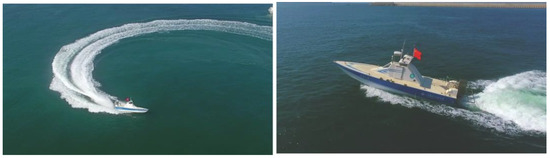
Figure 1.
Unmanned surface vehicle named “Tianxing-1”.
Object detection and tracking are the basis for achieving the autonomous navigation of USVs. The diversity of the object’s information contained in the image determines the result of object detection. The research of USV field-of-view adaption has significance in improving the diversity of object information. The USV will encounter scenes where the object in the image is obscured during navigation. The recognition of the occluded scenes significantly improves the robustness of object tracking. When there are multiple objects in the image, matching the radar-guided object with the object in the image is of interest to improve the stability of object tracking.
1.1. USV Perception System
The USV perception system obtains information about surrounding objects for USVs and is a crucial technology for USVs’ development. The surrounding situational map can be constructed, enabling USVs to understand the current environment. In addition, the perception system is necessary for the safe navigation of USVs. As shown in Figure 2, the USV perception system consists of a perception computer, a marine radar [14,15,16], and a photoelectric device. The CPU model of the perception computer is i7-7700t, and the GPU model is 2080ti. The resolution of the photoelectric visible light sensor is , and the field of view is 1.97 to 40 degrees. The resolution of the infrared sensor is , and the field of view is 2 and 10 degrees. The range of the laser rangefinder is 20 m to 10 km with the error of less than 5 m, the tracking accuracy of the photoelectric servo is 1 mrad, and it can generally navigate in the sea condition of grade 4. The azimuth accuracy of the navigation radar is 0.2 degrees, and the effective detection range is 40 m to 18 km.
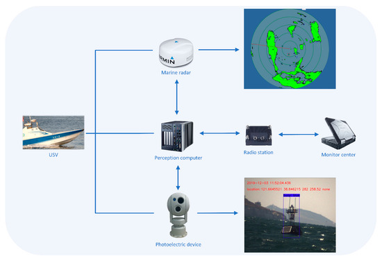
Figure 2.
USV perception system.
Marine radar can obtain object information on distance, direction, speed, and heading. The perception computer consists of a communication module, a radar module, a defogging module, a detection-tracking module, and a decision module. The communication module is used for information transfer between the sensors and the perception computer. The radar module analyzes the object information and removes false objects caused by waves. The defogging module is used to defog the foggy images to improve their quality. The detection-tracking module is used for object detection and object tracking. The decision module determines the process to complete the mission based on the current mission requirements. The photoelectric device consists of a camera sensor and a laser sensor. The image obtained by the camera is essential information for object detection [17,18,19,20]. The laser sensor is used for the precise positioning of the object. The positioning information from laser sensors is more accurate than that from marine radar. As shown in Figure 3, the information transfer diagram of the USV perception system is shown.
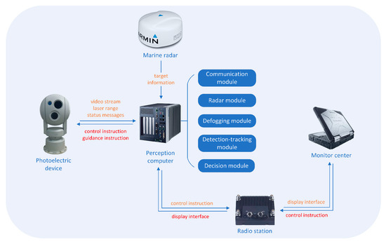
Figure 3.
Information transfer diagram of the USV perception system.
First, the marine radar detects the objects around the USV to obtain the object information. Then, the marine radar sends the object information to the perception computer. The perception computer selects the specified object according to the current demand in the mission and transmits this information to the photoelectric device through control instruction. When the photoelectric device obtains the optical image, the image and state information are sent back to the perception computer. Then, the detection-tracking module detects the object in the image and obtains the pixel coordinates and category of the object. When the photoelectric device has obtained the object information, it controls the motor to track the radar-guided object. Through this process, the real-time dynamic object tracking by the photoelectric device is realized. When the decision module determines that it is in a stable tracking state, the perception computer will send commands to the photoelectric device so that the laser sensor can obtain the precise position information of the object. In addition, the monitor center at the shore can send specific task instructions to the perception computer through the radio station, and the display interface of the perception computer can also be transmitted to the monitor center through the radio station to realize real-time monitoring of the USV.
1.2. Image Edge Detection Algorithm
Edge detection [21,22,23,24] is a fundamental topic in image processing and computer vision. It is one of the most critical aspects of image processing. In a digital image, the area where the image’s grayscale changes drastically is called the edge. Due to the vital position and broad application of edge detection technology in image processing, the research on edge detection has been highly valued by people for many years.
The edge is the boundary of the area where the grayscale changes sharply in the image. There is always an edge between two adjacent areas with different grayscale values, resulting from discontinuous grayscale values. L.G. Roberts proposed a first-order edge detection differential operator that uses the gradient of the image grayscale distribution to characterize the image grayscale change called the Roberts operator [25]. Since then, new theories and methods for edge detection have emerged, such as the Sobel operator [26,27], Kirsh operator, and Prewitt operator [28]. These first-order differential edge detection operators are widely used today because of their slight computational complexity and simple operation. Subsequent refinement processing is generally required when detecting the edge of an image, which will affect the accuracy of edge localization.
It can be known from mathematical theory that the local maximum point of the first-order differential of the function corresponds to the zero-crossing point of the second-order differential, which means that the peak value of the first-order differential can be obtained at the edge point of the image. The cross-section of the second-order differential can be obtained. Therefore, the Laplacian second-order differential edge detection operator was subsequently generated. Compared with the first-order differential edge detection operator, the Laplacian operator [29] is more sensitive to noise and enhances the influence of noise on the detection effect. Based on the above ideas, Hildreth and Marr proposed a second-order edge detection operator that is smoothed and then derived. This operator first smooths the image with a Gaussian function and then uses the isotropic Laplacian operator to derive the image, the zero-crossing point of the second derivative is determined as the edge point, and this operator is also called the Laplacian of Gaussian operator (LOG operator).
Canny proposed three primary criteria for evaluating the performance indicators of edge detection methods and expressed the above three criteria in precise mathematical form for the first time. According to the requirements, the optimal edge detection filter corresponding to a given edge model is obtained by using the optimal numerical analysis method, and the famous Canny operator [30,31] is proposed based on the above theory. Under the influence of Canny’s thought, many similar optimization filter operators were developed later, such as the Deriche operator, Bournnane operator, etc.
1.3. The Content of This Paper and Highlights
When the photoelectric device points to the radar-guided object, there is a case that the features of the radar-guided object are incomplete in the first-frame image. During the navigation of the USV, it may encounter the scene of mast obscuration or green water, which causes the problem of missing objects. When the mast or water blocks the object, the perception system cannot detect the object. In addition, when the photoelectric device points to the object, there may be multiple objects of the same type in the field of view. At this time, the object detection algorithm cannot accurately return the radar-guided object information, resulting in the problem of tracking the wrong object. Therefore, this paper proposes an object extraction algorithm for the first-frame image of unmanned surface vehicles based on a radar-photoelectric system. First, the object’s distance information is obtained by the marine radar. Then, the size of the photoelectric device’s field of view is calculated so that the object can appear in the field of view with a suitable size. According to the pixel size, the field of view is adjusted again. When the scene in the first frame image is identified as the mast obscuration or green water scene, the perception system will stop the subsequent calculations. When multiple objects of the same type appear in the first frame image, the algorithm can stably extract radar-guided objects. The main contributions and organization of this paper can be summarized as the following points:
- 1.
- A field-of-view adaption algorithm is proposed
The field-of-view adaption algorithm adjusts the photoelectric device’s field of view according to the object’s distance and size. When the marine radar obtains the object’s distance information, the perception system calculates the field of view size so that the object can appear in the field of view with a suitable size. Then, according to the object’s pixel size, the secondary field-of-view adjustment is performed so that the object can appear in the field of view with the best size to obtain more detailed information about the object improving the detection accuracy of the local features by 16.8%.
- 2.
- A scene recognition algorithm is proposed
Scene recognition is an algorithm that recognizes the particular scene in the first-frame image. First, the scene recognition algorithm extracts the edge information by the edge detection algorithm and then statistically analyzes the edge information to determine whether the scene is a mast obscuration or green water scene. The perception system will stop the subsequent calculations when the image is detected as these scenes. The algorithm realizes the scene recognition of the first-frame image to improve the robustness of object tracking.
- 3.
- A radar-guided object extraction algorithm is proposed
When the photoelectric device points to the object, there is a case that multiple objects of the same type are in the field of view. At this time, the radar-guided object extraction algorithm analyzes each object in the image and then filters the non-guided objects in the field of view to stably return the radar-guided object information of the first-frame image. The algorithm solves the problem of the unstable extraction of the radar-guided object in multi-object scenes.
In the second section of the paper, we analyze the imaging principle of the object and propose a field-of-view adaptive algorithm. The algorithm is realized by means of two field-of-view adaptations. In the third section of the paper, we analyze the image characteristics of the mast obscuration and green-water scene. For this feature, we propose the scene recognition algorithm. The algorithm realizes the scene recognition of the first-frame image to improve the robustness of object tracking. In the fourth section of the paper, we analyze the case of multiple objects within the same field of view and propose a radar-guided object extraction algorithm. The algorithm solves the problem of the unstable extraction of the radar-guided object in multi-object scenes.
2. Field-of-View Adaption Algorithm
The field-of-view adaption algorithm is an algorithm that adaptively adjusts the field of view of the photoelectric device according to the object’s distance and size. After the photoelectric device obtains the information of the radar-guided object, the photoelectric device calculates the longitude and latitude information of the object to obtain the azimuth information. The photoelectric device rotates, and the radar-guided object appears in the field of view. After the marine radar obtains the distance information of the object, the perception system calculates the field of view so that the object can appear in the field of view with a suitable size. Then, according to the pixel size of the object, the secondary field-of-view adjustment is performed so that the object can appear in the field of view with the best size to obtain more detailed information about the object. The algorithm can ensure the stability of USVs in various missions. As shown in Figure 4, it is a schematic diagram of the relative position of the USV and the object. The marine radar detects the surrounding environment and can obtain the distance information of the target and the azimuth of the target.
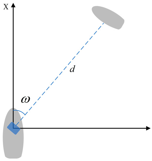
Figure 4.
Relative position of the USV and the object.
As shown in Figure 5, it is a schematic diagram of the USV’s field of view. The field of view is , the field of view occupied by the object is , the actual width of the image on the plane where the object is located is , the pixel width of the image is , the actual width of the object in the image is , and the pixel width of the object is . In addition, the field-of-view adaptation coefficient is . The adaptation coefficient is the basis for adjusting the size of the field of view, which can be expressed as:
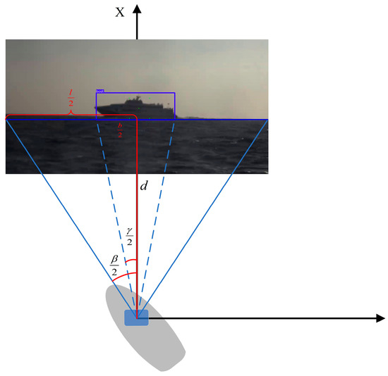
Figure 5.
Schematic diagram of the USV’s field of view.
The object distance information obtained by the marine radar is , the estimated object size information is , and the adaptation coefficient is .
Based on the above information, the expected field of view is calculated as follows:
By the above calculation, the expected field of view can be obtained so that the object can appear in the field of view at a suitable size after the photoelectric device points to the object, and the pixel width of the object can be obtained. At this time, the precise distance of the object can be obtained by the laser sensor. The size of the actual width of the object can be obtained by calculation, and the calculation process is as follows:
Since there are significant errors in the object distance information and object size information obtained by the maritime radar, a secondary field-of-view adaption adjustment is required to make the object appear in the field of view with the best size to ensure that the perception system obtains the best visual information of the object. The first adaption field-of-view adjustment is based on the object’s information obtained from the marine radar, while the second adaption field-of-view adjustment is based on the object’s pixel size in the image.
In the secondary field-of-view adaption algorithm, the expected field of view of the photoelectric device is , the field of view occupied by the object is , the actual width of the image on the plane where the object is located is , and the pixel width of the image is . The actual width of the object is , the pixel width of the object is , and the object distance measured by the laser sensor is . In addition, the adaption coefficient in the secondary field-of-view adaption algorithm is , which can be expressed as:
Based on the above information, the expected field of view is calculated as follows:
The expected field of view can be obtained through the above calculation so that the object can appear in the field of view with the best size. As shown in Figure 6, it is a schematic diagram of the secondary field-of-view adaption algorithm of the USV.
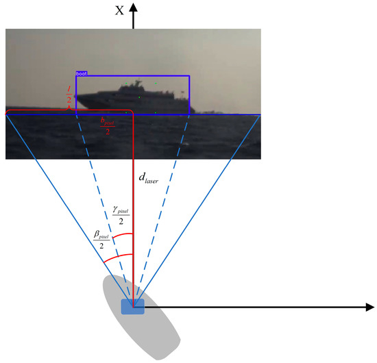
Figure 6.
Secondary field-of-view adaption algorithm of the USV.
Ten different maritime test environments are selected to test the field-of-view adaptive algorithm. Comparing the first frame without field-of-view adaptive processing with the image with field-of-view adaptive processing shows that the object’s local feature detection accuracy is improved by 16.8%.
3. Scene Recognition Algorithm
The scene recognition is an algorithm for the perception system to recognize the special scenes in the first frame image. After the photoelectric device has pointed to the object, the scene can be classified as follows, according to the characteristics of the image. The first is the single-object scene, where only the radar-guided object is in the image. The second is the different kind of multi-object scene, in which there are multiple objects but in different categories. The third is the multi-object scene of the same category. In this scene, there are multiple objects in the same category. The fourth is the green-water scene, where the water blocks the object. The fifth is the mast-obscuration scene, where the mast occludes the object. The perception system cannot identify and detect the object if the scene is the green-water scene or the mast-obscuration scene.
3.1. Recognition of the Mast-Obscuration Scene
The radar-guided object, the mast of the USV, and the photoelectric device are in a straight line when the scene of the first frame image is the mast-obscuration scene. As shown in Figure 7, it is the images of the mast-obscuration scene. The perception system cannot identify and detect the object when the scene is the mast-obscuration scene.
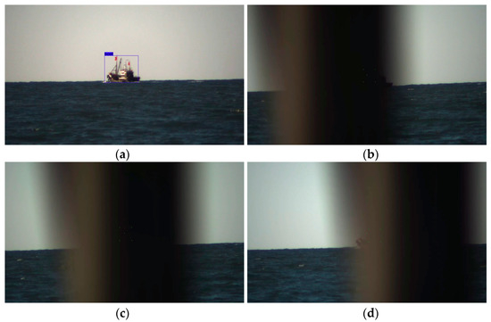
Figure 7.
Images of the mast-obscuration scene: (a) A scene before the object is obscured; (b) The scene 1 where the object is obscured; (c) The scene 2 where the object is obscured; (d) The scene 3 where the object is obscured.
There is an area where the sky area, the sea–sky line, and the sea area are all occluded, analyzing the mast-obscuration scene. In addition, the image gradient of the particular area is slight. The edge of the image can be detected according to the image gradient characteristics of the region. We determine whether it is a mast-obscuration scene, according to the edge detection result.
The Prewitt operator is an edge detection algorithm based on the first-order differential operator. The algorithm uses the grayscale difference between the upper and lower pixels and the grayscale difference between the left and right adjacent points to extract the edge information in the image. The principle is to use two directional templates to perform neighborhood convolution with the image; one template is used to detect horizontal edges, and another is used to detect vertical edges. Since the purpose of edge detection is not to obtain accurate object’s edge information, the Prewitt operator edge detection algorithm can ensure the edge extraction effect and meet the perception system’s real-time requirements.
Image is the grayscale image of the first frame image, and is the grayscale value at in image . and are the approximate values of the horizontal and vertical grayscale partial derivatives, respectively. The mathematical expressions are as follows:
After the above calculation, the approximate value of the horizontal gray partial derivative and the approximate value of each pixel’s vertical gray partial derivative can be obtained. Gradients in two directions can be obtained for each pixel. The following formula calculates an approximation of the gradient:
When the gradient is greater than the gradient threshold , the pixel is determined to be a bright spot, and the original gray value of the pixel is retained. When the gradient is less than or equal to the gradient threshold , the pixel is determined to be a dark point, and the gray value at this pixel is zero. Through the above determination, an edge-detected image is obtained. As shown in Figure 8, it is the edge detection result of the mast-obscuration scene.
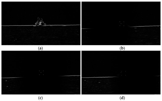
Figure 8.
Edge detection result of the mast-obscuration scene: (a) A scene before the object is obscured; (b) The scene 1 where the object is obscured; (c) The scene 2 where the object is obscured; (d) The scene 3 where the object is obscured.
The analysis of the edge detection result shows that the sea–sky line appears to be interrupted due to mast occlusion. In addition, the sea region under the mast occlusion has no sea noise information. According to the above image features, this paper segments the image horizontally and counts the number of bright spots within each region. As shown in Figure 9, a schematic diagram of the image segmentation is shown.
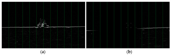

Figure 9.
Schematic diagram of the image segmentation: (a) A scene before the object is obscured; (b) The scene 1 where the object is obscured; (c) The scene 2 where the object is obscured; (d) The scene 3 where the object is obscured.
The image above shows that the number of bright spots in the segmented area occluded by the mast is significantly smaller than that in the segmented area not obscured by the mast. is the edge detection image, the resolution of image is , and is the serial number of the segmented area in image . is the number of bright spots in the segmented area, is the horizontal coordinate of the pixel in the image , is the vertical coordinate of the pixel in the image , and is the left critical value of the segmented area in the direction. The function is the bright spot determination function, is the gray level of the pixel at in image , and is the determination threshold in the bright spot determination function. The calculation process is as follows:
By the above calculation, the number of bright spots in each segmentation region in the image can be obtained. As shown in Figure 10, the statistical curves of the bright spots in the segmented regions are shown.
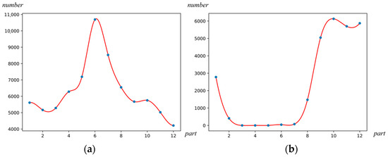
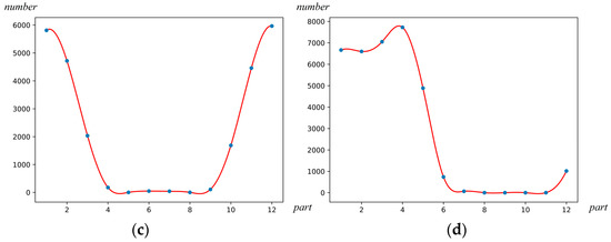
Figure 10.
Statistical curves of the bright spots in the segmented regions: (a) A scene before the object is obscured; (b) The scene 1 where the object is obscured; (c) The scene 2 where the object is obscured; (d) The scene 3 where the object is obscured.
The above curves show that there is no segmented area with less than 100 bright spots in the scene not blocked by the mast and multiple divided areas with less than 100 bright spots in the statistical result of the scene blocked by the mast. is the decision function of the mast-obscuration scene, is the number of bright spots in the segmented area in the statistics, and is the judgment threshold in the decision function of the mast-obscuration scene. is the number of the mast-obscuration areas, and is the number of the segmented areas. The calculation process is as follows:
is the ratio of the number of mast occlusion areas to the total number of divided areas, is the judgment result of the mast-obscuration scene, and is the judgment threshold of the mast-obscuration scene. If the ratio is less than the determination threshold , the determination result is equal to 0, and the scene is determined to be a non-mast-obscuration scene; if the ratio is greater than or equal to the determination threshold , the determination result is equal to 1, and the scene is determined to be a mast-obscuration scene. The expression is as follows:
3.2. Recognition of the Green-Water Scene
The radar-guided object is obscured by water when the scene of the first frame image is the green-water scene. As shown in Figure 11, it is the image of the green-water scene. The perception system cannot identify and detect the object when the scene is the green-water scene.
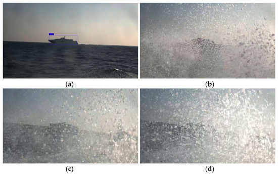
Figure 11.
Images of the green-water scene: (a) A scene before the object is obscured; (b) The scene 1 where the object is obscured; (c) The scene 2 where the object is obscured; (d) The scene 3 where the object is obscured.
The camera of the photoelectric device is covered by water, analyzing the green-water scene. For the non-green-water wave scene, the edge information of the sky part above the sea–sky line in the image is little, while for the green-water scene, the edge information of that increases significantly. So, it is determined whether it is a green-water scene by the edge detection result. Laplacian edge detection is an edge detection algorithm that uses a second derivative to extract image edge information. The Laplacian operator is an isotropic operator. Isotropic operator means that the use of one operator can sharpen borders and lines in any direction without directionality. Like the Sobel and Prewitt operators, they use different operators to extract edges in different directions. Isotropy is the advantage of the Laplacian operator that distinguishes it from other first-order differential operators. The Laplacian operator for the grayscale image in the first frame can be defined as:
For a two-dimensional discrete image, the following calculation can be used as an approximation to the second-order partial differential:
Therefore, the expression of the Laplacian operator is:
According to the above expression, the following filter template can be obtained:
When convolving the image with the Laplacian operator, if the absolute value of the response is greater than the threshold , the pixel is determined to be a bright spot, and the original gray value of the pixel is retained. If the absolute value of the response is less than or equal to the threshold value , it is determined that the pixel is a dark point, and the gray value of the pixel is zero. Through the above determination, an edge-detected image is obtained. As shown in Figure 12, it is the edge detection result of the green-water scene.
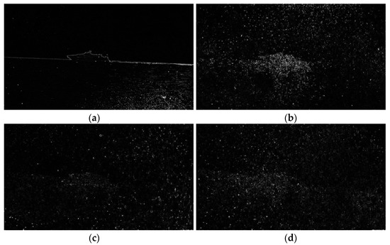
Figure 12.
Edge detection result of the green-water scene: (a) A scene before the object is obscured; (b) The scene 1 where the object is obscured; (c) The scene 2 where the object is obscured; (d) The scene 3 where the object is obscured.
For the non-green-water wave scene, the edge information of the sky part above the sea–sky line in the image is little, while for the green-water scene, the edge information of that increases significantly. Therefore, this paper divides the image vertically and counts the number of bright spots in each area according to the above image characteristics. As shown in Figure 13, it is a schematic diagram of the vertical region segmentation of the image.
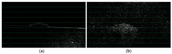

Figure 13.
Schematic diagram of the image segmentation: (a) A scene before the object is obscured; (b) The scene 1 where the object is obscured; (c) The scene 2 where the object is obscured; (d) The scene 3 where the object is obscured.
is the image obtained after edge detection, and the resolution of image is . is the serial number of the segmented area in image , and is the number of bright spots in the segmented area. is the horizontal coordinate of the pixel in image , is the vertical coordinate of the pixel in image , is the left critical value of the segmented area in the direction, and the function is the bright spot determination function. is the pixel’s gray level at in image , and is the decision threshold of the bright spot determination function. The calculation process is as follows:
By the above calculation, we can obtain the number of bright spots in each segmented area in the image. As shown in Figure 14, it is the statistical curves of bright spots in the segmented regions.
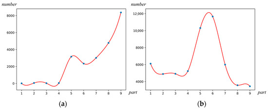

Figure 14.
Statistical curves of the bright spots in the segmented regions: (a) A scene before the object is obscured; (b) The scene 1 where the object is obscured; (c) The scene 2 where the object is obscured; (d) The scene 3 where the object is obscured.
The above curves show that there is no segmented area with less than 100 bright spots in the green-water scene and multiple divided areas with less than 100 bright spots in the non-green-water scene. is the decision function of the green-water scene, is the number of bright spots in the segmented area in the statistics, is the judgment threshold in the decision function of the mast-obscuration scene, is the number of the mast-obscuration areas, and is the number of the segmented areas. The calculation process is as follows:
is the ratio of the number of mast occlusion areas to the total number of divided areas, is the judgment result of the mast-obscuration scene, and is the judgment threshold of the mast-obscuration scene. If the ratio is less than the determination threshold , the determination result is equal to 0, and the scene is determined to be a non-green-water scene. If the ratio is greater than or equal to the determination threshold , the determination result is equal to 1, and the scene is determined to be a green-water scene. The expression is as follows:
4. Radar-Guided Object Extraction Algorithm
Real-time object tracking by the perception system is an essential part of dynamic object tracking of the USV. The above process includes three parts: First, the marine radar detects the object and guides the photoelectric device to complete the object pointing. Second, the perception computer performs object detection on the sequence images returned by the photoelectric device. Third, the photoelectric device realizes object tracking according to the object’s position and performs laser positioning on the object.
Depending on the type and number of objects in the field of view, scenes can be classified into single-object scenes, different kinds of multi-object scenes, and the same kind of multi-object scenes. If there is only a single object in the field of view, the perception computer can obtain the pixel coordinates of the object through the object detection algorithm and obtain the off-target distance of the object. The resolution of the first frame image is , and the bullseye coordinate of the image is ; then, the off-target amount of the object can be expressed as follows:
After the photoelectric device has pointed to the object, if there are multiple objects of the same type in the field of view, the object detection algorithm cannot accurately obtain the position of the radar-guided object. The paper proposes a radar-guided object extraction algorithm, which can filter non-guided objects. The proposed algorithm improves the robustness of object tracking and enables the perception system to achieve a stable return of the radar-guided object distance in the first frame image even in a complex environment. Although the object distance error obtained by the marine radar is relatively large, the object azimuth information is relatively accurate. Therefore, the radar-guided objects are located in the middle region of the image. Based on the above characteristics, the objects outside the region of interest (ROI) can be filtered, and the interference of other objects with the returned results can be reduced.
is the maximum deviation angle of the object detected by the marine radar. is the field-of-view angle of the photoelectric device, and the resolution of the first frame image is . is the maximum deviation of the actual pixel position of the object in the horizontal direction. is the fault tolerance parameter of the ROI. is the minimum critical value of the ROI. is the maximum critical value of the ROI. The expression is as follows:
In this case, several objects of the same category are in the ROI. According to the position of each object in the horizontal direction, the following calculation is performed.
is the serial number of each object in the ROI of the first frame image. is the horizontal pixel coordinate of object , and is the distance between the object and the center of the image in the horizontal direction. is the number of objects in the ROI of the image, and is a parameter for sorting. is the new serial number of the object . The calculation process is as follows:
The above calculation shows each object’s new serial number in the ROI of the first frame image. However, when two objects of the same type are located on both sides of the image centerline, and the absolute values of the two objects are close, the radar-guided object cannot be stably extracted. Therefore, this paper performs correlation calculations on the objects’ position in adjacent frames.
is the off-target distance in the horizontal direction and is the off-target distance in the vertical direction. is the associated flag of two adjacent frames. The calculation process is as follows:
If is 0 or 1, it means that the object correlates with the object of the previous frame; if is −1, it means that the object has no correlation with the object of the previous frame, and the object selection result of the previous frame is retained. Estimate the object’s pixel size based on the distance and category. According to the estimated pixel size, the objects in the ROI are screened again to obtain the final radar-guided object.
is the function of object screening. is the object serial number retained after screening, is the object pixel width, and is the object pixel height. is the object pixel area, and is the number of objects reserved for screening. The calculation process is as follows:
This paper tests the radar-guided object extraction algorithm in the case of multiple buoys in a simple background, the case of multiple buoys in a complex background, and the case of multiple ships in a simple and the case of multiple ships in the complex background.
As shown in Figure 15a, it is the test of the radar-guided object extraction algorithm in the case of multiple buoys in simple background. In the same field of view, there are two objects of the same type. After the marine radar detection, according to the mission requirements, the decision module autonomously selects the object closest to the USV. In this image, the green buoy is the object guided by the radar, and the red buoy is successfully filtered out. As shown in Figure 15b, it is the test of the radar-guided object extraction algorithm in the case of multiple buoys in a complex background. The background behind the buoy is complicated. During the test, the red buoys was successfully filtered out.
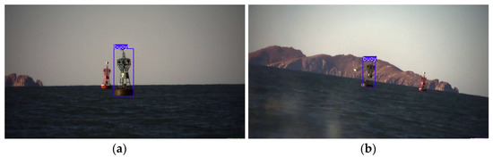
Figure 15.
Extraction results for the multi-buoy case: (a) Test results in a simple background; (b) Test results in a complex background.
As shown in Figure 16a, it is the test of the radar-guided object extraction algorithm in the case of multiple ships in the simple background. In the same field of view, there are two objects of the same type. After the marine radar detection, according to the mission requirements, the decision module autonomously selects the object closest to the USV. In this image, the ship in the middle is the object guided by the radar, and another ship is successfully filtered out. As shown in Figure 16b, it is the test of the radar-guided object extraction algorithm in the case of multiple ships in a complex background. The background behind the ships is complicated. During the test, another ship is successfully filtered out.

Figure 16.
Extraction results for the multi-ship case: (a) Test results in a simple background; (b) Test results in a complex background.
As shown in Figure 17, it is the flow chart of the USV object tracking. The part marked with an asterisk is the main research content of this paper.
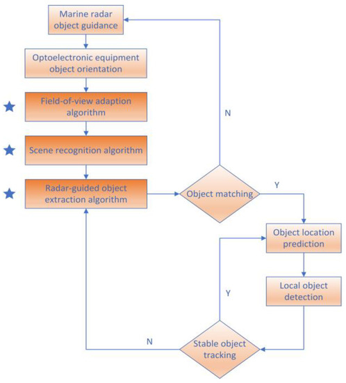
Figure 17.
Flow chart of the USV object tracking.
5. Conclusions
When the photoelectric device points to the radar-guided object, there is a case that the object’s pixel size in the first-frame image is not suitable, resulting in missing object information. During the navigation of the USV, it may encounter the scene of mast obscuration or green water. When the mast or water blocks the object, the perception system cannot detect the object. In addition, when the photoelectric device points to the object, there may be multiple objects of the same type in the field of view. At this time, the object detection algorithm cannot accurately return the radar-guided object information, resulting in the problem of tracking the wrong object. Therefore, this paper proposes an object extraction algorithm for the first-frame image of unmanned surface vehicles based on a radar-photoelectric system.
The first is the field-of-view adaption algorithm. The algorithm adjusts the photoelectric device’s field of view according to the object’s distance and size. When the marine radar obtains the object’s distance information, the perception system calculates the field of view size so that the object can appear in the field of view with a suitable size. Then, according to the object’s pixel size, the secondary field-of-view adjustment is performed so that the object can appear in the field of view with the best size to obtain more detailed information about the object. The second is the scene recognition algorithm. The algorithm recognizes the particular scene in the first-frame image. First, the scene recognition algorithm extracts the edge information by the edge detection algorithm and then statistically analyzes the edge information to determine whether the scene is a mast obscuration or green water scene. The perception system will stop the subsequent calculations when the image is detected as these scenes. The third is the radar-guided object extraction algorithm. When the photoelectric device points to the object, there is a case that multiple objects of the same type are in the field of view. At this time, the radar-guided object extraction algorithm analyzes each object in the image and then filters the non-guided objects in the field of view to stably return the radar-guided object information of the first-frame image.
Author Contributions
Conceptualization, Q.Y.; methodology, Q.Y.; software, Q.Y.; validation, Q.Y. and Y.S.; formal analysis, Q.Y and R.Z.; investigation, Q.Y.; resources, Q.Y.; data curation, Q.Y. and R.Z.; writing—original draft preparation, Q.Y.; writing—review and editing, Q.Y.; visualization, Q.Y.; supervision, Y.S.; project administration, Y.S.; funding acquisition, Y.S. All authors have read and agreed to the published version of the manuscript.
Funding
This research received no external funding.
Institutional Review Board Statement
Not applicable.
Acknowledgments
The authors are grateful to the anonymous reviewers and editors for their suggestions and assistance in significantly improving the manuscript.
Conflicts of Interest
The authors declare no conflict of interest.
References
- Breivik, M.; Hovstein, V.E.; Fossen, T.I. Straight-Line Target Tracking for Unmanned Surface Vehicles. Model. Identif. Control 2008, 29, 131–149. [Google Scholar] [CrossRef]
- Liu, Z.; Zhang, Y.; Yu, X.; Yuan, C. Unmanned Surface Vehicles: An Overview of Developments and Challenges. Annu. Rev. Control 2016, 41, 71–93. [Google Scholar] [CrossRef]
- Wang, N.; Zhang, Y.; Ahn, C.K.; Xu, Q. Autonomous Pilot of Unmanned Surface Vehicles: Bridging Path Planning and Tracking. IEEE Trans. Veh. Technol. 2022, 71, 2358–2374. [Google Scholar] [CrossRef]
- Wang, N.; Gao, Y.; Zhao, H.; Ahn, C.K. Reinforcement Learning-Based Optimal Tracking Control of an Unknown Unmanned Surface Vehicle. IEEE Trans. Neural Netw. Learn. Syst. 2021, 32, 3034–3045. [Google Scholar] [CrossRef] [PubMed]
- Stateczny, A.; Burdziakowski, P.; Najdecka, K.; Domagalska-Stateczna, B. Accuracy of Trajectory Tracking Based on Nonlinear Guidance Logic for Hydrographic Unmanned Surface Vessels. Sensors 2020, 20, 832. [Google Scholar] [CrossRef]
- Stateczny, A.; Gierlowski, K.; Hoeft, M. Wireless Local Area Network Technologies as Communication Solutions for Unmanned Surface Vehicles. Sensors 2022, 22, 655. [Google Scholar] [CrossRef]
- USV Compliant Obstacle Avoidance Based on Dynamic Two Ship Domains | Elsevier Enhanced Reader. Available online: https://reader.elsevier.com/reader/sd/pii/S0029801822015645?token=A50F4FA088F3AA07183A148DB9BAE38974C407A28C37F980A2134CC9B667546056A60E54DF9133593FC2F370F5D422C9&originRegion=us-east-1&originCreation=20221023072530 (accessed on 23 October 2022).
- Ciaparrone, G.; Luque Sánchez, F.; Tabik, S.; Troiano, L.; Tagliaferri, R.; Herrera, F. Deep Learning in Video Multi-Object Tracking: A Survey. Neurocomputing 2020, 381, 61–88. [Google Scholar] [CrossRef]
- Liu, Q.; Li, X.; He, Z. Learning Deep Multi-Level Similarity for Thermal Infrared Object Tracking. IEEE Trans. Multimed. 2020, 23, 2114–2126. [Google Scholar] [CrossRef]
- Luo, W.; Xing, J.; Milan, A.; Zhang, X.; Liu, W.; Kim, T.-K. Multiple Object Tracking: A Literature Review. Artif. Intell. 2021, 293, 103448. [Google Scholar] [CrossRef]
- Sun, S.; Akhtar, N.; Song, H.; Mian, A.S.; Shah, M. Deep Affinity Network for Multiple Object Tracking. IEEE Trans. Pattern Anal. Mach. Intell. 2019, 43, 104–119. [Google Scholar] [CrossRef]
- Bruzzone, G.; Bruzzone, G.; Bibuli, M.; Caccia, M. Autonomous Mine Hunting Mission for the Charlie USV. In Proceedings of the 2011 Ieee—Oceans Spain, Santander, Spain, 6–9 June 2011; IEEE: New York, NY, USA. [Google Scholar]
- Ohta, Y.; Yoshida, H.; Ishibashi, S.; Sugesawa, M.; Fan, F.H.; Tanaka, K. Seabed Resource Exploration Performed by AUV “Yumeiruka”. In In Proceedings of the Oceans 2016 Mts/Ieee Monterey, Monterey, CA, USA, 19–23 September 2016; IEEE: New York, NY, USA. [Google Scholar]
- Chen, X.; Huang, W. Identification of Rain and Low-Backscatter Regions in X-Band Marine Radar Images: An Unsupervised Approach. Ieee Trans. Geosci. Remote Sens. 2020, 58, 4225–4236. [Google Scholar] [CrossRef]
- Zhuang, J.; Zhang, L.; Zhao, S.; Cao, J.; Wang, B.; Sun, H. Radar-Based Collision Avoidance for Unmanned Surface Vehicles. China Ocean Eng. 2016, 30, 867–883. [Google Scholar] [CrossRef]
- Stateczny, A.; Kazimierski, W.; Gronska-Sledz, D.; Motyl, W. The Empirical Application of Automotive 3D Radar Sensor for Target Detection for an Autonomous Surface Vehicle’s Navigation. Remote Sens. 2019, 11, 1156. [Google Scholar] [CrossRef]
- Redmon, J.; Divvala, S.; Girshick, R.; Farhadi, A. You Only Look Once: Unified, Real-Time Object Detection. In Proceedings of the 2016 Ieee Conference on Computer Vision and Pattern Recognition (CVPR), Las Vegas, NV, USA, 27–30 June 2016; IEEE: New York, NY, USA; pp. 779–788. [Google Scholar]
- Redmon, J.; Farhadi, A. YOLOv3: An Incremental Improvement 2018. arXiv 2018, arXiv:1804.02767. [Google Scholar]
- Ren, S.; He, K.; Girshick, R.; Sun, J. Faster R-CNN: Towards Real-Time Object Detection with Region Proposal Networks. arXiv 2016, arXiv:1506.01497. [Google Scholar]
- Xu, Y.; Fu, M.; Wang, Q.; Wang, Y.; Chen, K.; Xia, G.-S.; Bai, X. Gliding Vertex on the Horizontal Bounding Box for Multi-Oriented Object Detection. IEEE Trans. Pattern Anal. Mach. Intell. 2021, 43, 1452–1459. [Google Scholar] [CrossRef]
- Li, X.; Jiao, H.; Wang, Y. Edge Detection Algorithm of Cancer Image Based on Deep Learning. Bioengineered 2020, 11, 693–707. [Google Scholar] [CrossRef]
- Mittal, M.; Verma, A.; Kaur, I.; Kaur, B.; Sharma, M.; Goyal, L.M.; Roy, S.; Kim, T.-H. An Efficient Edge Detection Approach to Provide Better Edge Connectivity for Image Analysis. IEEE Access 2019, 7, 33240–33255. [Google Scholar] [CrossRef]
- Orujov, F.; Maskeliunas, R.; Damasevicius, R.; Wei, W. Fuzzy Based Image Edge Detection Algorithm for Blood Vessel Detection in Retinal Images. Appl. Soft Comput. 2020, 94, 106452. [Google Scholar] [CrossRef]
- Versaci, M.; Morabito, F.C. Image Edge Detection: A New Approach Based on Fuzzy Entropy and Fuzzy Divergence. Int. J. Fuzzy Syst. 2021, 23, 918–936. [Google Scholar] [CrossRef]
- Tao, J.; Cai, J.; Xie, H.; Ma, X. Based on Otsu Thresholding Roberts Edge Detection Algorithm Research. In Proceedings of the 2nd International Conference on Information, Electronics and Computer; Jin, J.X., Bhattacharyya, D., Eds.; Atlantis Press: Paris, France, 2014; Volume 59, pp. 121–124. [Google Scholar]
- Chetia, R.; Boruah, S.M.B.; Sahu, P.P. Quantum Image Edge Detection Using Improved Sobel Mask Based on NEQR. Quantum Inf. Process. 2021, 20, 21. [Google Scholar] [CrossRef]
- Ravivarma, G.; Gavaskar, K.; Malathi, D.; Asha, K.G.; Ashok, B.; Aarthi, S. Implementation of Sobel Operator Based Image Edge Detection on FPGA. In Materials Today-Proceedings; Elsevier: Amsterdam, The Netherlands, 2021; Volume 45, pp. 2401–2407. [Google Scholar]
- Ye, H.; Shen, B.; Yan, S. Prewitt Edge Detection Based on BM3D Image Denoising. In Proceedings of the 2018 Ieee 3rd Advanced Information Technology, Electronic and Automation Control Conference (IAEAC 2018), Chongqing, China, 12–14 October 2018; Xu, B., Ed.; IEEE: New York, NY, USA, 2018; pp. 1593–1597. [Google Scholar]
- Wang, X. Laplacian Operator-Based Edge Detectors. Ieee Trans. Pattern Anal. Mach. Intell. 2007, 29, 886–890. [Google Scholar] [CrossRef] [PubMed]
- Gaurav, K.; Ghanekar, U. Image Steganography Based on Canny Edge Detection, Dilation Operator and Hybrid Coding. J. Inf. Secur. Appl. 2018, 41, 41–51. [Google Scholar] [CrossRef]
- Kanchanatripop, P.; Zhang, D. Adaptive Image Edge Extraction Based on Discrete Algorithm and Classical Canny Operator. Symmetry 2020, 12, 1749. [Google Scholar] [CrossRef]


Disclaimer/Publisher’s Note: The statements, opinions and data contained in all publications are solely those of the individual author(s) and contributor(s) and not of MDPI and/or the editor(s). MDPI and/or the editor(s) disclaim responsibility for any injury to people or property resulting from any ideas, methods, instructions or products referred to in the content. |
© 2023 by the authors. Licensee MDPI, Basel, Switzerland. This article is an open access article distributed under the terms and conditions of the Creative Commons Attribution (CC BY) license (https://creativecommons.org/licenses/by/4.0/).