Abstract
Autonomous underwater vehicles (AUVs) are increasingly being used in missions involving submarine cable detection, underwater archaeology, pipeline inspection, military reconnaissance, and so on. It is very important to realize AUV path tracking to accomplish these missions. In this paper, a fuzzy controller based on the established kinematic and dynamic models of AUV systems is presented to solve the AUV path-tracking problem. In order to design the fuzzy controller to exhibit good performance, we select the path length, smoothness, and cross-track position error as the multiple optimization performance indexes for the fuzzy controller. We propose the particle swarm optimization (PSO) algorithm to determine the parameters of the membership functions. Different scenarios are presented to test the performance of the proposed algorithm, including the straight line, sine curve, half-moon shape, Archimedean spiral, and practical paths. The results are given to illustrate the effectiveness and feasibility of the fuzzy controller with the optimization of multiple performance indexes.
1. Introduction
The ocean is an important strategic space for economic and social development. Due to the increasing exploitation and utilization of marine resources, autonomous underwater vehicles (AUVs) have been rapidly developed for use in the fields of pipeline inspection, seawater quality detection, marine geological exploration, submarine cable detection, and so on [1,2,3]. It is important to control the AUV to complete missions quickly and accurately [4,5,6]; however, complex underwater working environments increase the difficulty of controlling AUVs [7]. Therefore, as the premise to realize AUV missions, path tracking becomes an important problem to be solved.
There has been much research on AUV path tracking based on traditional design methods, including proportional integral differential (PID) control [8,9], sliding mode control [10,11], predictive control [12], and so on. PID is one of the most widely used algorithms for controller design; to guide an AUV to track an underwater cable, it forms a straight-line path-tracking control problem with magnetic sensing. Previous research presented a PID controller to track the desired guidance profiles in light of the linearizing feedback method [8]. The PID algorithm can give a line-of-sight guidance law with drift angle compensation to solve the problem of AUV tracking in a complex marine environment, and the PID algorithm can be used to guide AUVs to track the desired path [9]. However, PID is a linear control method, which is difficult to use in complex nonlinear systems related to AUVs in practice. To solve the under-actuated AUV horizontal path-tracking control problem, the authors of another study utilized a sliding mode control method with line-of-sight guidance and cross-track errors [10]; however, chattering was inevitable in the tracking control process. This necessitated a nonlinear second-order sliding mode controller for the purpose of improving the stability of the control system by eliminating the chattering motion [11]. In light of the backstepping algorithm, a model predictive control method was given for AUV path tracking [12]. In summary, the above traditional methods [8,9,10,11,12] are highly dependent on the models of AUV control systems, which are difficult to apply in engineering practice because of the difficulty of obtaining accurate models in complex underwater environments.
Compared with the traditional control methods of path tracking, intelligent algorithms have attracted more and more attention because their application of intelligent control is independent of an accurate kinetic model. Reinforcement learning refers to agent learning according to “trial and error”, which interacts with the environment to obtain rewards to guide behavior for path tracking [13,14]. A line-of-sight method of guidance was proposed by reinforcement learning algorithms, which can also utilize long short-term memory neural networks to pre-train the reinforcement learning framework to speed up the learning process [13]. Considering the uncertainty of ocean currents and according to the data on ocean currents obtained by the observer, one study presented a novel reward function to improve the learning ability of a reinforcement learning architecture, and thus, deep reinforcement learning was developed for path tracking [14]. Fuzzy control is a method considering the theory of fuzzy mathematics, which has been used for AUV path tracking [15,16,17]. In fuzzy control, a nonlinear single-input fuzzy controller was used for path tracking, resulting in reductions in the computation complexity [15]. For an AUV with an unknown actuator saturation and environmental disturbance, the authors of one study presented a kinematic controller by the backstepping technique, whose law was designed in light of an indirect adaptive fuzzy logic control system [16]. To improve the performance of fuzzy controllers, the authors of another study proposed a fuzzy controller optimized by the genetic algorithm [17]. In summary, although there are many different intelligent control methods for AUV path tracking, they are focused on improving the tracking error; in practice, the path length and smoothness are also important for path-tracking performance. Therefore, a new method is needed to solve the AUV path-tracking problem with multiple good performance indexes.
It should be noted that the existing fuzzy theory and the related research have made some contributions regarding the collision avoidance problem in marine engineering. In one study, fuzzy theory was used to reason the degree of the collision risk, A*search was used to make an avoidance action plan, and the action space searched by the ship was formed in the expert system using marine traffic rules [18]. In order to trigger the prompt alert of a potential collision, the authors of another study utilized evidential research theory to calculate the risk of collision according to the relevant navigation information [19]. Based on the need to prevent collisions according to sea rules, the authors of another study proposed a collision risk inference system using fuzzy rules to enable autonomous surface ships to avoid collisions [20]. Furthermore, on the basis of [20], the authors of another study proposed a local route planning method to avoid collisions with maritime autonomous surface ships [21]. Although the above works can provide some reference to fuzzy theory [18,19,20,21], they are difficult to directly use in AUV path tracking.
Path tracking is very important to perform missions in complex underwater environments. To solve the path-tracking problem for AUVs according to the established kinematic and dynamic models, a fuzzy controller is presented to realize path tracking. We select the path length, smoothness and cross-track position error as the performance indexes for the fuzzy controller, which determines the AUV tracking path energy, traveling time and tracking accuracy. The fuzzy controller is optimized with the optimization of membership function by the particle swarm optimization (PSO) algorithm. The designed fuzzy controller makes a path-tracking system with strong robustness and anti-interference ability.
The rest of this paper is arranged as follows. Section 2 gives the problem description and definition for AUV path tracking; Section 3 presents mathematical models for AUV path tracking; Section 4 proposes a fuzzy control method based on the PSO algorithm for AUV path tracking; Section 5 gives the results and discussion for the proposed algorithm; Section 6 provides some conclusive remarks.
2. Problem Description and Definition for AUV Path Tracking
The goal of AUV path tracking is to follow the desired path with the performance indexes. In the tracking process, once the coordinates of the current and target locations are given, the desired attitude angles can be obtained with the desired AUV velocity, the essence is to eliminate the error between the practical and desired angles. In order to solve the AUV path-tracking problem, we select the path length, smoothness and cross-track position error as the path-tracking performance indexes. The reason is that the indexes determine the path tracking energy consumption, travelling time, etc. [22]. The fuzzy control can solve the control problem of nonlinear system with strong robustness effectively; therefore, the fuzzy controller is presented for path tracking in this paper. Figure 1 gives the technology roadmap for AUV path tracking. The optimization performances for the fuzzy controller are formed according to the established kinematic and dynamic models, the deviations and their derivatives are taken as input parameters. We present the PSO algorithm to optimize the membership function to realize optimal path tracking. The AUV tracks with the desired path based on the optimized fuzzy controller.

Figure 1.
The technology roadmap for AUV path tracking.
We select the cross-track position and heading angle errors as the important factors to illustrate the path-tracking effect [10]. Figure 2 shows the definitions of the AUV’s cross-track position and heading angle errors, where , and are the adjacent discrete points of the desired path. is the AUV’s center.
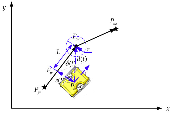
Figure 2.
Cross-track position and heading angle errors for the AUV.
The cross-track position error is the vertical distance from the AUV’s center to the adjacent segment of the desired path. In light of the points , and , the cross-track position error can be obtained as follows:
where is the distance from the AUV’s center to the target point.
The cross-track heading angle error is an angle between the and vectors, which can be given as follows:
In this paper, the smaller the cross-track position and heading angle errors, the better the tracking effect.
In Figure 2, the straight line is perpendicular to , is the corresponding crossing point. Whether the AUV drives into the next segment path can be evaluated by the following decision factor :
where denotes the length of straight line . and are the circle radius and center, respectively. If or , then , that is, the AUV executes path tracking in the next segment. If and , then , and the AUV executes path tracking in the current segment.
3. Mathematical Models for AUVs
3.1. AUV Kinematic Model
Figure 3 shows the platform of our self-made “Ocean Star” AUV, six thrusters provide forces to control the AUV. The detailed AUV’s mechanical structure and size can be found in the Section 5. We give the earth () and body-fixed frames () to express the AUV kinematic model, the AUV kinematic model can be written as follows [23,24,25,26,27]:
where , , , represent the AUV’s location in the Earth-frame, , , are AUV’s roll, pitch and yaw angles in the Earth-frame frame; , , , are the surge, sway and heave in the body-fixed frame, , , are the roll, pitch and yaw rates in the body-fixed frame; and denote the coordinate transformation matrixes, whose mathematical expressions can be presented as follows:
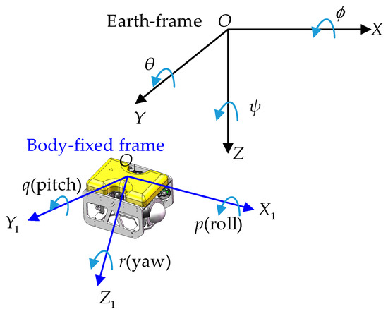
Figure 3.
Two coordinate systems for the AUV.
3.2. AUV Dynamic Model
The dynamic equation of the AUV’s motion can be given as follows [11,25,28]:
where is the inertial matrix, which includes the added mass; is the damping matrix; is the gravitational terms matrix; is the matrix of Coriolis and centripetal terms; is the position and orientation vector; is the control forces vector. The AUV’s gravitational and buoyancy centers are located at one point. The translational and rotational motions can be described with six equations, which denote surge, sway, heave, roll, pitch, and yaw, respectively as follows:
where m is the AUV’s mass; and are the location parameters of the AUV’s gravitational centers; , , are the AUV’s inertia mass moments; , , , , and are the speed coefficients; , , , , , , are the second-order speed coefficients; and are the second-order speed coefficients; and are the vertical angle and horizontal fins, respectively; is the propeller thrust; and is the propeller torque.
It should be noted that one can select several equations from Equations (11) to (16) for path-tracking design according to the actual engineering.
4. AUV Path Tracking with the Fuzzy Controller
4.1. The Design of the Fuzzy Controller
Fuzzy control is a human-like intelligent control method embodying the human control experience and strategy [29]. Fuzzy control does not depend on the precise models of the nonlinear control system, which can be used in the control process with strong robustness and good anti-interference performance [30,31,32]. A fuzzy controller contains four basic elements: fuzzification, knowledge base, fuzzy inference and defuzzification.
In this paper, we select triangle membership function for fuzzification, the reasons are given as follows: (1) Consisting of simple straight-line segments, triangular membership function is very easy to apply in fuzzy control; (2) Triangular membership function can obtain good performance for AUV control [30]. The methodologies to use for membership function optimization are given as follows: the membership function is assumed as an isosceles triangle, the function includes three parameters; the first and third parameters are optimized by the PSO algorithm, the middle is obtained as the average of the first and third values. Input parameters and are transformed into fuzzy information based on the given triangle membership function. Based on the results of different fuzzy control rules with a trial-and-error method, Table 1 can be obtained with the fuzzy control rules for AUV path tracking. Combined with the input parameters, the output parameters attitude angles are obtained according to the fuzzy control rules, which are changed with and . The center of gravity method has smooth output inference control, whose output changes in response to small changes in the input value. Therefore, we select the center of gravity method for defuzzification in this paper.

Table 1.
Fuzzy control rules for the AUV.
Remark 1.
NB denotes negative big, NM denotes negative middle, NS denotes negative small, ZO denotes zero, PS denotes positive small, PM denotes positive middle, PB denotes positive big.
In the control process for AUV path tracking, once the coordinates of the current and target locations are given, the desired attitude angles can be obtained at the desired AUV velocity [17]. Therefore, we select not only the cross-track position and attitude angle errors but also their derivatives as the input parameters. Figure 4 and Figure 5 show the membership functions of cross-track position errors and corresponding derivatives, respectively, which are like the ones for cross-track attitude angle errors and their derivatives. Input and output variables need to be divided into different fuzzy sets. The more numbers of the fuzzy sets, the more detailed and flexible for the constituted fuzzy control rules, this may increase the programming complexity and computing time. Conversely, the less numbers of the fuzzy sets, the less simple the fuzzy control rules, this may lead to difficulties for the controller to achieve the expected effect. We divide input and output variables into seven fuzzy sets based on the experiment, which are good enough to balance the calculation time and control accuracy. The fuzzy states of cross-track position errors and their derivatives are given as follows: (1) Cross-track position error () is divided into seven fuzzy states as follows, , , , , , , ; (2) Cross-track position error derivative is divided into seven fuzzy states as follows: , , , , , , . Similar to Figure 4 and Figure 5, the fuzzy states of the attitude angles and their derivatives can be given as follows: (1) Cross-track attitude angle error is divided into seven fuzzy states as follows: , , , , , , ; (2) Cross-track attitude angle error derivative is divided into seven fuzzy states as follows: , , , , , , .
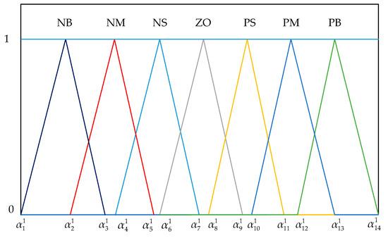
Figure 4.
Membership function of the cross-track position error.
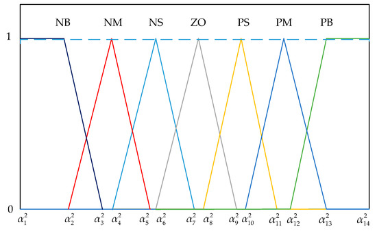
Figure 5.
Membership function of the corresponding derivative.
Remark 2.
Cross-track attitude angle errors include the cross-track roll, pitch, and yaw (heading) angle errors in the three-dimensional environment, cross-track attitude angle error is the heading angle error if just considering path tracking in the XOY plane, the definition is given in Section 2.
4.2. The Optimization for the Fuzzy Controller
In this paper, fuzzy control converts a linguistic control strategy into an automatic controller capable of managing the AUV path-tracking system. The membership function greatly affects the performance of the fuzzy controller, whose parameters are usually obtained by the cut-and-trial method with many experiments. This takes a lot of time and increases the difficulty to obtain the optimal value. Therefore, an algorithm needs to optimize the controller to ensure the control performance.
PSO is a popular and efficient method to solve many different kinds of engineering optimization problems [33,34]. The PSO algorithm has been proven to be simple for formulation, easy for programming and has good convergence [35,36,37,38], this conclusion is verified for fuzzy controller optimization of AUV path tracking. The PSO algorithm simulates the foraging behavior of a flock of flying birds, the result is achieved through cooperation and competition between individuals in the flock. In the PSO algorithm, flying “birds” are simulated by particles without weight or volume, each potential solution is represented by one particle in the search space, and its “flight state” is denoted with both the velocity and position of the particle. The global optimal search is realized by the particles, which continuously learns from the group and neighborhood optimal solutions. The new particle position and velocity can be obtained as follows [39,40]:
where is the current velocity of one particle; is the new velocity of one particle; is the iteration; is the inertia weight; is the social acceleration for the local best position; is the cognitive acceleration for the global best position; and are random numbers between 0 and 1; and are the best solutions found by a particle and in a population, respectively; is the current position; is the new position; is the maximum number of iterations; is the current number of iteration; and and are the initial and final inertia weight, respectively.
In this paper, the following function is given to optimize the fuzzy controller to improve the path-tracking performance.
where is the optimization performance index including , and ; is the length of the tracking path; is the smoothness of the tracking path; and is the average cross-track position error. To solve the multiple objective functions for path tracking, a weight coefficient method is presented to transform Equation (20) as follows:
where , , are the weight coefficients; and , , are the normalized values of , , respectively.
- (1)
- Tracking path length
The start and target points are and for the path, respectively, and is the total number of the segments of the tracking path. The path can be expressed as follows: .
The total length of the tracking path can be obtained as follows [22,41]:
where is one point of the tracking path at , and is the corresponding serial segment number. is the length from the adjacent point to , which can be calculated as follows:
- (2)
- Tracking path smoothness
A virtual triangle is used to describe the path smoothness, which is composed of three adjacent points , , and . The cosine function is given to obtain the intersection angle for the AUV tracking path as follows.
where is the intersection angle with the corner vertex of (). , , and are the lengths of triangle sides with the angles of , , and , respectively. is the intersection angle with the corner vertex of (); and is the intersection angle with the corner vertex of (). is the AUV tracking path smoothness, the smaller , the better the path smoothness. , is the serial number of the corner for each turning point.
- (3)
- Cross-track position error
The average of the total absolute of the cross-track position errors is given as a performance index, which is referred to simply as the average cross-track position error in this paper, calculated as follows:
where is the average of the total ; is one cross-track position error; and denotes the absolute value of .
Figure 6 shows the flowchart of the path tracking in light of the fuzzy controller with the PSO algorithm, algorithm 1 presents the path-tracking steps in detail.
| Algorithm 1: The path-tracking algorithm |
| 1: Establishing the AUV kinematic model (Equation (7)) and the dynamic model (Equation (10)), obtaining the optimization function (Equation (21)) for the fuzzy controller for path tracking; |
| 2: Defining the rules for the fuzzy controller, setting the basic initial parameters of the triangle membership function; |
| 3: Initializing the parameters including , , and so on; |
| 4: Setting the AUV start point as , ; |
| 5. Obtaining the target point of the desired path ; |
| 6: Calculating the errors and these derivatives of the input parameters of the fuzzy controller, executing fuzzification optimization; |
| 7: Realizing the fuzzy inference based on the membership functions, executing the defuzzification operation; |
| 8: Calculating the fitness functions of each particle based on Equation (21), obtaining the optimization particle position; |
| 9: Updating the current velocity of each particle based on Equations (17)–(19); |
| 10: If is smaller than , go to the next step, else if, obtain the parameters of membership functions, setting , go to step 7; |
| 11: Obtaining the tracking point based on the AUV kinematic and dynamic models, if is smaller than , setting , go to step 4, else if, go to the next step; |
| 12: Obtain the optimal tracking path. |
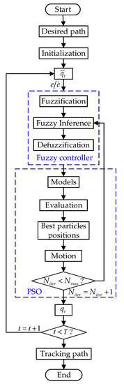
Figure 6.
Flowchart for path tracking with the fuzzy controller.
5. Results and Discussion
In this section, a self-made “Ocean Star” AUV is used to illustrate the effectiveness of the proposed algorithm. Figure 7 gives the “Ocean Star” AUV and its configuration, the length is 400 mm, the width is 295 mm, and the high is 255 mm. Six thrusters are given to provide forces to control the AUV, Figure 7b shows the corresponding configuration.
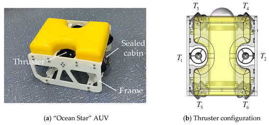
Figure 7.
The mechanical structure and physical drawing.
Different scenarios are given including straight line, sine, half-moon shape, Archimedean spiral, and practical paths tracking. For the PSO algorithm, the initial value of the inertia weight , the social and cognitive accelerations are and , respectively. In general, the fewer particles, the more iterations are required to obtain good optimization results. For example, the algorithm needs more than 100 iterations with 15 particles and 160 iterations with 10 particles to guarantee the optimization results. In this paper, the number of particles and the maximum number of iterations are good enough for the proposed algorithm with the settings as follows: the number of the particles is 20 for the group, the maximum number of iterations is 50. We set the weight coefficients as , , and for the optimization objective functions.
A desired straight line is given as follows: , , where (as shown in Figure 8). The straight line is discretized by the sequential discrete points , and the corresponding start point is . The initial position, Euler angle, and velocity are set to , , , respectively. The desired velocity is set to . Figure 8 shows the desired and tracking path curves, we can see that the tracking path coincides well with the desired path. The tracking path length is 141.46 , smoothness is 982.4, and average cross-track position error is 0.078 . Figure 9 shows the cross-track position error, Figure 10 shows the heading angle error. The cross-track position and heading angle errors become smaller and smaller over time. The cross-track position error is limited in the range of , and the standard deviation is 0.007 for path cross-track position errors calculated from the start to the target tracking points. The cross-track heading angle error is limited in the range of , and the standard deviation is 0.0045 for the cross-track heading angle errors calculated from the start to the target tacking points. The proposed fuzzy controller with the PSO algorithm can deal with straight line path tracking practically and effectively.
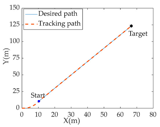
Figure 8.
Path tracking results for the straight line.
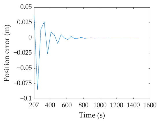
Figure 9.
Cross-track position error for the straight line.
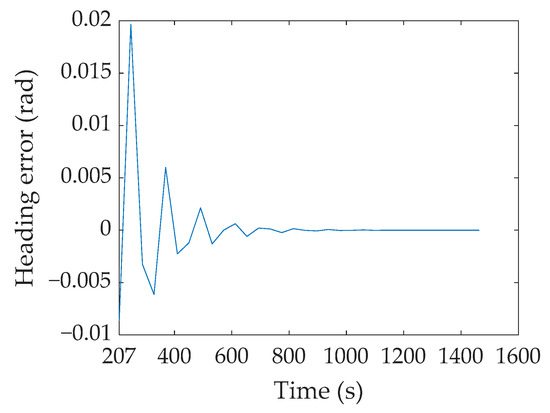
Figure 10.
Cross-track heading angle error for the straight line.
The desired sine curve path is given as follows: , , where , Figure 11 shows the corresponding curve. The sine curve is discretized by the sequential discrete points , and the corresponding start point is . The initial position, Euler angle, and velocity are set to , , and , respectively. The desired velocity is set to . Figure 11 shows the tracking path by the proposed algorithm, the tracking path length is 259.52 , smoothness is 1802.2, and average cross-track position error is 0.18 . Figure 12 shows the cross-track position error, Figure 13 shows the cross-track heading angle error. The cross-track position error is limited in the range of , and the standard deviation is 0.25 for the path-tracking position. The cross-track heading angle error is limited in the range of , and the standard deviation is 0.08 for the cross-track heading angle error. Although larger values are at the peaks and valleys of the cross-track position and heading angle errors, the tracking path still coincides well with the desired curve. The proposed fuzzy controller with the PSO algorithm can deal with sine curve path tracking practically and effectively.
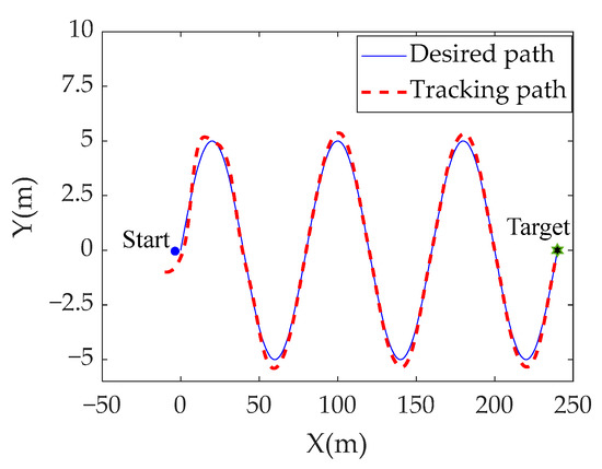
Figure 11.
Path-tracking results for the sine curve.
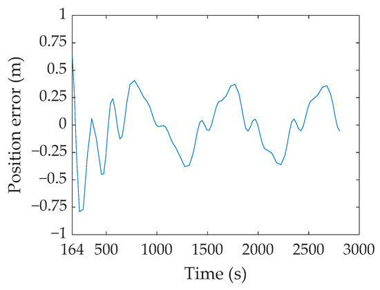
Figure 12.
Cross-track position error for the sine curve.
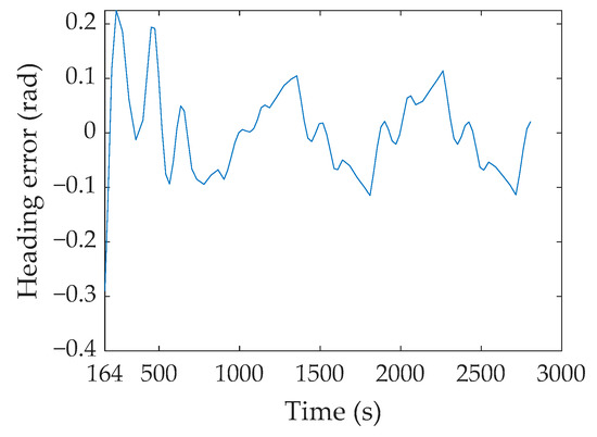
Figure 13.
Cross-track heading angle error for the sine curve.
The desired half-moon shape path is given as follows: , , where . , , where . Figure 14 shows the half-moon shape path, which is discretized by the sequential discrete points . The start and target points are all at for the desired path, the AUV moves along the half-moon shape in an anti-clockwise direction. The initial position, Euler angle, and velocity are set to , , and , respectively. The desired velocity is set to . Figure 14 shows the tracking path by the proposed algorithm, the red curve coincides well with the desired path. The tracking path length is 278.38 , smoothness is 1931.5, and average cross-track position error is 0.17 . Figure 15 and Figure 16 show the cross-track position and heading angle errors, respectively. The standard deviation is 0.38 for the path cross-track position calculated from the start to the target tracking points. The standard deviation is 0.11 for the cross-track heading angle error calculated from the start to the target tracking point. The proposed fuzzy controller algorithm can deal with the half-moon shape path tracking practically and effectively.
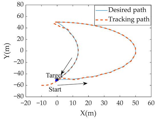
Figure 14.
Tracking results for the half-moon shape.
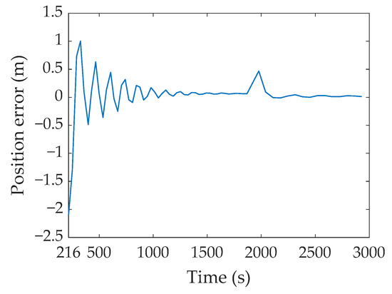
Figure 15.
Cross-track position error for the half-moon shape.
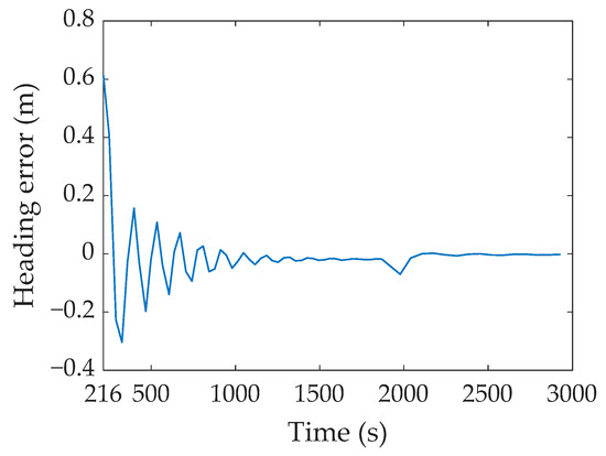
Figure 16.
Cross-track heading angle error for the half-moon shape path.
Some comparison results are given to make an in-depth analysis of the path-tracking simulation results. A desired Archimedean spiral path is given as follows: , , where . Figure 17a shows the Archimedean path, which is discretized by the sequential discrete points , the corresponding start point is . It should be noted that Figure 17b is a partial enlargement of Figure 17a. The initial position, Euler angle, and velocity are set to , , and , respectively. The desired velocity is set to . Figure 18 and Figure 19 show the comparison tracking results between the proposed algorithm, fuzzy control method (using only fuzzy logic), and the traditional method (PID algorithm). Table 2 gives the corresponding comparison with some performance indexes. The tracking path length is 360.9 , smoothness is 1353, and average cross-track position error is 0.05 by the proposed algorithm. The tracking path length is 361.2 , smoothness is 1355, and average cross-track position error is 0.06 by the fuzzy control method. The tracking path length is 361.8 , smoothness is 1357, and average cross-track position error is 0.09 by the traditional method. Figure 18 shows the cross-track position error for the Archimedean spiral. The fluctuating range of the error curve by the proposed algorithm is smaller than the fuzzy control and traditional methods. The standard deviations of the cross-track position errors are 0.065 , 0.078 , and 0.113 by the proposed, fuzzy control, and traditional methods, respectively. The proposed algorithm obtains better tracking results compared with the fuzzy control and traditional methods.
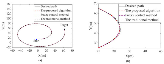
Figure 17.
(a). Path-tracking results for Archimedean spiral. (b) Partial enlargement for the tracking path.
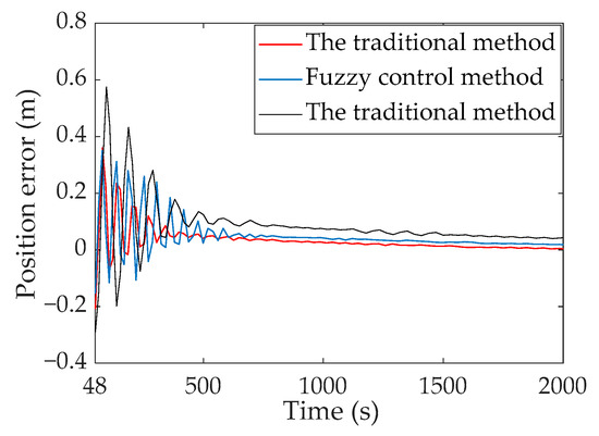
Figure 18.
Cross-track position error for the Archimedean spiral.
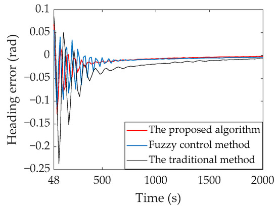
Figure 19.
Cross-track heading angle error for the Archimedean spiral.
Table 2.
Comparison of the proposed and existing algorithms.
Figure 20 and Figure 21 show a desired path in the real environment of our university. The length and width are obtained for a man-made river with an irregular polygon shape based on a diastimeter. The desired path is the line with a distance of 1 from the riverbank to the AUV’s center. As shown in Figure 21, we establish the coordinate system (XOY), and select a point of the bottom left corner of the river as the origin. The AUV start and target positions are at the same point , and the AUV moves along the path in a clockwise direction. The initial Euler angle is , the initial velocity is , and the desired velocity is . Figure 21 shows the tracking results, the tracking path length is 99.14 , smoothness is 633.59, and average cross-track position error is 0.05 . Figure 22 shows the cross-track position error, and the standard deviation is 0.1 of the cross-track position errors. Figure 23 shows the cross-track heading angle error, and the standard deviation is 0.04 of the cross-track heading angle errors. Results show that the AUV can follow the path effectively by the proposed algorithm.
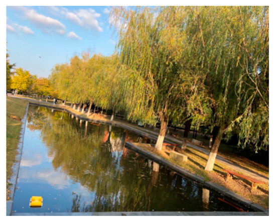
Figure 20.
The desired path in a real man-made river.
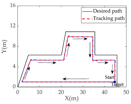
Figure 21.
The path tracking in the real man-made river.
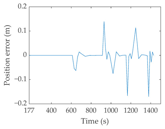
Figure 22.
Cross-track position error for the AUV.
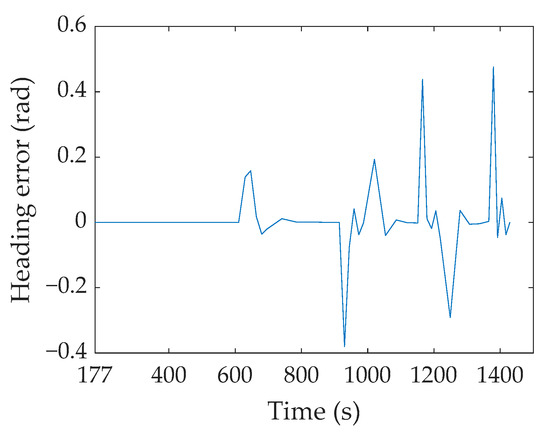
Figure 23.
Cross-track heading angle error for the AUV.
6. Conclusions
AUV path tracking is important to realize for AUV application in numerous missions for the exploration of marine resources. In this paper, a fuzzy controller was designed with multiple performance optimizations to complete path tracking. Based on the established AUV kinematic and dynamic models, we selected the path length, smoothness and cross-track position error as the objective functions of the optimization problem for the fuzzy controller. The PSO algorithm was used to optimize the membership function. We gave the straight line, sine curve, half-moon shape, Archimedean spiral, and practical paths to test the fuzzy controller’s performance for path tracking. The test results showed that the AUV effectively tracked the desired path using the proposed algorithm. Compared to the traditional algorithm, the designed controller made the path-tracking system perform well with better tracking accuracy, better smoothness and a shorter length using the proposed algorithm.
In the near future, we are interested in improving the path-tracking performance by incorporating salient features such as sliding mode control, deep reinforcement learning, and so on. Collaborative work on multiple AUVs is an important way to efficiently accomplish these missions, of which the key factor is how to accurately track multiple paths. Therefore, providing a method for multiple AUV path tracking is also our next work.
Author Contributions
Conceptualization, Q.T. and T.W.; methodology, Q.T.; software, T.W.; validation, Q.T., Y.W., Y.S. and B.L.; formal analysis, Q.T.; investigation, Q.T. and T.W.; resources, Y.W.; data curation, Y.S.; writing—original draft preparation, Q.T.; writing—review and editing, Y.W.; visualization, Y.S.; supervision, B.L.; project administration, B.L.; funding acquisition, Y.W. All authors have read and agreed to the published version of the manuscript.
Funding
This research was funded by the China Post-doctoral Science Foundation (2022M710934), Post-doctoral Applied Research Project of Qingdao City, and the Project of Shandong Province Higher Educational Young Innovative Talent Introduction and Cultivation Team (Intelligent Transportation Team of Offshore Products).
Institutional Review Board Statement
Not applicable.
Informed Consent Statement
Not applicable.
Data Availability Statement
Not applicable.
Conflicts of Interest
The authors declare no conflict of interest.
References
- Hien, N.V.; Truong, V.-T.; Bui, N.-T.; de Oña, R. A Model-Driven Realization of AUV Controllers Based on the MDA/MBSE Approach. J. Adv. Transp. 2020, 2020, 8848776. [Google Scholar] [CrossRef]
- Marvian Mashhad, A.; Mousavi Mashhadi, S.K.-e.-d. PD like fuzzy logic control of an autonomous underwater vehicle with the purpose of energy saving using H∞ robust filter and its optimized covariance matrices. J. Mar. Sci. Technol. 2018, 23, 937–949. [Google Scholar] [CrossRef]
- Tian, Q.; Wang, T.; Liu, B.; Ran, G. Thruster Fault Diagnostics and Fault Tolerant Control for Autonomous Underwater Vehicle with Ocean Currents. Machines 2022, 10, 582. [Google Scholar] [CrossRef]
- Tran, H.N.; Nhut Pham, T.N.; Choi, S.H. Robust depth control of a hybrid autonomous underwater vehicle with propeller torque’s effect and model uncertainty. Ocean Eng. 2021, 220, 108257. [Google Scholar] [CrossRef]
- Bejarbaneh, E.Y.; Masoumnezhad, M.; Armaghani, D.J.; Pham, B.T. Design of robust control based on linear matrix inequality and a novel hybrid PSO search technique for autonomous underwater vehicle. Appl. Ocean Res. 2020, 101, 102231. [Google Scholar] [CrossRef]
- Yao, X.; Wang, X. Integral vector field control for three-dimensional path following of autonomous underwater vehicle. J. Mar. Sci. Technol. 2020, 26, 159–173. [Google Scholar] [CrossRef]
- Yang, X.; Yan, J.; Hua, C.; Guan, X. Trajectory Tracking Control of Autonomous Underwater Vehicle With Unknown Parameters and External Disturbances. IEEE Trans. Syst. Man Cybern. Syst. 2021, 51, 1054–1063. [Google Scholar] [CrossRef]
- Yu, C.Y.; Xiang, X.B.; Zuo, M.J.; Liu, H. Underwater cable tracking control of under-actuated AUV. In Proceedings of the 2016 IEEE/OES Autonomous Underwater Vehicles, Tokyo, Japan, 6–9 November 2016; IEEE: Piscataway, NJ, USA, 2016; pp. 324–329. [Google Scholar]
- Liu, F.; Shen, Y.; He, B.; Wang, D.; Wan, J.; Sha, Q.; Qin, P. Drift angle compensation-based adaptive line-of-sight path following for autonomous underwater vehicle. Appl. Ocean Res. 2019, 93, 101943. [Google Scholar] [CrossRef]
- Nie, W.; Feng, S. Planar path-following tracking control for an autonomous underwater vehicle in the horizontal plane. Optik 2016, 127, 11607–11616. [Google Scholar] [CrossRef]
- Zhang, G.; Huang, H.; Qin, H.; Wan, L.; Li, Y.; Cao, J.; Su, Y. A novel adaptive second order sliding mode path following control for a portable AUV. Ocean Eng. 2018, 151, 82–92. [Google Scholar] [CrossRef]
- Jia, C.; Chen, Z.; Zhang, G.; Shi, L.; Sun, Y.; Pang, S. AUV Tunnel Tracking Method Based on Adaptive Model Predictive Control. IOP Conf. Ser. Mater. Sci. Eng. 2018, 428, 012070. [Google Scholar] [CrossRef]
- Wang, D.; He, B.; Shen, Y.; Li, G.; Chen, G. A Modified ALOS Method of Path Tracking for AUVs with Reinforcement Learning Accelerated by Dynamic Data-Driven AUV Model. J. Intell. Robot. Syst. 2022, 49, 104. [Google Scholar] [CrossRef]
- Sun, Y.; Zhang, C.; Zhang, G.; Xu, H.; Ran, X. Three-Dimensional Path Tracking Control of Autonomous Underwater Vehicle Based on Deep Reinforcement Learning. J. Mar. Sci. Eng. 2019, 7, 443. [Google Scholar] [CrossRef]
- Yu, C.; Xiang, X.; Lapierre, L.; Zhang, Q. Nonlinear guidance and fuzzy control for three-dimensional path following of an underactuated autonomous underwater vehicle. Ocean Eng. 2017, 146, 457–467. [Google Scholar] [CrossRef]
- Zhang, J.; Xiang, X.; Lapierre, L.; Zhang, Q.; Li, W. Approach-angle-based three-dimensional indirect adaptive fuzzy path following of under-actuated AUV with input saturation. Appl. Ocean Res. 2021, 107, 102486. [Google Scholar] [CrossRef]
- Chen, J.; Zhu, H.; Zhang, L.; Sun, Y. Research on fuzzy control of path tracking for underwater vehicle based on genetic algorithm optimization. Ocean Eng. 2018, 156, 217–223. [Google Scholar] [CrossRef]
- Lee, H.J.; Rhee, K.P. Development of collision avoidance system by using expert system and search algorithm. Int. Shipbuild. Prog. 2001, 48, 197–212. [Google Scholar]
- Zhao, Y.; Li, W.; Shi, P. A real-time collision avoidance learning system for Unmanned Surface Vessels. Neurocomputing 2016, 182, 255–266. [Google Scholar] [CrossRef]
- Namgung, H.; Kim, J.S. Collision risk inference system for maritime autonomous surface ships using COLREGs rules compliant collision avoidance. IEEE Access 2021, 9, 7823–7835. [Google Scholar] [CrossRef]
- Namgung, H. Local route planning for collision avoidance of maritime autonomous surface ships in compliance with COLREGs rules. Sustainability 2021, 14, 198. [Google Scholar] [CrossRef]
- Ataei, M.; Yousefi-Koma, A. Three-dimensional optimal path planning for waypoint guidance of an autonomous underwater vehicle. Robot. Auton. Syst. 2015, 67, 23–32. [Google Scholar] [CrossRef]
- Wang, L.; Liu, L.; Qi, J.; Peng, W. Improved Quantum Particle Swarm Optimization Algorithm for Offline Path Planning in AUVs. IEEE Access 2020, 8, 143397–143411. [Google Scholar] [CrossRef]
- Cao, X.; Sun, H.; Jan, G.E. Multi-AUV cooperative target search and tracking in unknown underwater environment. Ocean Eng. 2018, 150, 1–11. [Google Scholar] [CrossRef]
- Taheri, E.; Ferdowsi, M.H.; Danesh, M. Closed-loop randomized kinodynamic path planning for an autonomous underwater vehicle. Appl. Ocean Res. 2019, 83, 48–64. [Google Scholar] [CrossRef]
- MahmoudZadeh, S.; Yazdani, A.M.; Sammut, K.; Powers, D.M.W. Online path planning for AUV rendezvous in dynamic cluttered undersea environment using evolutionary algorithms. Appl. Soft Comput. 2018, 70, 929–945. [Google Scholar] [CrossRef]
- Tian, Q.; Wang, T.; Wang, Y.; Li, C.; Liu, B. Robust Optimization Design for Path Planning of Bionic Robotic Fish in the Presence of Ocean Currents. J. Mar. Sci. Eng. 2022, 10, 1109. [Google Scholar] [CrossRef]
- Karkoub, M.; Wu, H.; Hwang, C. Nonlinear trajectory-tracking control of an autonomous underwater vehicle. Ocean Eng. 2017, 145, 188–198. [Google Scholar] [CrossRef]
- Ran, G.; Chen, H.; Li, C.; Ma, G.; Jiang, B. A Hybrid Design of Fault Detection for Nonlinear Systems Based on Dynamic Optimization. IEEE Trans. Neural Netw. Learn. Syst. 2022, 18, 1–11. [Google Scholar] [CrossRef]
- Xiang, X.; Yu, C.; Lapierre, L.; Zhang, J.; Zhang, Q. Survey on Fuzzy-Logic-Based Guidance and Control of Marine Surface Vehicles and Underwater Vehicles. Int. J. Fuzzy Syst. 2017, 20, 572–586. [Google Scholar] [CrossRef]
- Ran, G.; Liu, J.; Li, C.; Lam, H.; Li, D.; Chen, H. Fuzzy-Model-Based Asynchronous Fault Detection for Markov Jump Systems with Partially Unknown Transition Probabilities: An Adaptive Event-Triggered Approach. IEEE Trans. Fuzzy Syst. 2022, 11, 4679–4689. [Google Scholar] [CrossRef]
- Ran, G.; Shu, Z.; Lam, H.; Liu, J.; Li, C. Dissipative Tracking Control of Nonlinear Markov Jump Systems With Incomplete Transition Probabilities: A Multiple-Event-Triggered Approach. IEEE Trans. Fuzzy Syst. 2022, 20, 1–11. [Google Scholar] [CrossRef]
- Bangyal, W.; Hameed, A.; Alosaimi, W.; Alyami, H. A New Initialization Approach in Particle Swarm Optimization for Global Optimization Problems. Comput. Intell. Neurosci. 2021, 2021, 1–17. [Google Scholar] [CrossRef]
- Bai, B.; Guo, Z.; Zhou, C.; Zhang, W.; Zhang, J. Application of adaptive reliability importance sampling-based extended domain PSO on single mode failure in reliability engineering. Inf. Sci. 2021, 546, 42–59. [Google Scholar] [CrossRef]
- Bonyadi, M.R.; Michalewicz, Z. Particle swarm optimization for single objective continuous space problems: A review. Evol. Comput. 2017, 25, 1–54. [Google Scholar] [CrossRef] [PubMed]
- Yarat, S.; Senan, S.; Orman, Z. A Comparative Study on PSO with Other Metaheuristic Methods. Appl. Part. Swarm Optim.: New Solut. Cases Optim. Portf. 2021, 83, 49–72. [Google Scholar]
- Askarzadeh, A. Comparison of particle swarm optimization and other metaheuristics on electricity demand estimation: A case study of Iran. Energy 2014, 72, 484–491. [Google Scholar] [CrossRef]
- Ren, M.; Huang, X.; Zhu, X.; Shao, L. Optimized PSO algorithm based on the simplicial algorithm of fixed point theory. Appl. Intell. 2020, 50, 2009–2024. [Google Scholar] [CrossRef]
- Fattahi, P.; Hajipour, V.; Nobari, A. A bi-objective continuous review inventory control model: Pareto-based meta-heuristic algorithms. Appl. Soft Comput. 2015, 32, 211–223. [Google Scholar] [CrossRef]
- Pluhacek, M.; Senkerik, R.; Davendra, D.; Kominkova Oplatkova, Z.; Zelinka, I. On the behavior and performance of chaos driven PSO algorithm with inertia weight. Comput. Math. Appl. 2013, 66, 122–1234. [Google Scholar] [CrossRef]
- Tian, Q.; Wang, T.; Wang, Y.; Wang, Z.; Liu, C. A two-level optimization algorithm for path planning of bionic robotic fish in the three-dimensional environment with ocean currents and moving obstacles. Ocean. Eng. 2022, 266, 112829. [Google Scholar] [CrossRef]


Disclaimer/Publisher’s Note: The statements, opinions and data contained in all publications are solely those of the individual author(s) and contributor(s) and not of MDPI and/or the editor(s). MDPI and/or the editor(s) disclaim responsibility for any injury to people or property resulting from any ideas, methods, instructions or products referred to in the content. |
© 2023 by the authors. Licensee MDPI, Basel, Switzerland. This article is an open access article distributed under the terms and conditions of the Creative Commons Attribution (CC BY) license (https://creativecommons.org/licenses/by/4.0/).