Modeling and Adaptive Boundary Robust Control of Active Heave Compensation Systems

Abstract

Heave compensation systems are essential for operations’ safety, reliability, and efficiency in harsh offshore environments. This paper investigates the vibration suppression problem of a type of deep-sea robot with the length of time variation and harsh operating environments for active heave compensation systems, where hydraulic heave compensators implement actuators with input nonlinearity, model coupling, and unknown nonlinear disturbances. A robust adaptive output feedback control scheme based on the backstepping control method is designed to eliminate deep-ocean robot vibration, where the adaptive law handles the system parameter uncertainty. Meanwhile, a nonlinear disturbance observer (NDO) is introduced to overcome the effects of random disturbances and model coupling. In addition, the stability of the whole system is proved according to Lyapunov’s theory, and the scheme is shown to be feasible by theoretical analysis. Finally, a comparative simulation study was conducted to validate the effectiveness of the proposed controller.

1. Introduction

With the rapid growth of modern industry, the development of marine resources has been promoted. Still, it is a challenging task to move equipment and operations on rough seas [1]. This challenge has stimulated and driven the rapid development of remotely operated vehicle (ROV) technology [2]. Underwater robots are essential pieces of technology for marine exploration and the exploitation of deep-sea resources. They allow operators to remotely control the robots from surface vessels, making them indispensable tools for deep-sea operations. Due to their remarkable features, such as high efficiency, cost-effectiveness, large operating depth, and safety, underwater robots have become a high-tech means of conducting deep-sea missions [3].

However, the marine environment is complex and volatile. The ship is subject to significant free motion in extreme sea conditions, which includes mainly heaving, flat rocking, transverse rocking, and longitudinal rocking motion, which will lead to dramatic changes in the heaving motion amplitude and umbilical cable tension of the underwater robot, seriously affecting the safety and efficiency of marine operations [4]. To address the previous questions, heave compensation systems have been researched and developed in the past few decades and are widely used in marine operation equipment such as for deep-sea exploration, deep-sea salvage, and deep-sea oil and gas extraction [5]. Furthermore, they can eliminate the lifting and sinking motion of the surface vessel relative to the underwater robot, thus avoiding the impact load caused by the cable’s slack and effectively preventing the damage and breakage of the cable [6]. The active heave compensation system consists of sensors that detect the current motion state of the vessel and the underwater robot and transmit it to the controller, which then actively compensates for it via a flexible umbilical cable. The hydraulic unit supplies power to the controller, as shown in Figure 1, which regulates the vertical umbilical cable length utilizing a hydraulic cylinder. Since the system is a distributed parameter system, and the robot heave compensation is performed by a single control input at the hydraulic cylinder, more complex nonlinear dynamic characteristics must be considered in the feedback control design [7].

Figure 1. Active heave compensation for ROV.

The primary function of the heave compensation system is to reduce underwater robot vibration and prevent tension slack in the umbilical cable during offshore operations. Woodacre et al. demonstrated the development and results of a model-predictive controller (MPC) for a marine active heave compensation (AHC) system (a type of control system used in offshore operations, particularly in the oil and gas industry) [8]. It is designed to stabilize the motion of a vessel, such as a drilling rig or a floating production platform, by compensating for the vertical movement caused by waves and currents. In this reference, a control algorithm of the proposed hydraulic active heave compensation system is developed using singular perturbation theory to cancel the relative motion between the spar top and gripped preassembly bottom [9]. Under various factors, Liu et al. investigated the dynamics of longitudinal and transverse coupling vibration of suspended riser pipes on deep-sea drilling platforms. They showed that the longitudinal vibration of riser pipes was mainly caused by vessels’ lifting and sinking motion on the sea surface [10]. Lee et al. investigated the dynamic characteristics of cables. They introduced control methods such as PID, sliding mode, and linear feedback to suppress overhead crane vibrations and reduce heaving movements [11]. However, in the deep-ocean robot lifting system, the umbilical cable and the underwater robot are frequently interfered with by different nonlinear elements, including the nonlinear disturbance forces generated by undulating wave movement and the nonlinear dynamics and uncertainties of hydraulic systems, which are insufficient to be satisfied by the traditional control strategy [12]. Therefore, the online estimation and adjustment of design parameters in active heave compensation systems can be a practical approach for improving control performance [13]. Cao et al. applied adaptive control techniques for a class of semi-strict feedback systems, which can achieve high tracking accuracy for nonlinear systems even when the control parameters are unknown [14]. Nevertheless, conventional adaptive control is susceptible to random interference and degraded control performance.

Robust control is particularly suitable for systems with unknown bounded perturbations. It has been widely used to overcome engineering challenges [15] such as motor control, robot control, etc. Xing et al. designed a robust adaptive control for a flexible manipulator system with uncertain disturbance effects, and the controller effectively suppressed the flexible manipulator’s deformation [16]. Facing the uncertainty of the system, Islam et al. investigated robust sliding mode control to achieve the accurate tracking of the flexible manipulator, which significantly reduces the impacts of unknown disturbances [17]. Li et al. proposed an ADRC-ESMPC dual-loop controller to be used in an active lift–sink compensation system based on a hydraulic valve, and the simulation demonstrated the validity of the controller [18]. Yu et al. applied state-constrained variable structure control to an active heave compensation system and verified the effectiveness of the controller through experiments [19].

On the other hand, disturbance observer-based control techniques have progressed over the past decades. They handle uncertainties in the model and compensate them feed-forwardly [20,21,22]. Sun et al. proposed an observer-based state feedback control scheme to reduce the vibration of flexible cables without measuring the velocity signal of the feedback control, and the results showed that the method is more efficacious [23]. The strict form of feedback is achieved by backstepping, but the iterative computation of backstepping leads to a “complexity explosion” [24]. To avoid the repeated differentiation of higher-order terms, Kim et al. used a dynamic surface control method to make the design of the controller facile by introducing a first-order filter to change the differentiation operation into a simple algebraic process [25]. Shi et al. combined a BP neural network and a PID controller and applied them to the active–passive integrated heave compensation model, and the hook displacement compensation rate of the crane device could reach more than 90% [26]. However, most heave compensation studies have focused only on fixed-length umbilical cables and ignored time-varying-length umbilical cables. Currently, during the lowering and retrieval phases of the robot, it is equally threatened by waves that cause the slack or breakage of the cable. Therefore, there is an urgent need for an active heave displacement compensation method that can be applied to time-varying-length umbilical cable lifting systems. To overcome the above difficulties, this article establishes a theoretical model of an active heave compensation system for deep-ocean robots and designs a controller based on the model to realize the displacement compensation of deep-sea robots under unknown external perturbations and internal coupling.

The other parts of the paper are arranged as follows. Section 2, a mathematical model of the active heave compensation system for deep-sea robots, is established based on Hamilton’s principle. The nonlinear disturbance observer (NDO) and the robust adaptive feedback control are designed according to the backstepping control in the following section. Section 4 carries out a comparison of the simulation results to prove the effectiveness of the proposed control method. Finally, some conclusions are presented.

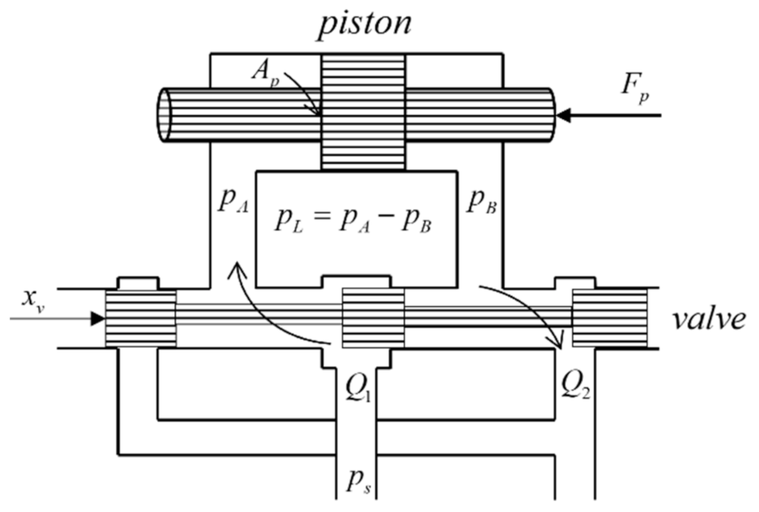
2. Dynamic Modeling

Vibration Control Equations

Considering the working principle of the active heave compensation system, the umbilical cable lifting system is represented by a typical distributed parameter model. Among them, the critical variables in the model are listed Table 1. And some other symbols are shown as Appendix A (Table A1).

Table 1. System parameter nomenclature.

Symbol	Definition	Symbol	Definition
$m_p$	Quality of the robot	$m_t$	Quality of the piston
$u\left(x,t\right)$	Vibration of cable at x	$x_p$	Piston displacement
$u_t\left(x,t\right)$	Partial differentiation with t	$\rho$	Hydraulic oil density
$u_x\left(x,t\right)$	Partial differentiation with x	$A_p$	Active area
$l\left(t\right)$	Time-varying length	$x_v$	Valve spool displacement
${\rho }_l$	Linear density	$K_q$	Flow Gain
$c$	Viscous damping	$K_c$	Flow-pressure coefficient
${\beta }_e$	Hydraulic oil bulk modulus of elasticity	$C_d$	Flow coefficient
$p_s$	Supply pressure	$w_v$	Throttle window area gradient
$B_p$	Damping coefficient	$C_{tp}$	Total leakage coefficient

In this paper, the ROV lowering direction is chosen as the coordinate positive direction, and then the varying length of the vertical cable during the ROV lowering and raising can be represented as $l\left(t\right)$, and then the running speed and acceleration are, respectively, expressed as $v\left(t\right)=\dot{l}\left(t\right)$ and $a\left(t\right)=\ddot{l}\left(t\right)$. Neglecting the lateral vibration of the ROV, the longitudinal vibration displacement of the vertical section of the umbilical cable is defined as $u\left(x,t\right)$, and the introduction of differential operators “ D/Dt” is expressed as

$$\frac{D}{Dt}=\frac{\partial }{\partial t}+v\left(t\right)\frac{\partial }{\partial x}$$

(1)

The kinetic energy of the ROV active lifting and sinking compensation system is mainly composed of the kinetic energy of the umbilical cable, the hydraulic cylinder piston, and the kinetic energy of the ROV.

The potential energy in the system is composed of two main parts; one is the elastic potential energy of the umbilical cable, and the other is the gravitational potential energy of the ROV and the umbilical cable. The entire potential energy and the total virtual work are obtained as follows

$$E_k=\frac{1}{2}{\rho }_l{\displaystyle {\int }_0^l{\left(\frac{Du\left(x,t\right)}{Dt}+v\right)}^{2}dx}+\frac{1}{2}{m}_t{u}_t{\left(0,t\right)}^2+\frac{1}{2}{m}_p{\left(\frac{Du\left(l,t\right)}{Dt}+v\right)}^2$$

(2)

$$E_p=\frac{1}{2}EA{\displaystyle {\int }_0^l{u}_x^2\left(x,t\right)}dx-{\displaystyle {\int }_0^l{\rho }_{l}gu\left(x,t\right)dx-m_{p}gu\left(l,t\right)}$$

(3)

$$W=\left(F_l+d_t\left(t\right)\right)u\left(0,t\right)+d_p\left(t\right)u\left(l,t\right)-B_p{u}_t\left(0,t\right)-C\frac{Du\left(l,t\right)}{Dt}-c{\displaystyle {\int }_0^l\frac{Du\left(x,t\right)}{Dt}dx}$$

(4)

where $EA$ is the axial tensile stiffness of the umbilical cable, and the symbol g is the acceleration of gravity. $F_l$ is expressed as hydraulic compensation system external load force, $d_t\left(t\right)$ is expressed as an unknown disturbance to the hydraulic system, and $d_p\left(t\right)$ is expressed as the boundary disturbance force on the ROV. $B_p$ is defined as the hydraulic cylinder piston damping coefficient. $C$ indicates the ROV underwater damping coefficient, and $c$ represents the damping coefficient of the vertical section of the umbilical cable. Therefore, the kinetic equation can be reduced to a partial differential equation and two boundary conditions

$$\begin{array}{l}{\rho }_l\left(\frac{D^{2}u\left(x,t\right)}{D{t}^2}+a\right)+c\frac{Du\left(x,t\right)}{Dt}-EA{u}_{xx}\left(x,t\right)={\rho }_{l}g,\forall x\in \left(0,l\right)\times \left[0,\infty \right)\\ m_t{u}_{tt}\left(0,t\right)+B_p{u}_t\left(0,t\right)-EA{u}_x\left(0,t\right)=F_l+d_t\left(t\right),x=0\\ m_p\left(\frac{D^{2}u\left(l,t\right)}{D{t}^2}+a\right)+C\frac{Du\left(l,t\right)}{Dt}+EA{u}_x\left(l,t\right)=m_{p}g+d_p\left(t\right),x=l\end{array}$$

(5)

where $\frac{D^{2}u\left(x,t\right)}{D{t}^2}=u_{tt}+2v{u}_{xt}+a{u}_x\left(x,t\right)+v^2{u}_{xx}$.

Since Equation (5) is a partial differential equation with infinite degrees of freedom and many parameters are time-varying, it is complicated to solve it directly. Therefore, the infinite partial differential equations are generally transformed into finite-dimensional ordinary differential equations using the newly modified assumption modal method for this class of partial differential equations. Then, the ordinary differential equations are solved by numerical methods.

Therefore, a new variable $\xi$ is defined to normalize the original variable $x$ for the transformation of the time-varying domaininto a fixed domain $\left[0,1\right]$ of $\xi$, where $\xi =x/l\left(t\right)$. Assume that the solution of the system can be approximated by a limited number of linear compositions of known modal functions $\widehat{u}\left(\xi ,t\right)$

$$\widehat{u}\left(\xi ,t\right)=F_0\left(\xi \right)u\left(0,t\right)+F_1\left(\xi \right)u\left(l,t\right)+{\displaystyle \sum _{i=1}^n{\psi }_i\left(\xi \right)}{q}_i\left(t\right)$$

(6)

where $F_0\left(\xi \right)u\left(0,t\right)+F_1\left(\xi \right)u\left(l,t\right)$ is used to approximate the boundary condition term, and ${\displaystyle \sum _{i=1}^n{\psi }_i\left(\xi \right)}{q}_i\left(t\right)$ to approximate internal longitudinal vibration. ${\psi }_i\left(\xi \right)$ and $q_i\left(t\right)$ denote the trial function and the time-dependent generalized coordinate vector only, respectively, which can be expressed as $\psi \left(\xi \right)={[{\psi }_1(\xi ),{\psi }_1(\xi ),\dots ,{\psi }_n(\xi )]}^T$, $q\left(t\right)={[q_1(t),q_2(t),\dots ,q_n(t)]}^T$, where the variable n is the positive integer. To satisfy the geometric boundary conditions, $F_0\left(\xi \right)$ and $F_1\left(\xi \right)$ are chosen as $F_0\left(\xi \right)=1-\xi$, $F_1\left(\xi \right)=\xi$, ${\psi }_i\left(\xi \right)=\sqrt{2}\sin \left(i\pi \xi \right)$, $i=1~n$.

Before solving for the ROV active heave compensation system, an approximate solution of the equation is first expanded by the partial derivatives in the equation, using $\xi$ and $t$ as independent variables. Combining Equation (6) with $Du\left(l,t\right)/Dt$, we obtain

$$\frac{D^{2}u\left(l,t\right)}{D{t}^2}={\left.\left({\widehat{u}}_{tt}+\frac{2v}{l}\left(1-\xi \right){\widehat{u}}_{\xi t}+\frac{v^2}{l^2}{\left(1-\xi \right)}^2{\widehat{u}}_{\xi \xi }+\frac{al-2v^2}{l^2}\left(1-\xi \right){\widehat{u}}_{\xi }\right)\right|}_{\xi =1}={\widehat{u}}_{tt}\left(1,t\right)$$

(7)

Substituting Equations (6) and (7) into Equation (5), update the boundary condition equations

$$\begin{array}{l}m\ddot{u}\left(0,t\right)+B_p\dot{u}\left(0,t\right)-K\left[u\left(1,t\right)-u\left(0,t\right)\right]=U\left(t\right)+F_l+d_2\left(t\right),\xi =0\\ M\ddot{u}\left(1,t\right)+C\dot{u}\left(1,t\right)+K\left[u\left(1,t\right)-u\left(0,t\right)\right]=m_p\left(g-a\right)+d_1\left(t\right),\xi =1\end{array}$$

(8)

where $M$ and $m$ are expressed as $M=\left(m_p+{\rho }_{l}l{\displaystyle {\int }_0^1{F}_1\left(\xi \right)}d\xi \right)$ and $m=\left(m_t+{\rho }_{l}l{\displaystyle {\int }_0^1{F}_0\left(\xi \right)}d\xi \right)$, respectively. $K$ is the time-varying stiffness of the umbilical cable, expressed as $K=EA/l\left(t\right)$. $d_1$ and $d_2$ are uncertainty terms, $d_1\left(t\right)=-K{\displaystyle \sum _{i=1}^n{\psi }_i^T\left(1\right)q_i\left(t\right)}+d_p\left(t\right)$, $d_2\left(t\right)=K{\displaystyle \sum _{i=1}^n{\psi }_i^T\left(0\right)q_i\left(t\right)}+d_t\left(t\right)$.

To facilitate the design of the hydraulic compensation system, it is necessary to simplify the system, and several assumptions can be made:

• Ignoring the effect of system piping pressure loss and dynamic properties;
• Neglecting servo valve flow leakage;
• The system supply pressure is stable and unchanging and oil tank pressure is 0.

Figure 2 shows the principal graph of the hydraulic compensation system. The compensation system is mainly made up of hydraulic cylinders and servo valves, as the servo valve often moves near the steady-state operating point, so the servo valve spool moves to the right as the positive direction. The servo valve flow equation can be expressed as

$$Q_L=K_q{x}_v-K_c{p}_L$$

(9)

where $x_v$ is the servo valve spool displacement, $K_q$ is the servo valve flow gain, and $K_c$ is the servo valve flow-pressure coefficient.

$$K_q=C_d{w}_v\sqrt{\frac{1}{\rho }\left[p_s-\mathrm{sgn}\left(x_v\right)p_L\right]}$$

(10)

$$K_c=-\frac{C_d{w}_v\left|x_v\right|\sqrt{\frac{1}{\rho }\left(p_s-\mathrm{sgn}\left(x_v\right)p_L\right)}}{2\left(p_s-p_L\right)}$$

(11)

$p_L$ is the hydraulic cylinder load pressure drop, which can be expressed as $p_L=p_A-p_B$, where $C_d$ is the servo valve flow coefficient, $w_v$ is the servo valve throttle window area gradient, $\rho$ is the hydraulic fluid density, and $p_s$ is the oil supply pressure. The symbol $sgn\left(·\right)$ is a signed function.

Figure 2. Hydraulic compensation system.

Since the dynamic response speed of the hydraulic cylinder is much smaller than the dynamic response speed of the servo valve, omitting the servo valve dynamics model does not decrease the precision of the system, so the dependency between the spool displacement and the control input voltage can be written as $x_v=k_v{u}_v$, where $k_v$ indicates the servo valve control voltage-spool displacement conversion coefficient, and $u_v$ expresses the servo valve control current. Therefore, the servo valve flow equation is further written as $Q_L=K_q{k}_v{u}_v-K_c{p}_L$. When a hydraulic piston is in the neutral position of the cylinder at the initial moment and performs a small amplitude displacement, and in the course of work to satisfy $p_s=p_A+p_B$, the hydraulic cylinder flow continuous formula can be written as

$$Q_L=A_p\frac{d{x}_p}{dt}+C_{tp}{p}_L+\frac{V_t}{4{\beta }_e}\cdot \frac{d{p}_L}{dt}$$

(12)

where $A_p$ indicates the effective piston area, $C_{tp}$ expresses the total system leakage coefficient, $V_t$ indicates the total effective volume of the cylinder, and ${\beta }_e$ is the bulk modulus of elasticity of hydraulic fluid. $x_p$ indicates piston displacement, and $x_p=u\left(0,t\right)$.

The hydraulic cylinder used in the compensation system is a servo cylinder, and compared with the external load, the Coulomb friction between the piston and cylinder barrel of the hydraulic cylinder is negligible; therefore, based on Newton’s second law, the load force balance equation for a hydraulic system is as follows

$$m\frac{d{x}_p^2}{dt}=p_L{A}_p-B_p\cdot \frac{d{x}_p}{dt}-F_p$$

(13)

where $m$ indicates hydraulic system equivalent mass, $B_p$ is the viscous damping factor, and $F_p$ indicates external load force, consisting of system gravity and umbilical cable tension, expressed as $F_p=-mg-K\left(u\left(1,t\right)-x_p\right)$.

Substituting Equations (10)–(13), and defining the state variable as $x_1=u\left(1,t\right)$, $x_2=\dot{u}\left(1,t\right)$, $x_3=u\left(0,t\right)$, $x_4=\dot{u}\left(0,t\right)$ and $x_5=p_L$, the ROV active heave compensation system is represented by the state space equation

$$\left\{\begin{array}{l}{\dot{x}}_1=x_2\\ {\dot{x}}_2=x_3+f_2(x_1,x_2,x_3)+\frac{1}{M}{d}_1\left(t\right)\\ {\dot{x}}_3=x_4\\ {\dot{x}}_4=b_4{x}_5+f_4(x_1,x_3,x_4)+\frac{1}{m}{d}_2\left(t\right)\\ {\dot{x}}_5=f_5(x_4,x_5)+b_5{u}_v\end{array}\right.$$

(14)

where $d_i(t),i=1,2$ represents unknown disturbances external to the system, and the remaining variables can be expressed as $f_2(x_1,x_2,x_3)=-x_3-\frac{C}{M}{x}_2-\frac{K}{M}\left(x_1-x_3\right)+\left(g-a\right)$, $b_5=\frac{4{\beta }_e{k}_v{C}_d{w}_v}{V_t\sqrt{\rho }}\sqrt{p_s-\mathrm{sign}\left(x_v\right)p_L}$, $b_4=\frac{A_p}{m}$, $f_4(x_1,x_2,x_3)=-\frac{B_p}{m}{x}_4+\frac{K}{m}\left(x_1-x_3\right)+g$, $f_5(x_4,x_5)=-\frac{4{\beta }_e{A}_p}{V_t}{x}_4-\frac{4{\beta }_e\left(C_{tp}+K_c\right)}{V_t}{x}_5$.

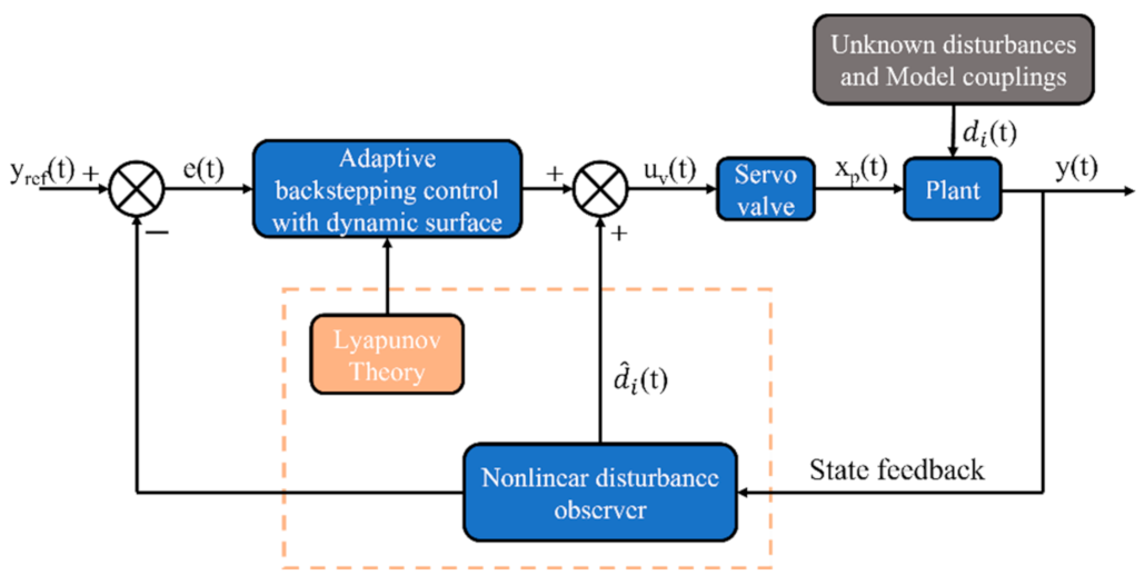
3. Control Design

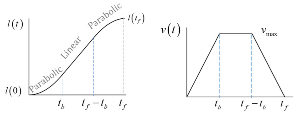
3.1. Trajectory Planning

Trajectory planning is the fundamental problem of the axial motion of deep-sea robots. The trajectory generation with given characteristics ensures that the robot can achieve the expected velocity and displacement within the specified time in the deep sea. The trajectories of the initial and final axial velocities are both zero, the first and last segments are parabolas, and the middle segment is linear. Then, the function of the axial motion is defined as

$$l(t)=\left\{\begin{array}{ll}l\left(0\right)+\frac{1}{2}\frac{v_{max}}{t_b}{t}^2& ,0<t\le t_b\\ l\left(0\right)-\frac{1}{2}{t}_b{v}_{max}+v_{max}t& ,t_b<t\le t_f-t_b\\ l\left(t_f\right)-\frac{1}{2}\frac{v_{max}}{t_b}{(t-t_f)}^2& ,t_f-t_b<t\le t_f\end{array}\right.$$

(15)

From Equation (15), the trapezoidal velocity of the system is symmetrical as shown in Figure 3, where the displacement at the middle time is equal to the average value of the displacement at the initial and final displacement, namely, $l\left(\frac{1}{2}{t}_f\right)=\frac{l\left(0\right)+l\left(t_f\right)}{2}$.

Figure 3. Motion curve.

3.2. Nonlinear Disturbance Observer

The disturbance observer observes and predicts various disturbances in the system and corrects the estimate according to the deviation of the estimated disturbance from the actual disturbance. The equation of state of a non-linear time-varying control system can be represented by states $x_1$ and $x_2$

$$\left\{\begin{array}{l}{\dot{x}}_1=x_2\\ {\dot{x}}_2=f(u,x_1,x_2,t)+d(t)\end{array}\right.$$

(16)

where $f$ represents a non-linear function of $x$, and $d(t)$ is the sum of the disturbances generated by the system coupling and the external unknown disturbances. Then, the estimated disturbance is designed to be

$$\left\{\begin{array}{l}\dot{z}(t)=-\sigma (x)x_2(t)-\sigma (x)[p(x)+f(u,x_1,x_2,t)]\\ \widehat{d}(t)=z(t)+p(x)\end{array}\right.$$

(17)

where $z(t)$ and $\sigma (x)$ represent the intermediate variables and the gains of estimated disturbances $\widehat{d}(t)$, respectively, and $p(x)$ can be designed as a nonlinear function, e.g., $\sigma (x)x_1$, ($\sigma (x)>0$). The observer gain $L$ can be designed as $L=\partial p/\partial x_1=\sigma (x)$. It is seen that the disturbance observer satisfies the exponential convergence condition, and thus the stability of the disturbance observer itself can be demonstrated. The nonlinear disturbance observer makes the entire system stable without relying on the higher-order differentiation of state variable $x_2$.

3.3. Controller Design

We expect the target to have zero robot vibration during the lifting and lowering of the robot, namely, $y_d=0$. However, the unknown interference is bounded, $\left|{\tilde{d}}_i\left(t\right)\right|\le {\overline{d}}_i,{\overline{d}}_i>0$. To simplify the process, the tracking error variable can be designed as $e_i=x_i-{\alpha }_i,i=1,\dots ,5$, and ${\alpha }_i$ is an intermediate control variable be designed as ${\alpha }_1=y_d$. A low-pass filter is designed to prevent the “complexity explosion” problem arising from repeated differentiation; ${\tau }_i{\dot{\alpha }}_i+{\alpha }_i={\overline{\alpha }}_i,{\alpha }_i(0)=0$, $0<{\tau }_i<1$, ${\overline{\alpha }}_i$, and ${\alpha }_i$ denote input and output variables, respectively.

Defining the filtering error as ${\tilde{\alpha }}_i$, we have ${\tilde{\alpha }}_i={\alpha }_i-{\overline{\alpha }}_i,{\dot{\tilde{\alpha }}}_i={\dot{\alpha }}_i-{\dot{\overline{\alpha }}}_i=-\frac{{\tilde{\alpha }}_i}{{\tau }_i}-{\dot{\overline{\alpha }}}_i$. Because ${\dot{\alpha }}_i$ is bounded $\left|{\dot{\alpha }}_i\right|\le B_i(x_1,x_2,x_3,x_4,y_d,y_d^{(i)}),B_i>0$, we apply Young’s inequality $ab\le \frac{1}{2}{a}^2+\frac{1}{2}{b}^2$, and then ${\tilde{\alpha }}_i{\dot{\tilde{\alpha }}}_i\le -\frac{1}{{\tau }_i}{\tilde{\alpha }}_i^2+\frac{{\tilde{\alpha }}_i^2{B}_i^2(x_1,x_2,x_3,x_4,y_d,y_d^{(i)})}{2\epsilon }+\frac{1}{2}\epsilon$, where $\epsilon$ represents a very small positive constant.

To enable the robot’s tracking error to converge to zero, we construct the Lyapunov function of the tracking error $e_1$ as $V_1(t)=\frac{1}{2}{e}_1^2$. Then, the derivative of $V_1(t)$ is ${\dot{V}}_1(t)=e_1{\dot{e}}_1=e_1({\dot{x}}_1-{\dot{y}}_d)=e_1(x_2-{\dot{y}}_d)$. Next, by designing virtual control variable ${\overline{\alpha }}_2=-c_1{e}_1+{\dot{y}}_d$, we obtain ${\dot{V}}_1(t)\le -c_1{e}_1^2+e_1{e}_2$, where $c_1$ is a positive constant. At the next design step, $e_2$ enables the inequality to hold. The Lyapunov function that constructs the tracking error $e_2$ is

$$V_2(t)=V_1(t)+\left(\frac{1}{2}{e}_2^2+\frac{1}{2}{\tilde{d}}_1^2(t)+\frac{1}{2{\gamma }_1}{\tilde{\delta }}_1^2(t)\right)$$

(18)

where ${\tilde{d}}_1(t)=d_1(t)-{\widehat{d}}_1(t)$, ${\gamma }_1$ is the design parameter, and ${\gamma }_1>0$. ${\tilde{\delta }}_1(t)$ indicates robust control parameters and is used to correct for the prediction error of unknown disturbances ${\tilde{d}}_1(t)$. The third and fourth terms in Equation (18) are applied to demonstrate the robustness of the nonlinear disturbance observer ${\widehat{d}}_1(t)$ and the adaptive law for the upper bound of the design disturbance error ${\tilde{\delta }}_1(t)$, respectively.

Taking the derivative of $V_2(t)$ yields ${\dot{V}}_2(t)=-c_1{e}_1{}^2+e_1{e}_2+e_2{\dot{e}}_2$. Taking the derivative of $e_2$, we receive ${\dot{e}}_2=e_3+{\alpha }_3+f_2(x_1,x_2,x_3)+d_1(t)-{\dot{\alpha }}_2$. Based on the nonlinear disturbance observer control theory, the virtual control variable ${\overline{\alpha }}_3$ is designed as

$${\overline{\alpha }}_3=-(c_2+\frac{1}{2})e_2-e_1-f_2(x_1,x_2,x_3)+{\dot{\alpha }}_2-{\widehat{d}}_1(t)-{\widehat{\delta }}_1(t)\mathrm{sign}\left(e_2\right)$$

(19)

where $c_2$ indicates a positive design constant. Bringing ${\overline{\alpha }}_3$ into Equation (19) and using Young’s inequality, the derivative of $V_2(t)$ is represented as

$${\dot{V}}_2(t)\le -c_1{e}_1{}^2-c_2{e}_2{}^2+e_2{e}_3+{\tilde{\delta }}_1(t)\left|e_2\right|+\frac{1}{2}{\tilde{\alpha }}_3{}^2$$

(20)

Because the estimated disturbance error ${\tilde{d}}_1(t)=d_1(t)-{\widehat{d}}_1(t)$ has a definite bounded error $\left|{\tilde{d}}_1(t)\right|\le {\delta }_1(t)$, we obtain

$${\dot{V}}_2(t)\le -c_1{e}_1^2-c_2{e}_2^2+e_2{e}_3+{\tilde{\delta }}_1(t)\left(\left|e_2\right|-\frac{1}{{\gamma }_1}{\dot{\widehat{\delta }}}_1(t)\right)-K_1{\tilde{d}}_1^2(t)+\frac{1}{2}{\tilde{\alpha }}_3^2$$

(21)

To guarantee the stability of the system and to minimize the prediction error, the updated law for the robust control parameter should be designed as ${\dot{\widehat{\delta }}}_1(t)={\gamma }_1\left|e_2\right|$. To ensure the boundedness of ${\widehat{\delta }}_1(t)$, the projection correction function is designed to replace the update of this control rate as follows

$${\mathrm{Proj}}_{\widehat{\delta }}\left(·\right)=\left\{\begin{array}{ll}0& \mathrm{if} {\widehat{\delta }}_i\ge {\delta }_{\max } \mathrm{and} ·>0\\ 0& \mathrm{if} {\widehat{\delta }}_i\le {\delta }_{\min } \mathrm{and} ·<0\\ ·& \mathrm{otherwise}\end{array}\right.$$

(22)

Applying Equation (22), the following inequality can be obtained: ${\tilde{\delta }}_1\left(·\right)\le {\tilde{\delta }}_1{\mathrm{Proj}}_{\delta }\left(·\right)$; then, Equation (21) is updated to ${\dot{V}}_2(t)\le -c_1{e}_1^2-c_2{e}_2^2+e_2{e}_3-K_1{\tilde{d}}_1^2(t)+\frac{1}{2}{\tilde{\alpha }}_3^2$. Similarly, design the dummy control variable ${\overline{\alpha }}_4$ as ${\overline{\alpha }}_4=-\left(c_3+\frac{1}{2}\right)e_3-e_2+{\dot{\alpha }}_3$. The Lyapunov function that constructs the tracking error $e_3$ is $V_3(t)=V_2\left(t\right)+\frac{1}{2}{e}_3{}^2$. Then, the derivative of $V_3(t)$ is ${\dot{V}}_3(t)={\dot{V}}_2(t)+e_3{\dot{e}}_3$. Bringing ${\overline{\alpha }}_4$ to ${\dot{V}}_3(t)$ and applying Young’s inequality, we receive

$${\dot{V}}_3(t)\le -c_1{e}_1^2-c_2{e}_2^2-c_3{e}_3^2+e_3{e}_4-K_1{\tilde{d}}_1^2(t)+\frac{1}{2}{\tilde{\alpha }}_3^2+\frac{1}{2}{\tilde{\alpha }}_4^2$$

(23)

Similarly, from the disturbance observer control theory, the virtual control variable ${\overline{\alpha }}_5$ is designed as

$${\overline{\alpha }}_5=\frac{1}{b_4}\left(-\left(c_4+\frac{1}{2}\right)e_4-e_3-f_4\left(x_1,x_3,x_4\right)-{\widehat{d}}_2(t)-{\widehat{\delta }}_2\mathrm{sgn}\left(e_4\right)+{\dot{\alpha }}_4\right)$$

(24)

The Lyapunov function for the construction of tracking error $e_4$ is

$$V_4(t)=V_3(t)+\left(\frac{1}{2}{e}_4^2+\frac{1}{2}{\tilde{d}}_2^2(t)+\frac{1}{2{\gamma }_2}{\tilde{\delta }}_2^2(t)\right)$$

(25)

where ${\tilde{d}}_2(t)=d_2(t)-{\widehat{d}}_2(t)$, ${\gamma }_2$ is the design parameter, and ${\gamma }_2>0$. ${\tilde{\delta }}_2(t)$ indicates a robust control parameter and is used to correct for the estimation error of unknown disturbances ${\tilde{d}}_2(t)$. The third and fourth terms in Equation (25) are applied to demonstrate the stability of the nonlinear disturbance observer ${\widehat{d}}_2(t)$ and the updated law for the upper bound of the design disturbance error ${\tilde{\delta }}_2(t)$, respectively.

Taking the derivative of $V_4(t)$ yields ${\dot{V}}_4(t)={\dot{V}}_3(t)+e_4{\dot{e}}_4$. However, taking the derivative of $e_4$, we obtain ${\dot{e}}_4=b_4{e}_5-\left(c_4+\frac{1}{2}\right)e_4-e_3+{\delta }_2\left(t\right)-{\widehat{\delta }}_2\mathrm{sgn}\left(e_4\right)$. Additionally, applying Young’s inequality, we receive

$${\dot{V}}_4(t)={\dot{V}}_3(t)+b_4{e}_4{e}_5-\left(c_4+\frac{1}{2}\right)e_4^2-e_3{e}_4+{\widehat{\delta }}_2(t)e_4\mathrm{sgn}(e_4)+{\tilde{d}}_2(t){\dot{\tilde{d}}}_2(t)+\frac{1}{{\gamma }_2}{\tilde{\delta }}_2(t){\dot{\tilde{\delta }}}_2(t)$$

(26)

Similarly, to guarantee the stability of the system and to minimize the prediction error, the updated law for the robust control parameter should be designed as ${\dot{\widehat{\delta }}}_2(t)={\gamma }_2\left|e_4\right|$. In order to ensure the boundedness of ${\widehat{\delta }}_2(t)$, the projection correction function (22) is applied to replace the update of this control rate, then Equation (26) can be rewritten as

$${\dot{V}}_4(t)\le -{\displaystyle \sum _{i=1}^4{c}_i{e}_i^2}+b_4{e}_4{e}_5-K_1{\tilde{d}}_1^2(t)-K_2{\tilde{d}}_2^2(t)+\frac{1}{2}{\displaystyle \sum _{i=3}^5{\tilde{\alpha }}_i^2}$$

(27)

The final design control input is

$$u_v=\frac{1}{b_5}\left(-\left(c_5+\frac{1}{2}\right)e_5-b_4{e}_4-f_5(x_4,x_5)+{\dot{\alpha }}_5\right)$$

(28)

The Lyapunov function that constructs the tracking error $e_5$ is $V_5(t)=V_4(t)+\frac{1}{2}{e}_5^2$. Taking the derivative of $V_5(t)$ and applying Young’s inequality yields

$${\dot{V}}_5(t)\le -{\displaystyle \sum _{i=1}^4{c}_i{e}_i^2-\left(c_5+\frac{1}{2}\right)e_5^2-K_1{\tilde{d}}_1^2(t)-}{K}_2{\tilde{d}}_2^2(t)+\frac{1}{2}{\displaystyle \sum _{i=3}^5{\tilde{\alpha }}_i^2}$$

(29)

The adaptive robust controller was designed earlier according to Lyapunov theory, where NDO is used to compensate for the rigid–flexible coupling and unknown perturbations of the system, which can be seen in Figure 4. Additionally, the stability of the closed-loop system was proved subsequently.

Figure 4. Control scheme.

3.4. Stability Analysis

To demonstrate that the above control scheme is feasible, the stability of the control system is now proved by constructing the Lyapunov function of the system as

$$V(t)=\frac{1}{2}{\displaystyle \sum _{i=1}^5{c}_i{e}_i^2+\frac{1}{2}{\tilde{d}}_1^2(t)+}\frac{1}{2}{\tilde{d}}_2^2(t)+{\displaystyle \sum _{i=1}^2\frac{1}{{\gamma }_i}}{\tilde{\delta }}_i^2(t)+\frac{1}{2}{\displaystyle \sum _{i=2}^5{\tilde{\alpha }}_i^2(t)}$$

(30)

Taking the derivative for $V(t)$ and using the above series of inequalities yields

$$\dot{V}\left(t\right)\le -{\displaystyle \sum _{i=1}^5{c}_i{e}_i^2-K_1}{\tilde{d}}_1^2(t)-K_2{\tilde{d}}_2^2(t)-{\displaystyle \sum _{i=2}^5\left(\frac{1}{{\tau }_i}-\frac{1}{2}-\frac{B_i^2}{2\epsilon }\right){\tilde{\alpha }}_i^2(t)}$$

(31)

To ensure that $V(t)$ is non-negative and $\dot{V}\left(t\right)$ is non-positive, the constants $c_i,K_i,{\tau }_i$ should satisfy the following conditions $c_i>0,K_i>0,\frac{1}{{\tau }_i}-\frac{1}{2}-\frac{B_i^2}{2\epsilon }>0$. When $k_0$ satisfies the condition $\left\{2c_i>0,2K_i>0,2\left(\frac{1}{{\tau }_i}-\frac{1}{2}-\frac{B_i^2}{2\epsilon }\right)\right\}>0$, Equation (31) can be rewritten as

$$\dot{V}\left(t\right)\le -k_{0}V\left(t\right)$$

(32)

Multiplying the above equation by $e^{k_{0}t}$ and integrating over the time domain $[0,t)$ gives $V\left(0\right)\le e^{-k_{0}t}V\left(0\right)$. Because the Lyapunov function $V\left(t\right)$ of tracking error $e_1,e_2,e_3,e_4,e_5$ converges, $e_1$ converges to zero with time based on Barbalat Lemma [27].

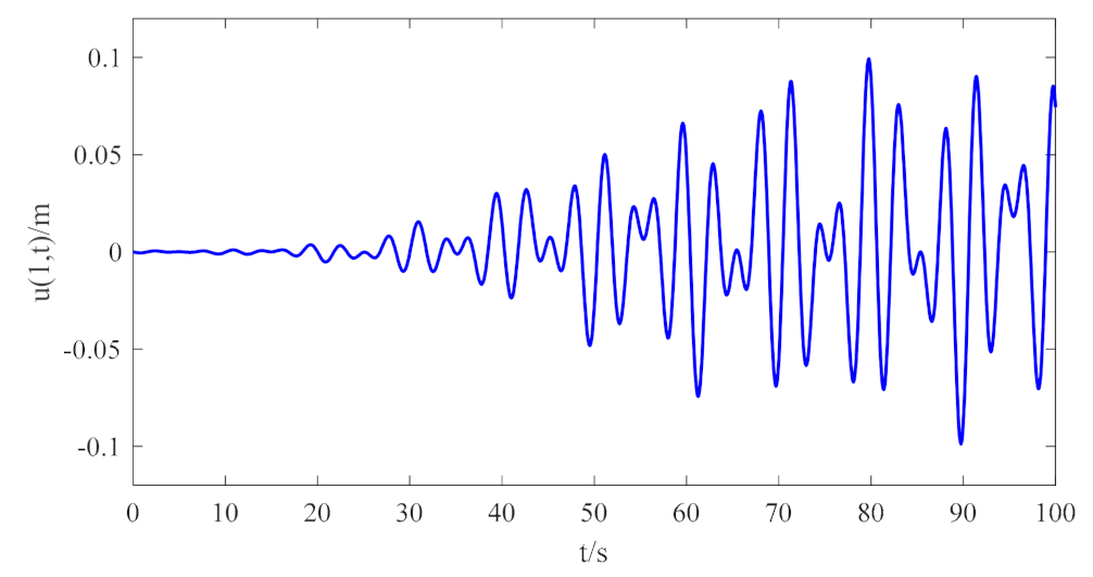
4. Simulation Results

To verify the effectiveness of the controller proposed in the previous section, the key technical parameters of the deep-ocean robotic compensation system are selected as follows: $m_p=2000$ kg, $EA=2\times {10}^7$ N, ${\rho }_l=2$ kg/m, and $c=10$ Ns/m². The initial length of the umbilical cable is 10 m, and the final length is 1000 m. The umbilical cable and the robot are initially static: $u\left(x,0\right)=0$ m and $u_t\left(x,0\right)=0$ m/s. The key physical parameters of the system are selected as $m_t=500$ kg, $\rho =900$ kg/m³, $A_p=0.01767$ m², $k_v=1$, $C_d=0.7$, $w_v=0.002$, $C_{tp}=2.3\times {10}^{-10}$ m³/(s·pa), $B_p=7500$, $p_s=15$ Mpa, and ${\beta }_e=1.2\times {10}^9$ pa.

The hydraulic cylinder piston is initially in the neutral position $x_p=0$ m, and the servo valve spool is in the zero position $x_v=0$ m. The piston of the hydraulic cylinder is subjected to the disturbing force of waves on the sea’s surface, which can be expressed as $d_t\left(t\right)=1.4\sin \left(0.5\pi t\right)+1.6\sin \left(0.7\pi t\right)$, and the robot is subjected to random disturbances on the sea floor, which can be expressed as $d_p\left(t\right)=1.6\sin \left(2\pi t/13\right)$. Without control, the numerical solution of Equation (4) is obtained using the Runge–Kutta method, and then the approximate response of the system is given in Figure 5.

Figure 5. Robot vibration displacement without control.

The diagram clearly shows the vibration of the robot at the balance position becomes more significant with the increasing length of the umbilical cable, and the results are consistent with the previous analysis. In deep-sea operations, factors such as varying sea conditions and depths have different significant effects concerning the control performance of the compensation system. Therefore, the paper uses boundary disturbances under two waves to simulate extreme environments and verify the controller performance.

Based on the above stability analysis and several simulation tests, the design parameters are set for the controller: $c_1=42$, $c_2=20$, $c_3=4$, $c_4=2$, $c_5=100$, ${\tau }_i=0.01$, $\epsilon =0.21$, ${\gamma }_1={\gamma }_2=0.002$, and $L=80$. The upper bound of the robust term ${\widehat{\delta }}_i$ is set to ${\delta }_{\max }=0.01$ and the lower bound is set to ${\delta }_{\min }=0$. Figure 6, Figure 7, Figure 8, Figure 9 and Figure 10 give the simulation results, respectively.

Figure 6. Underwater robot boundary disturbance force.

Figure 7. Hydraulic compensation system boundary disturbance force.

Figure 8. Performance comparison of active heave compensation.

Figure 9. Hydraulic cylinder piston displacement.

Figure 10. Control input voltage of the servo valve.

Figure 6 shows the boundary disturbance to the deep-sea robot simulated by random waves. Figure 7 shows the boundary disturbance to the hydraulic compensator affected by the superposition of several different periodic delta function waves. It is noticeable from the figure that the nonlinear disturbance observer has an excellent estimation performance.

The active compensation results of the deep-ocean robot under the proposed nonlinear disturbance observer-based and robust adaptive output feedback controls are displayed in Figure 8. From the graph, it is noticeable that the effect of PID control gradually becomes worse with the increased length of the umbilical cable, whereas the control scheme suggested above can effectively suppress vibration. The vibration amplitude gradually converges to zero as time increases. Additionally, the maximum compensation error of the PID controller is about 2.2 mm, whereas the maximum compensation error of the controller proposed in this paper is about 0.1 mm. From Figure 6 and Figure 7, the nonlinear disturbance observer enables the online estimation of disturbances and achieves satisfactory estimation performance. Figure 9 and Figure 10 show the piston rod displacement and control input voltage of the servo valve, respectively. From this, the maximum piston displacement under PID control is approximately 33 mm more than the control scheme proposed in this paper, and the PID control input voltage may exceed the maximum input voltage over time and oscillate, with harmful effects on the vibration rejection of the robot. Therefore, the robust controller proposed above has a superior performance over conventional PID control in terms of the effectiveness and robustness of the active heave compensation of the robot.

5. Conclusions

The robust adaptive output feedback control scheme has been designed for a type of active heave compensation system for deep-ocean robots with variable length, non-linearity, and uncertain random disturbances. Second-order distributed parameter control equations for the umbilical rope lifting system were established using Hamilton’s principle, and the equations were discretized by a newly modified assumption modal method, according to Newton’s second law, which couples valve-controlled hydraulic cylinder compensation systems and generates the state space equation of the system. A nonlinear disturbance observer has been proposed to overcome the unknown disturbances and input nonlinearity, followed by a simplified description of the design route of the adaptive robust control algorithm and the stability validation of the system based on Lyapunov’s direct method and cascade analysis. A comparison of different control effects shows that an increase in the length of the umbilical cable leads to an increase in the robot’s heave displacement, and the proposed controller is more applicable for robot heave compensation. The different control results demonstrate the performance of the robust adaptive backstepping control strategy, and the suggested controller can achieve better robustness and stability of the system at the right choice of control gain. In the future, more accurate hydraulic compensation models and larger compensation depths will be considered to improve active heave compensation accuracy.

References

- Wu, N.L.; Wang, X.Y.; Ge, T.; Wu, C.; Yang, R. Parametric identification and structure searching for underwater vehicle model using symbolic regression. J. Mar. Sci. Technol. 2017, 22, 51–60. [Google Scholar] [CrossRef]
- Azis, F.A.; Aras, M.S.M.; Rashid, M.Z.A.; Othman, M.N.; Abdullah, S.S. Problem identification for underwater remotely operated vehicle (ROV): A case study. Procedia Eng. 2012, 41, 554–560. [Google Scholar] [CrossRef]
- Jiang, C.M.; Wan, L.; Sun, Y.S. Design of motion control system of pipeline detection AUV. J. Cent. South Univ. 2017, 24, 637–646. [Google Scholar] [CrossRef]
- Petillot, Y.R.; Antonelli, G.; Casalino, G.; Ferreira, F. Underwater robots: From remotely operated vehicles to intervention-autonomous underwater vehicles. IEEE Robot. Autom. Mag. 2019, 26, 94–101. [Google Scholar] [CrossRef]
- Woodacre, J.K.; Bauer, R.J.; Irani, R.A. A review of vertical motion heave compensation systems. Ocean Eng. 2015, 104, 140–154. [Google Scholar] [CrossRef]
- Quan, W.; Liu, Y.; Zhang, Z.; Li, X.; Liu, C. Scale model test of a semi-active heave compensation system for deep-sea tethered ROVs. Ocean Eng. 2016, 126, 353–363. [Google Scholar] [CrossRef]
- Lubis, M.B.; Kimiaei, M.; Efthymiou, M. Alternative configurations to optimize tension in the umbilical of a work class ROV performing ultra-deep-water operation. Ocean Eng. 2021, 225, 108786. [Google Scholar] [CrossRef]
- Woodacre, J.K.; Bauer, R.J.; Irani, R. Hydraulic valve-based active-heave compensation using a model-predictive controller with non-linear valve compensations. Ocean Eng. 2018, 152, 47–56. [Google Scholar] [CrossRef]
- Ren, Z.; Skjetne, R.; Verma, A.S.; Jiang, Z.; Gao, Z.; Halse, K.H. Active heave compensation of floating wind turbine installation using a catamaran construction vessel. Mar. Struct. 2021, 75, 102868. [Google Scholar] [CrossRef]
- Liu, J.; Zhao, H.; Liu, Q.; He, Y.; Wang, G.; Wang, C. Dynamic behavior of a deepwater hard suspension riser under emergency evacuation conditions. Ocean Eng. 2018, 150, 138–151. [Google Scholar] [CrossRef]
- Lee, D.H.; Kim, T.W.; Ji, S.W.; Kim, Y.B. A study on load position control and vibration attenuation in crane operation using sub-actuator. Meas. Control. 2019, 52, 794–803. [Google Scholar] [CrossRef]
- Li, S.; Wei, J.; Guo, K.; Zhu, W.L. Nonlinear robust prediction control of hybrid active–passive heave compensator with extended disturbance observer. IEEE Trans. Ind. Electron. 2017, 64, 6684–6694. [Google Scholar] [CrossRef]
- Gu, P.; Walid, A.A.; Iskandarani, Y.; Karimi, H.R. Modeling, simulation and design optimization of a hoisting rig active heave compensation system. Int. J. Mach. Learn. Cybern. 2013, 4, 85–98. [Google Scholar] [CrossRef]
- Cao, Y.; Wen, C.; Song, Y. Prescribed performance control of strict-feedback systems under actuation saturation and output constraint via event-triggered approach. Int. J. Robust Nonlinear Control. 2019, 29, 6357–6373. [Google Scholar] [CrossRef]
- Qu, Z. Robust Control of Nonlinear Uncertain Systems; John Wiley & Sons, Inc.: Hoboken, NJ, USA, 1998. [Google Scholar]
- Xing, X.; Liu, J. Modeling and robust adaptive iterative learning control of a vehicle-based flexible manipulator with uncertainties. Int. J. Robust Nonlinear Control. 2019, 29, 2385–2405. [Google Scholar] [CrossRef]
- Islam, S.; Liu, X.P. Robust sliding mode control for robot manipulators. IEEE Trans. Ind. Electron. 2010, 58, 2444–2453. [Google Scholar] [CrossRef]
- Li, Z.; Ma, X.; Li, Y.; Meng, Q.; Li, J. ADRC-ESMPC active heave compensation control strategy for offshore cranes. Ships Offshore Struct. 2020, 15, 1098–1106. [Google Scholar] [CrossRef]
- Yu, H.; Chen, Y.; Shi, W.; Xiong, Y.; Wei, J. State constrained variable structure control for active heave compensators. IEEE Access 2019, 7, 54770–54779. [Google Scholar] [CrossRef]
- Kwon, S.; Chung, W.K. A discrete-time design and analysis of perturbation observer for motion control applications. IEEE Trans. Control. Syst. Technol. 2003, 11, 399–407. [Google Scholar] [CrossRef]
- Chen, W.H.; Yang, J.; Guo, L.; Li, S. Disturbance-observer-based control and related methods—An overview. IEEE Trans. Ind. Electron. 2015, 63, 1083–1095. [Google Scholar] [CrossRef]
- Li, S.; Yang, J.; Chen, W.H.; Chen, X. Generalized extended state observer based control for systems with mismatched uncertainties. IEEE Trans. Ind. Electron. 2011, 59, 4792–4802. [Google Scholar] [CrossRef]
- Sun, N.; Yang, T.; Chen, H.; Fang, Y. Dynamic feedback antiswing control of shipboard cranes without velocity measurement: Theory and hardware experiments. IEEE Trans. Ind. Inform. 2018, 15, 2879–2891. [Google Scholar] [CrossRef]
- Swaroop, D.; Hedrick, J.K.; Yip, P.P.; Gerdes, J.C. Dynamic surface control for a class of nonlinear systems. IEEE Trans. Autom. Control. 2000, 45, 1893–1899. [Google Scholar] [CrossRef]
- Kim, S.K.; Ahn, C.K.; Shi, P. Performance recovery tracking-controller for quadcopters via invariant dynamic surface approach. IEEE Trans. Ind. Inform. 2019, 15, 5235–5243. [Google Scholar] [CrossRef]
- Shi, M.; Guo, S.; Jiang, L.; Huang, Z. Active-passive combined control system in crane type for heave compensation. IEEE Access 2019, 7, 159960–159970. [Google Scholar] [CrossRef]
- Hou, M.; Duan, G.; Guo, M. New versions of Barbalat’s lemma with applications. J. Control. Theory Appl. 2010, 8, 545–547. [Google Scholar] [CrossRef]