Article

A Decision-Making Tool for Port Operations Based on Downtime Risk and Met-Ocean Conditions including Infragravity Wave Forecast

Water and Environmental Engineering Group (GEAMA), University of A Coruña, 15071 A Coruña, Spain
*
Author to whom correspondence should be addressed.
J. Mar. Sci. Eng. 2023, 11(3), 536; https://doi.org/10.3390/jmse11030536
Submission received: 2 February 2023 / Revised: 23 February 2023 / Accepted: 28 February 2023 / Published: 1 March 2023
(This article belongs to the Special Issue Design of Harbour and Coastal Structures)

Abstract

:
Port downtime leads to economic losses and reductions in safety levels. This problem is generally assessed in terms of uni-variable thresholds, despite its multidimensional nature. The aim of the present study is to develop a downtime probability forecasting tool, based on real problems at the Outer Port of Punta Langosteira (Spain), and including infragravity wave prediction. The combination of measurements from three pressure sensors and a tide gauge, together with machine-learning techniques, made it possible to generate long wave prognostication at different frequencies. A fitting correlation of 0.95 and 0.9 and a root mean squared error (RMSE) of 0.022 m and 0.012 m were achieved for gravity and infragravity waves, respectively. A wave hindcast in the berthing areas, met-ocean forecast data, and information on 15 real operational problems between 2017 and 2022, were all used to build a classification model for downtime probability estimation. The proposed use of this tool addresses the problems that arise when two consecutive sea states have thresholds above 3.97%. This is the limit for guaranteeing the safety of port operations and has a cost of just 0.6 unnecessary interruptions of operations per year. The methodology is easily exportable to other facilities for an adequate assessment of downtime risks.

1. Introduction

During port operations, moored ships may experience excessive movement or high stresses on lines, which can restrict the performance of (un)loading, a period known as downtime. In some scenarios, the mooring becomes unsafe and leads to a vessel being evacuated from its berth, which is also considered downtime [1]. Such incidents imply economic loss for the owners of the port facilities, agents, and shipping companies, as well as reductions in safety levels [2]. Investment in more effective operability management systems may improve this situation [3] and lead to more sustainable ports, in terms of both environmental and social impacts [4].
Extreme vessel motion and line pre-tension are caused by met-ocean conditions. In ports exposed to swell, wave heights are closely related to operational problems [5]. However, other factors, such as wind, currents, and sea level, can also have an influence. Thus, port operability is traditionally studied in relation to the limits of climatic variables and the maximum amplitudes of the different moored ships’ movements. Different thresholds are established, depending on ship type and the cargo-handling equipment. The criteria for met-ocean factors are set out in [6,7]; the values for defining allowable ship motion for each of a vessel’s six degrees of freedom are presented in [8,9].
These limits are used in the assessment of downtime with respect to the behavior of a particular vessel berthed in a specific port [10,11,12]. For this reason, the response of the ship-lines-fenders system is sometimes simulated with a numerical model and recently additionally through machine-learning tools [13,14].
Corresponding thresholds are also applied for operational analysis based on met-ocean conditions. Most of these refer to a single indicator such as short waves [15,16], long waves [17], or wind [18]. Recently, these limits have also been used to assess port operability from the perspective of the impact of climate change [19,20,21,22]. Some analyses use a criterion conditioned by two variables [23,24]. The latter study highlights the fact that, irrespective of this, the decision to suspend operations continues to depend on the perception of vulnerability by operators and captains.
Infragravity waves affect horizontal movements, which can significantly increase downtime [25]. In [26] long-wave thresholds are proposed for operability problems, although it remains a uni-variable limit applied to a specific ship typology. This climatic variable is not commonly available, but various authors have been able to forecast it based on short-wave data and machine-learning techniques [2,15,27].
While many ports have climate forecasts, obtaining information on vessel movements is complex due to the computational cost and the need for validation. Moreover, thresholds are defined for each different parameter. However, the problem here involves the interaction of various factors: met-ocean forcings, a moored floating body with six degrees of freedom (DoF), cargo handling, and the human factor (taking into account the subjectivity of the perception of danger). Recent research has highlighted the multivariate influence of downtime assessment, including infragravity waves [24,28]. It should be noted that movement restrictions and the human factor are not predictable, as both depend on personal perspectives.
Multi-criteria decision-making models (MCDM) are applied in various fields. The combination of DEA window analysis with the Malmquist index approach was used to assess the efficiency of the cybersecurity industry [29] or to express the linguistic evaluation statements of experts [30]. In applying these ideas to the present topic, we were able to confirm that the contribution to this area of knowledge is significant.
Considering the above, this study presents a multidimensional methodology to predict downtime risk based on climatic forecast data, including the development of a gravity and infragravity wave forecast, as applied to the Outer Port of Punta Langosteira. In these facilities, the cargo handling equipment is the same for all the vessels it currently receives (port cranes on wheels). Therefore, it constitutes an accessible methodology, which can be easily exported to other ports. The main aim of the work is to develop a tool to help predict the operational problems of bulk carriers and general cargo vessels. Actual downtime data from 2017 to 2022 for the docks in question, together with met-ocean forecast data, were used. Additionally, in order to include long waves, a field campaign was conducted to obtain records in five berthing areas. Several methods were compared for obtaining the optimal wave height forecast in the different frequency bands in the basin. For this purpose, in addition to waves, data on sea level, wind, and the NAO index were also included.
The remainder of the paper is structured as follows: Section 2 introduces the study area, the data used, and the methodology. Section 3 presents a comparison of different approaches for significant wave height forecasts at different frequencies, and reports on the results of the downtime prediction model. Finally, conclusions are offered in Section 4.

2. Materials and Methods

In this section the study area is presented, together with the prevailing climatic conditions. In addition, the field campaign data and the methodologies applied to the forecast of waves and downtime probability are described.

2.1. Study Area

The Outer Port of Punta Langosteira (A Coruña, Spain) is located in north-western Spain (43°21′27.6″ N; 8°23′13.7″ W) (Figure 1a,b). This harbor has a sheltered area of 264 Ha with a 3360 m breakwater, developed in three alignments, and a 1327 m secondary breakwater in two alignments (Figure 1c). Within the port there is a 1560 m continuous multipurpose dock, 950 m of which has an average draft of 21 m (zones: Z4, Z5 and Z6), 445 m has a depth of 15 m (zone Z3), and there is an intermediate draft transition zone of 16.5 m (A2 dock). Current traffic carries bulk solids and general cargo, and after the completion of the ongoing construction of the new jetty, the unloading of liquid bulk will begin at the facility. The jetty consists of 19 precast concrete caissons with space for three vessels of up to 300 m and 200,000 tons (Suezmax). Two other infrastructures of similar sizes are also planned.
Spain’s Atlantic coast has a very high operability risk level in worldwide terms [31]. The most energetic storms have directions in the NW-NNW range, reaching significant wave heights (Hs) of an extreme regime, exceeding 10 m, and with wave peak periods (Tp) of up to 22 s. In addition, the maximum tide range is 4.5 m. Under these conditions, knowledge of the situations in which downtime events occur is key to optimizing operability and the safety of operations.

2.2. Field Campaign

In order to obtain short- and long-wave information at the different berths for forecasting purposes, a field campaign was carried out between December 2021 and April 2022. Six pressure sensors TRAFAG ECL1.0AP model of 1 bar were installed at the locations shown in Figure 1c (S1, S2, S3, S4, S5 and S6). It should be noted that S2 was lost before its data could be collected, and hence could not be used in the study. These sensors were equipped with dataloggers, batteries, and software created ad hoc for their automatic synchronization, through internet connections via SIM cards and data storage with a recording frequency of 4 Hz. The equipment was designed to operate autonomously for at least one month, without the need to replace batteries. In addition, the records of the Miros radar tide gauge model, which forms part of the Tide Gauges Network of the Spanish Port Authority [32] (REDMAR, code 3214), were used.
Date and time information for 15 downtime events that occurred in the period 2017–2022 on bulk carriers and general cargo vessels between 89 m and 180 m in length was available (Table 1). There were eight operational downtime events (operability) and seven further ones which resulted in vessel evacuation from the berth (safety). These data were used in [28] for the analysis of the influence of various climatic variables. As in that study, the hours in which operations were suspended, together with the two hours prior to the evacuation of the vessel, are used to indicate the presence of the problems.
The met-ocean information used to define each sea state (1 h) was from the port forecast (Cuadro de Mando Ambiental—Harbor Environmental Monitoring Dashboard: http://cma.puertocoruna.com/ (accessed on 3 January 2023)) at the Langosteira II buoy location (43.35° N 8.56° W) (Figure 1b), which forms part of the Coastal Buoy Network of the Spanish Port Authority (REDCOS) [32]. These variables were significant wave height (Hs), peak period (Tp), wave direction (Dir), wind velocity (Vw) and direction (Dirw), together with sea level data at the tide gauge location (Figure 1c).

2.3. Gravity and Infragravity Waves Forecast

A regression model was applied to obtain the significant short- and long-wave heights in the vicinity of the berths. Additionally, a comparison was made of the results of the model with the fit to the empirical formulation. Both methods are described in this section, together with the variables involved.

2.3.1. Input and Output Parameters

To achieve a fit of any model, the expected results need to be known beforehand. Therefore, the significant wave height (Hs) was calculated for each frequency band of the pressure sensor and tide gauge signal. To do this, a window filter was applied to the signals in order to obtain the time series between the periods under investigation. Four ranges were defined: swell (1–30 s); low infragravity waves (LIG) (30–70 s); up infragravity waves (UIG) (70–150 s) and far infragravity waves (FIG) (150–300 s). From these filtered records, significant wave heights were estimated for each sea state as the average of the largest third amplitudes, that is, the differences between peaks and valleys identified by zero-crossing.
The presence of long waves in a harbor is mainly due to the nonlinear wave interactions in the propagation [27,33,34,35,36] and to atmospheric disturbances [37,38,39]; in addition, transient long waves are common external triggering forces [40,41]. Considering the first-generation mechanism, the significant wave height (Hs), peak period (Tp) and direction (Dir) outside the port, as well as the tide level within the basin, were used to forecast the infragravity waves at the different frequencies. To add information relating to atmospheric disturbances, wind speed (Vw) and direction (Dirw), the North Atlantic Oscillation (NAO) index was introduced.
The latter mechanism is a novelty in addressing a problem such as the one here. However, some authors have investigated the relationship between climate indices and shoreline change [42,43], even looking directly at waves [44]. In particular, in [45] the correlation between the swell off the Galician coast (NW Spain) and the NAO index is explored.
The NAO is the climate variability in the North Atlantic. This index provides information on weather phenomena over the North Atlantic Ocean by assessing the difference in sea level pressures between two points over the ocean: the permanent low-pressure system over Iceland (the Icelandic Low) and the permanent high-pressure system over the Azores (the Azores High) [46]. A positive NAO index implies a reduction in atmospheric pressure, which leads to a rise in sea level. These barometric effects generate a level gradient, which can be the cause of sea surface oscillations. For the present study, this daily index, which is available at https://ftp.cpc.ncep.noaa.gov/cwlinks/ (accessed on 2 January 2023), was transformed to hourly data in order to assign a value to each sea state under consideration.

2.3.2. Empirical Formulation to Compute Infragravity Waves Heights

Historically, the way of estimating a variable involved building a model using theoretical concepts, and its parameters were then fitted according to the observed data. A number of formulations are available in the literature to predict the height of infragravity waves from swell waves [47,48,49]. Based on the procedures of these previous studies, the first estimation of the long waves in the port was obtained by fitting it to the field data through the well-known [46] formula:
H s = k H s α T p β d γ
where k, α, β and γ are site-specific empirical parameters, Hs is the significant wave height, Tp is the peak period, and d is the depth considering the tide level. The symbol “-” refers to the frequency band (LIG (30–70 s), UIG (70–150 s) or FIG (150–300 s).

2.3.3. Regression Model

In some real situations, the formulations are not available or do not permit the addition of new variables towards improving the results. These problems can be avoided if non-parametric machine-learning techniques are applied, since they allow for the construction of a model directly from the data, without the need to know the relationships between the parameters. These have already been used in the prediction of significant wave heights with excellent results [2,50]. In the present study, certain findings are made with respect to the existing literature, including new atmospheric variables and the utilization of forecast data, raising a further problem in that the latter differ from reality on some occasions.
Based on the defined parameters, a gradient boosting machine (GBM) was employed to estimate the short and long waves in the different frequency bands in each berthing area. This algorithm can be used to build a non-parametric regression or classification model from the data. Therefore, it was also applied for downtime forecasting with the necessary peculiarities involved.
The learning procedure of this algorithm is to generate a model that sequentially builds trees that provide a more accurate estimation of the output variable. To this end, it performs multiple iterations, and in each of these it builds a tree that evaluates the residuals of the previous iteration, thus involving a consecutive fitting of errors. These are obtained by minimizing the loss function, the choice of which depends on the researcher [51,52]. In this case, the Gaussian distribution was applied:
w   y f 2
where w is the weight, y is a true response, and f is a predicted response) [53]. For the determination of the hyperparameters that reduce the loss function, the root mean squared error (RMSE) was used as a metric.
A common problem in machine-learning techniques is overfitting. This was solved by implementing a regularization procedure consisting of cross-validation combined with early stopping. The data were divided into j = 10 disjoint non-overlapping subsets. One of the j sets was reserved and the others were used for fitting the GBM. Subsequently, the model was validated with the reserved fold to obtain the predictive performance. In this training, when the difference in the validation error with respect to the previous iteration was very small, it was stopped (early stopping), with the previous step achieved considered to be optimal. This was repeated by reserving a subset each time. Finally, the behavior of the model was obtained as the average of the RMSE of each j fold.

2.4. Downtime Risk Forecast

To achieve the main objective, a classification model was developed to predict downtimes. The variables used and the main characteristics of its application are described below.

2.4.1. Input and Output Parameters

The data used here were the forecast parameters that define the sea states (Hs, Tp, Dir, Vw, Dirw, tide level) together with NAO index and the short and long waves in each berthing area, this during the months of October to April, 2017–2022. It should be noted that only information between 7 a.m. and 8 p.m. was selected, as port operators generally do not work at night, and hence operational downtime events cannot be detected at these times. Likewise, periods in which no vessels were berthed at the port were disregarded.
To obtain data on significant wave heights in all the frequency ranges described, a hindcast was performed with the regression model, this corresponding to the sea states under study in the downtime forecast.
In addition to these climatic data, a column was added to identify the problems in each sea state: all the hours with operational stoppage and the two hours prior to berth evacuation.

2.4.2. Classification Model

Gradient boosting machines (GBMs) are a family of powerful supervised learning techniques that have achieved considerable success in a variety of applications. One great advantage is their high level of customization for the needs of a specific task through the choice of the most suitable loss function.
As discussed above, the GBM used in the present study optimizes predictive results through increasingly refined approximations by sequentially building models on the characteristics of the data set. In this case it was also applied with cross-validation and early stopping, as discussed in Section 2.3.3. By contrast, the fitting was carried out with the recommended loss function for classification models, that is, the Bernoulli distribution:
2 w y · log f + 1 y · log 1 f
where w is the weight, y is a true response, and f is a predicted response [53]. The output obtained was the downtime probability for each sea state, which was used to analyze the optimal threshold for support in decision-making.
To sum up, Figure 2 shows the workflow that links the result of the regression model with the classification model to obtain the wave heights at the different frequencies and ultimately the downtime probability.

3. Results and Discussion

The performance of the tools developed is presented here. The first Section 3.1 sets out and compares the results of the prediction of the significant short- and long-wave height at the different berths; the second part Section 3.2 discusses the output of the downtime risk forecasting model, in which the result of the first section is used as an input variable.

3.1. Gravity and Infragravity Waves Forecast

In order to choose the optimal model and variables for wave forecasting, a comparison was made of the results obtained from the tide gauge records with the empirical formula and the machine-learning model. The latter was applied with different input variables: first, significant wave height, peak period and tide level (as well as the formula); second, the purely oceanic factors (Hs, Tp, wave direction and tide level); and finally, all of the above together with the atmospheric parameters (wind speed and direction, and the NAO index).
The values of the four coefficients of Equation (1) (k, α, β and γ) were calculated using nonlinear least squares for the three frequency bands under study. To do this, the significant wave heights of each period range of the tide gauge and the forecast of Hs and Tp at the buoy location were used. The results are presented in Table 2, together with those of other authors’ estimates at several European facilities.
Except for the values of k and γ for Hs of 150–300 s, the coefficients are in the same order of magnitude in all frequency ranges at the Outer Port of Punta Langosteira. They are also similar to those calculated by other authors elsewhere, except for γ, which was negative in the 30–70 s and 70–150 s bands. This may be due to the difference in draft of this large outer harbor (around 20 m at berth) since it directly modifies depth.
In order to compare the performance of the formula and the model, Table 3 shows the correlation coefficient (R2) and RMSE obtained for each option. The statistics in the different period bands achieved with the tide gauge data are also presented. The slight improvement in the model compared to the formula using only the variables Hs, Tp and tide level (1% of the R2) can be observed. The high correlation obtained in both cases indicates the influence of the short wave on the long wave, with the consequence that the latter is considered the bound wave. However, when the wave direction is added, the increase in this coefficient is 5% and 3% for gravity and infragravity waves, respectively. Finally, the application of the GBM with oceanic and atmospheric parameters (wind speed and direction, and NAO index) was enriching, leading to an increase in the correlation of more than 2.5% on average. Therefore, the methodology proposed here improves the fitting with respect to the empirical formula by more than 6% and reduces the RMSE by more than 0.004 m of the significant long wave height on average (30%, 28% and 18% in the LIG, UIG and FIG bands, respectively).
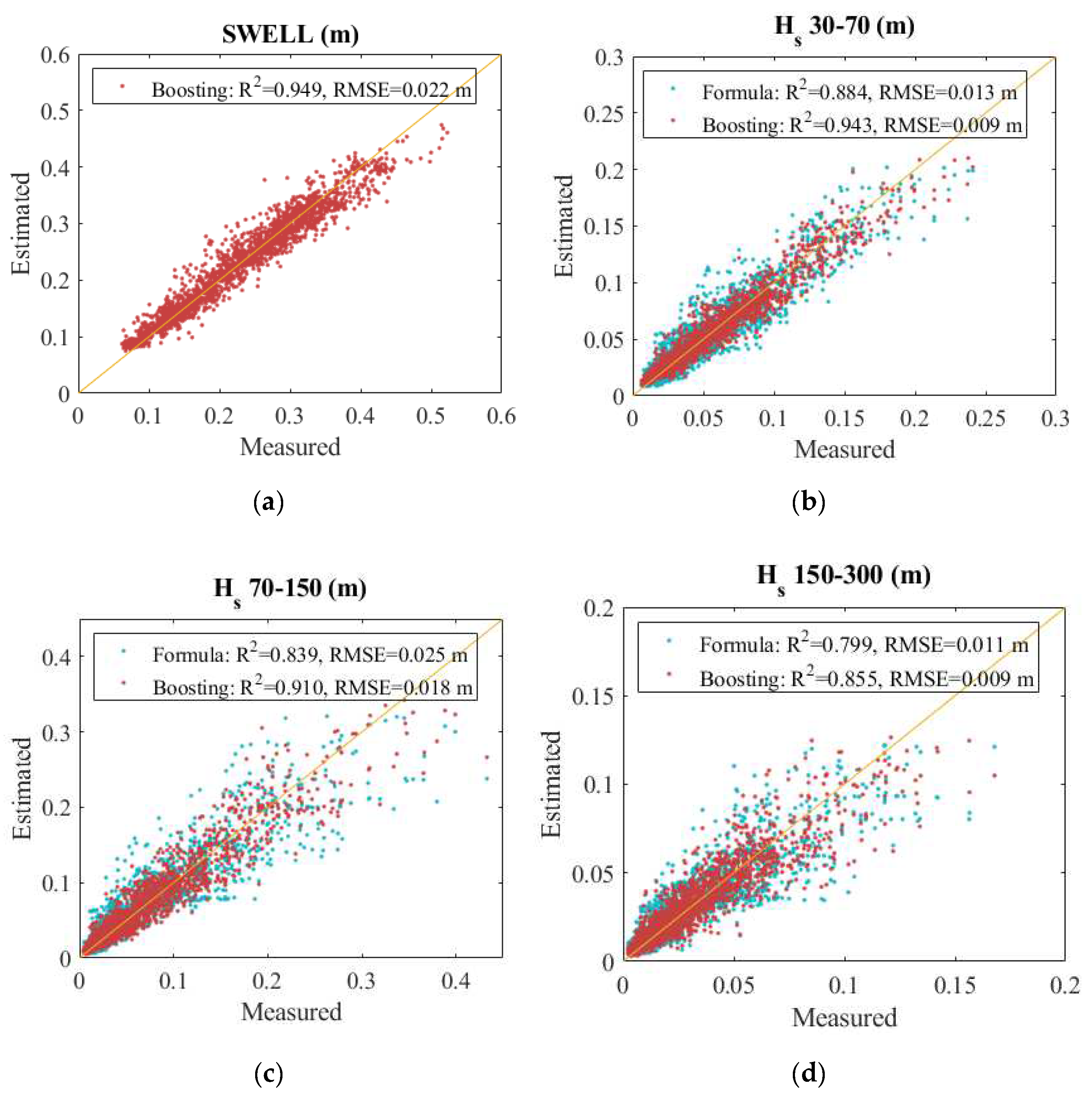
The difference between the measurement of significant wave heights, that is, those obtained through the formula and the best version of the GBM, is displayed graphically in Figure 3. The dispersion is reduced by the model, obtaining a better fitting of the diagonal. Of note is the good performance for the swell and infragravity waves in the upper frequency range (30–70 s), R2 = 0.94. As the periods increase, the efficiency worsens slightly, reducing the correlation coefficients to 0.85.
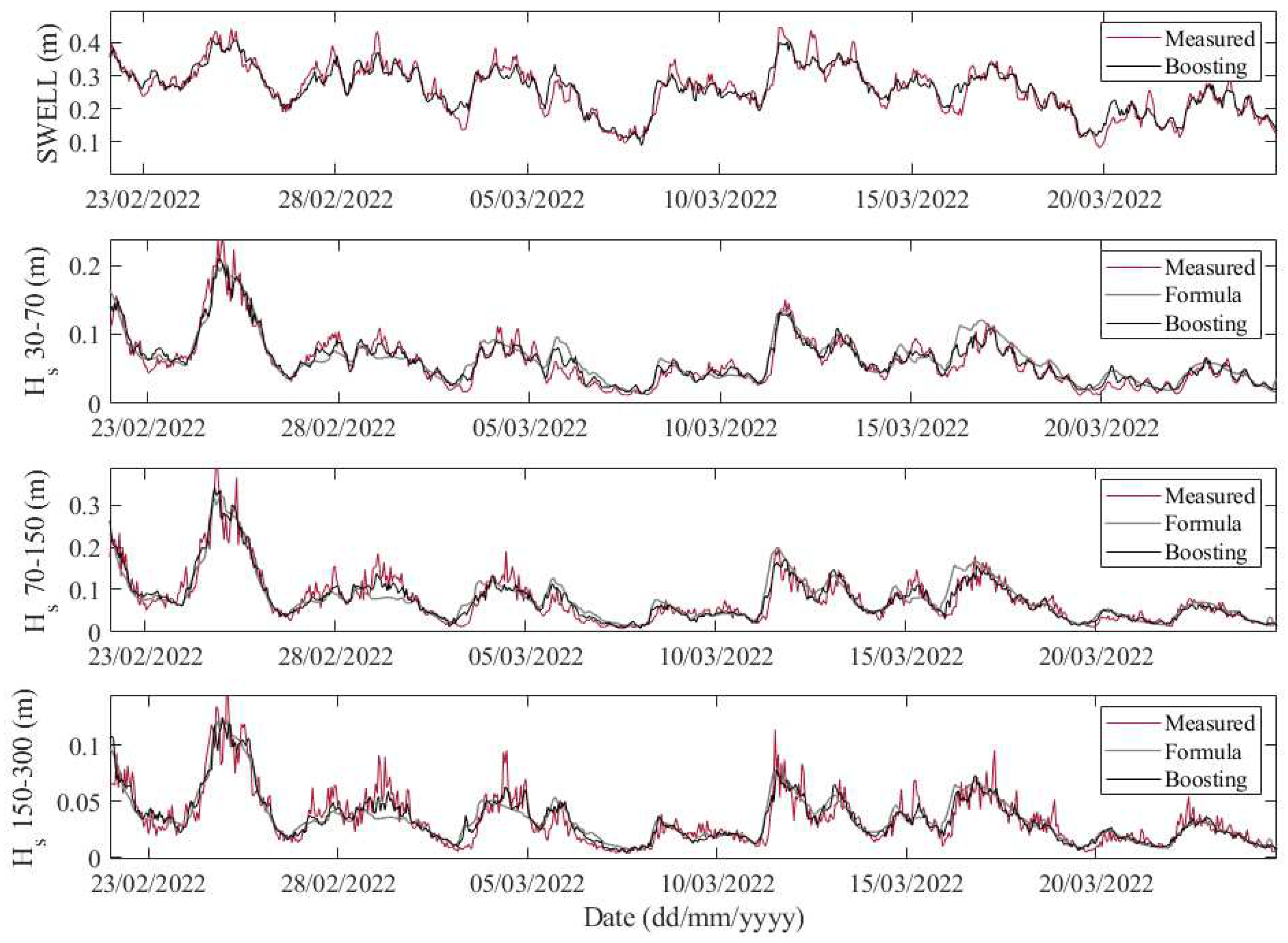
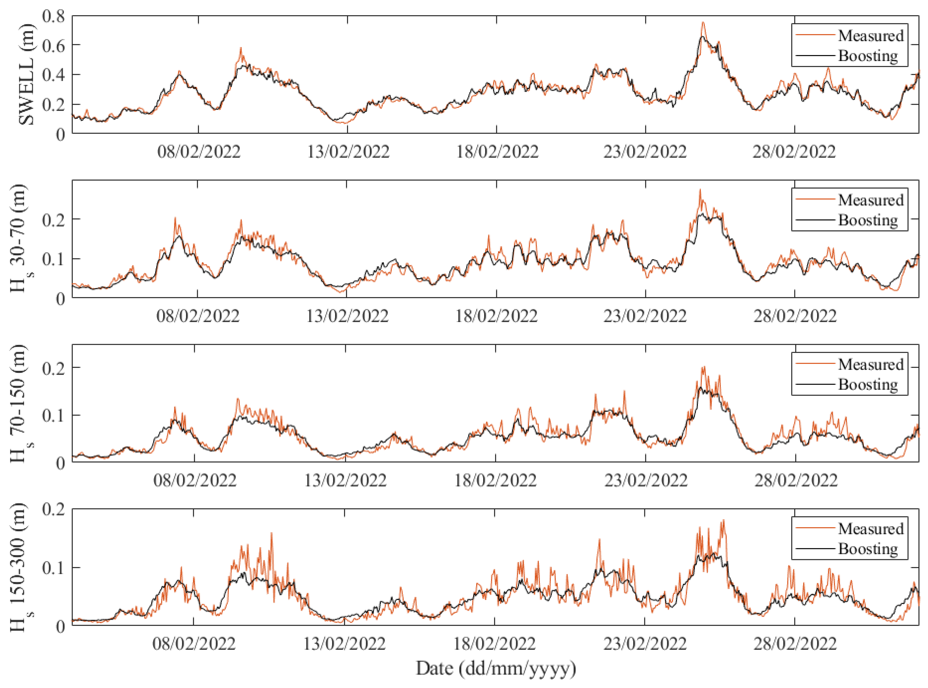
A time frame of the significant wave height as measured and estimated by the two methods discussed above is shown in Figure 4. Both predictions reflect the general trend of the real data. However, the machine-learning tool considers shorter period oscillations. This is more notable in the higher frequency band of the infragravity waves (30–70 s), where the tidal effect can be appreciated.
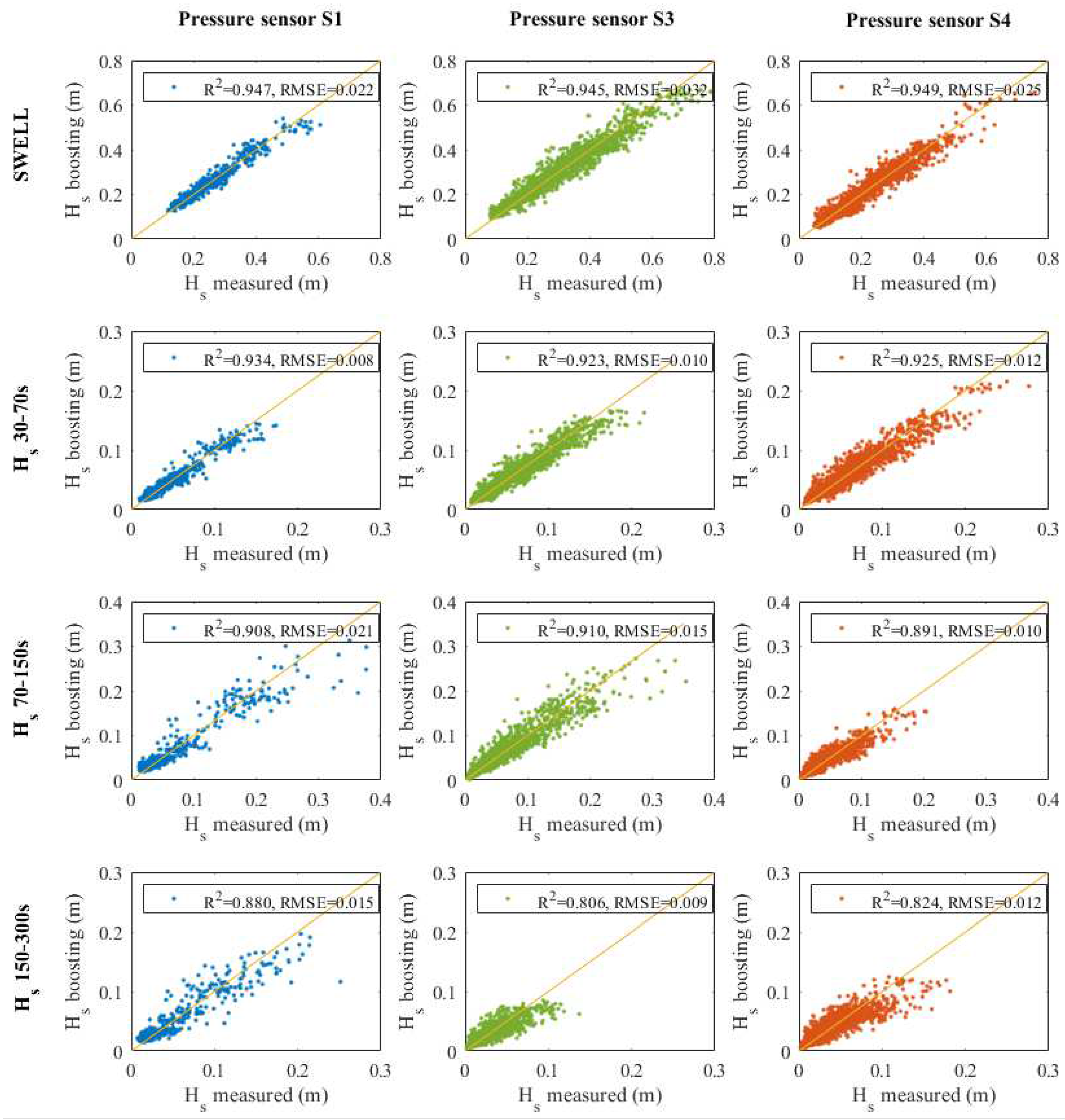
In light of these results, the gradient boosting machine was selected as the model to obtain the significant wave height in the different period ranges, using the information from the pressure sensors S1, S3 and S4 located in the berthing areas in use. The comparison between the measured and estimated Hs in the scatterplot format is shown in Figure 5. The swell presented a higher magnitude, as expected. In the case of infragravity waves, the greatest energy is centered in the 70–150 s band, in sensors S1 and S3, and in the 30–70 s range, in sensor S4. Differentiating by positions, it can be seen that the short waves vary, decreasing in the following order: S3, S4 and S1. The discrepancy between sensors S1 and S3 in terms of the long wave is not appreciable. However, S4 displays higher amplitudes in the period band 30–70 s and lower amplitudes in 70–150 s. Finally, the far infragravity waves (FIG) increase in magnitude from S3 to S4 and S1. These differences can influence ship motion and thus indicate the potential occurrence of downtimes.
In terms of prediction, the statistics used (correlation coefficient and root mean square error) report values similar to those obtained for the tide gauge. The R2 decreases with a rise in the period for all sensors. The RMSE is 2.6 cm on average for short waves, 1 cm in the 30–70 s range, 1.5 cm in the 70–150 s band, and 1.2 cm for FIG waves (150–300 s).
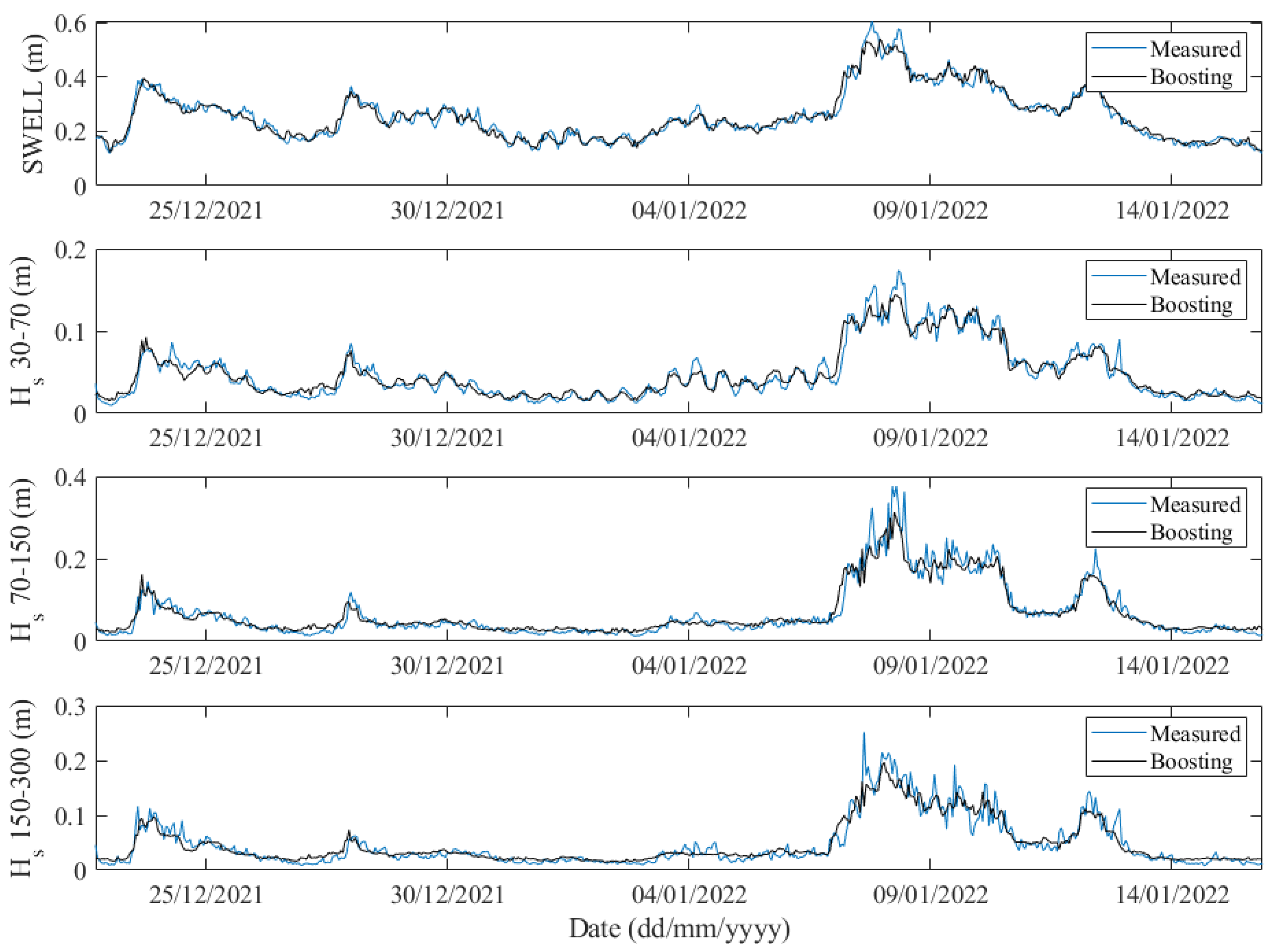
In the time records of Figure 6, Figure 7 and Figure 8, the measurement of significant wave height is compared with that obtained by the gradient boosting model in the three sensors. It is again observed how the GBM performance is more suitable for the higher frequencies. In the intervals of greatest wave energy, the measured record presents peaks that are not found in the 30–70 s and swell bands; for example, on 8 January at sensor S1, and on 10 February and 25 at sensors S3 and S4. These are the data with the greatest prediction errors, and there could be two possible causes: undetected outliers in the measured data, or incoming low frequency energy not associated with the swell and not represented through the atmospheric parameters used.
Despite these discrepancies, the models obtained managed to fit the measured waves with the appropriate accuracy for the purpose of this study. Thus, they were used as input variables for downtime forecasting with the aim of providing valuable information.

3.2. Downtime Risk Forecast

Based on the forecast met-ocean conditions at the buoy location and the prediction of significant swell and long-wave height at the berths, a model was developed to indicate the downtime risk in advance. The result was a numerical value [0–1] for each hour, this indicating the probability of problems, on the basis of which port stakeholders can make decisions about their daily operations. In order to provide recommendations on the optimal thresholds here, with safety as a priority, the performance of the model was evaluated by setting different limits and obtaining data on the number and percentages of successes and failures.
This analysis was carried out by sea state and by event. In terms of real conditions, a single event is considered to be the set of consecutive hours with real problems, regardless of the number of vessels affected. According to the model, a single event is understood as one in which the probability of downtime exceeds the cutoff point in at least two successive sea states.
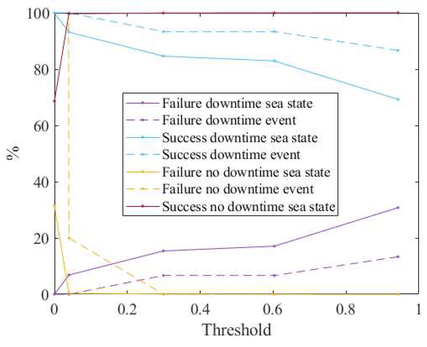
The performance of the model for each of the limits is presented in Table 4. The values set for the study vary from the minimum necessary to reach all situations (0.00048), to the maximum, which reduces failures in the incorrect identification of downtimes (false positives) to zero (0.9405). It can be observed that, with the 0.0397 threshold (3.97%), false positives affect up to 34 sea states. Discarding the hours before and after the events and the isolated data (one single sea state), only 7 h were false positives, these corresponding to three incidents. It should be noted that these correspond to a period extending over four winters. With lower thresholds, the number of false positives increases dramatically, effectively penalizing the operability of the port. With higher thresholds, one or more events are not detected, compromising port security. Therefore, the optimal threshold is considered to be 0.0397, which minimizes risks as a priority while maximizing operability.
Taking into account that there are 15 real events with downtime extending over 117 sea states and 11,228 h without problems, the percentages of success and failure in each case were obtained (Figure 9). It is worth mentioning, due to the way in which events are defined, that it is not possible to calculate them in their absence, and hence no downtime successes per event were analyzed. As expected, it was observed that as the threshold decreases, undetected incidents are lower (purple lines), and therefore the number of successes increases (blue lines). The consequence of this is that the behavior of the model for the cases without problems worsens, thus penalizing the operability of the port. The potentiality of the model lies at the point where failures are minimized and successes are maximized, which was considered to be the threshold 0.0397 (3.97%), in which safety was prioritized. With this value, the sea state forecast has an accuracy rate of 99.7% when there are no problems and a rate of 93% in the case of downtime.
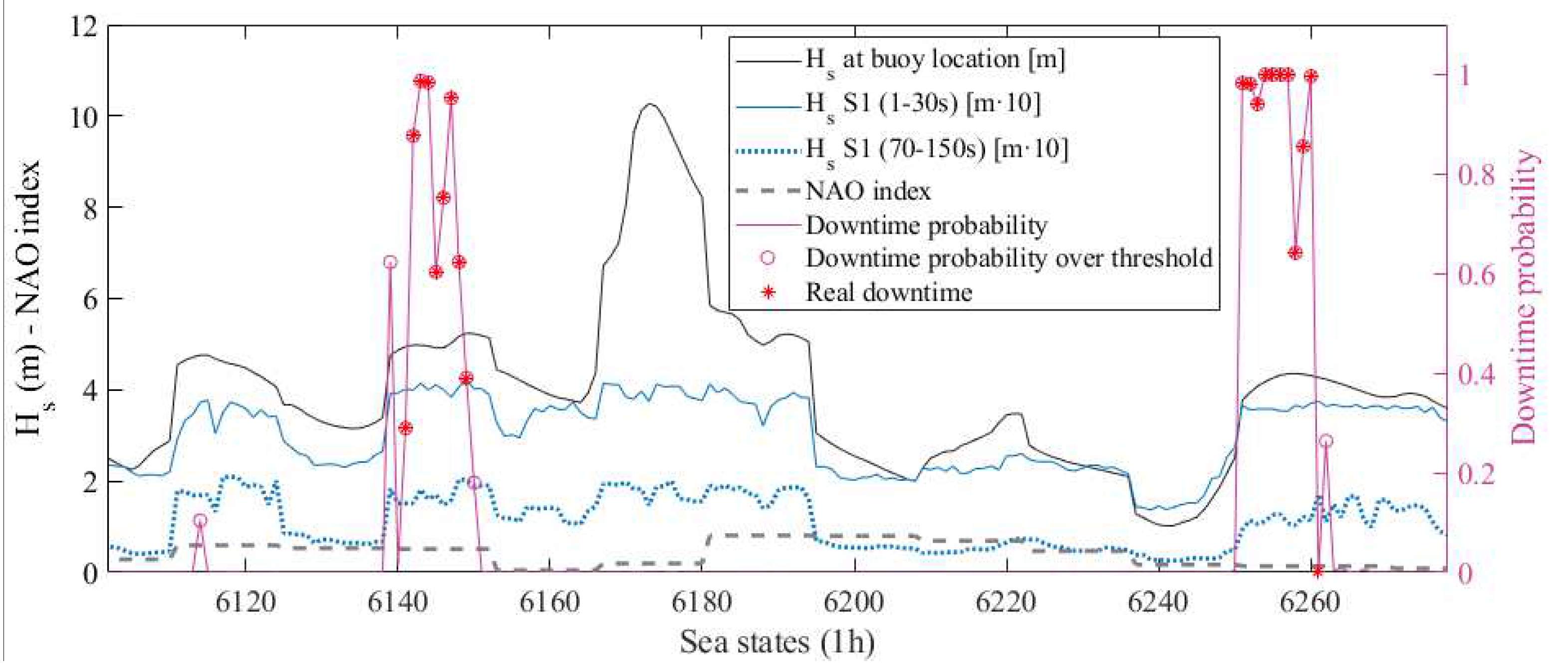
With the threshold established, the time series was analyzed representing the downtime probability, NAO index, significant wave heights at the buoy location, and at sensor S1 (Figure 10). In this figure, the isolated data (sea state 6114), false negatives linked to an event (time 6261) and false positives associated with events (sea state 6139, 6150 and 6262) can be identified. In this time window there were no undetected events. It should be noted that the closer the output of the model is to 1, the greater the probability of problems, and thus the chance of a false positive occurring is reduced.
Regarding the met-ocean parameters, those addressed were considered because of the high influence of wave height as demonstrated in the literature, together with the novelty of using the weather index. It can be observed how in the two events (set of hours with real downtime) of the frame, the NAO is positive, as is the case in the remaining 13 events. Moreover, as expected, the problems occurred with high wave heights. Additionally, these circumstances can arise but might not result in downtime, as was the case between sea states 6167 and 6180.
These hours are from 14 November 2019, when the significant wave height reached 10.12 m at the buoy. The agitation in the basin was similar to that predicted for the period of the two downtime events. However, image and video evidence was available here, and showed that a 229 m vessel, the Majestic Sky, was unloading (Figure 11) at the time. Although it did not have the gangway in place (as can be seen in the right-hand photo in Figure 11), operations continued and the ship remained at berth.
The results of this section have illustrated the high performance of the model, which is optimized when applied as it is proposed: a downtime alert is given when the probability exceeds 3.9% in two consecutive sea states. Thus, its behavior is optimal both in the detection of problems, guaranteeing the safety of port operations and the people involved, and in the adequate assessment of downtime risks, even in extreme circumstances, thus maximizing the port’s operation.

4. Conclusions

This study presents a decision-making tool for port operations based on real downtimes identified in the Outer Port of Punta Langosteira (A Coruña, Spain). For this purpose, a combination of sea oscillations measured at four berth locations, and a machine-learning method for short- and long-wave prediction, was used. The results of this, together with the met-ocean forecast conditions, allowed the development of a classification model in which the output is an accurate prediction of the probability of downtime for each sea state.
The application of the regression model in the prediction of significant wave height in the tide gauge increased the correlation coefficient with respect to the empirical formulation. The high correlation found shows that the long wave that is present depends fundamentally on the swell, and is therefore a bound wave.
When wave direction is added to the model, the correlation increases by 4%. Moreover, the use of atmospheric parameters (wind speed and direction, and NAO index) leads to an increase in the fitting of an additional 2.5%. Thus, the application of the proposed methodology achieved an improvement in the correlation coefficient of 6% and a reduction in the RMSE of 0.004 m (26.5%) for infragravity waves with respect to the existing formulation.
The methodology tested with the tide gauge was applied to the data measured by three pressure sensors located in the mooring areas, obtaining a R2 of approximately 0.95 for the swell and 0.93 for the infragravity waves of the 30–70 s range. Furthermore, the errors were 3.7% and 4%, respectively.
Another relevant novelty presented in this paper is that, based on the forecast of downtime probability, the behavior of the model was studied at different cutoff points. It was concluded that two consecutive sea states exceeding the threshold of 3.97% is the limit that renders the forecast adequate for minimizing risks and maximizing operations, thus prioritizing safety. In terms of sea states, the success ratio reaches 93% and 99.7% for downtime detection and absence of problems, respectively. Looking at the events, three false positives were detected in five years, and zero situations were overlooked. Therefore, by using the tool as proposed, eliminating the risk of operational and safety problems would have come at a cost of just 0.6 unnecessary interruptions of operations per year.
In summary, the tool is directly applicable at the study port with the forecast weather variables as input and will support in operational decision-making based on the risk stakeholders want to assume. It can also be enhanced by extending the database for both downtime and weather variables or by including new variables such as the period of infragravity movements of ships. Nevertheless, this study presents an accessible and exportable method for downtime forecasting, including innovative variables, which can be used as a reference model in risk control and optimization of port operations.

Author Contributions

Conceptualization, R.C. and H.C.; methodology, R.C. and H.C.; software, H.C.; validation, H.C. and R.C.; formal analysis, R.C.; investigation, R.C.; resources, R.C., H.C. and A.F.; data curation, R.C.; writing—original draft preparation, R.C.; writing—review and editing, R.C., A.F. and E.P.; visualization, R.C.; project administration, A.F., J.S. and E.P.; funding acquisition, A.F., J.S. and E.P. All authors have read and agreed to the published version of the manuscript.

Funding

This research was carried out with the grant PID2020-112794RB-I00 funded by MCIN/AEI/10.13039/501100011033 and the FPI predoctoral grants from the Spanish Ministry of Science, Innovation, and Universities (PRE2018-083777 and PRE2021-100141).

Institutional Review Board Statement

Not applicable.

Informed Consent Statement

Not applicable.

Data Availability Statement

Data available on request due to privacy restrictions.

Acknowledgments

The authors are grateful to the Port Authority of A Coruña (Spain), Andrés Guerra and Juan Diego Pérez in particular, and the crews of the referenced vessels for their kind collaboration.

Conflicts of Interest

The authors declare no conflict of interest.

References

  1. van Deyzen, A.F.J.; Beimers, P.B.; van Der Lem, J.C.; Messiter, D.; De Bont, J.A.M. To Improve the Efficiency of Ports Exposed to Swell. In Proceedings of the Australasian Coasts & Ports Conference 2015: 22nd Australasian Coastal and Ocean Engineering Conference and the 15th Australasian Port and Harbour Conference, Auckland, New Zealand, 15–18 September 2015; pp. 919–926. [Google Scholar]
  2. McComb, P.; Zyngfogel, R.; Gomez, B.P. Predicting Infragravity Waves in Harbours—An Evaluation of Published Equations and Their Use in Forecasting Operational Thresholds. Coast. Eng. Proc. 2020, 36, 7. [Google Scholar] [CrossRef]
  3. Sun, J.; Wang, H.; Chen, J. Decision-Making of Port Enterprise Safety Investment Based on System Dynamics. Processes 2020, 8, 1235. [Google Scholar] [CrossRef]
  4. Kadir, Z.A.; Mohammad, R.; Othman, N.; Amrin, A.; Muhtazaruddin, M.N.; Abu-Bakar, S.H.; Muham, F. Risk Management Framework for Handling and Storage of Cargo at Major Ports in Malaysia towards Port Sustainability. Sustainability 2020, 12, 516. [Google Scholar] [CrossRef] [Green Version]
  5. Rosa-Santos, P.J.; Taveira-Pinto, F. Experimental Study of Solutions to Reduce Downtime Problems in Ocean Facing Ports: The Port of Leixões, Portugal, Case Study. J. Appl. Water Eng. Res. 2013, 1, 80–90. [Google Scholar] [CrossRef]
  6. Spanish Port Authority ROM 3.1-99. Planning, Management and Operation in Port Areas. In Project of the Maritime Configuration of Ports; Access Channels and Floating Areas: Madrid, Spain, 2000; Volume 3, ISBN 9788578110796. [Google Scholar]
  7. Thoresen, C.A. Port Designer’S Handbook: Recommendations and Guidelines; Thomas Telford Publishing: London, UK, 2003; ISBN 0727732242. [Google Scholar]
  8. PIANC Criteria for Movements of Moored Ships in Harbours—A Practical Guide; MarCom Working Group: Brussels, Belgium, 1995; ISBN 2-87223-070-X.
  9. Spanish Port Authority ROM 2.0-11. Design and Construction of Berthing & Mooring Structures. In Recommendations for the Design and Execution of Berthing and Mooring Works; V.A. Impresores: Madrid, Spain, 2011; ISBN 9788488975409. [Google Scholar]
  10. Prpić-Orsić, J.; Slapnicar, V.; Turk, A. Berth Operability Estimation Related to Ship Motion. Trans. Famena 2014, 38, 13–24. [Google Scholar]
  11. Kwak, M.S.; Moon, Y.H.; Pyun, C.K. A Study on Analysis of Moored Ship Motion Considering Harbor Resonance. J. Korean Soc. Civ. Eng. 2013, 33, 595–608. [Google Scholar] [CrossRef] [Green Version]
  12. Figuero, A.; Sande, J.; Peña, E.; Alvarellos, A.; Rabuñal, J.R.; Maciñeira, E. Operational Thresholds of Moored Ships at the Oil Terminal of Inner Port of A Coruña (Spain). Ocean Eng. 2019, 172, 599–613. [Google Scholar] [CrossRef]
  13. Alvarellos, A.; Figuero, A.; Carro, H.; Costas, R.; Sande, J.; Guerra, A.; Peña, E.; Rabuñal, J. Machine Learning Based Moored Ship Movement Prediction. J. Mar. Sci. Eng. 2021, 9, 800. [Google Scholar] [CrossRef]
  14. Romano-Moreno, E.; Tomás, A.; Diaz-Hernandez, G.; Lara, J.L.; Molina, R.; García-Valdecasas, J. A Semi-Supervised Machine Learning Model to Forecast Movements of Moored Vessels. J. Mar. Sci. Eng. 2022, 10, 1125. [Google Scholar] [CrossRef]
  15. López, I.; López, M.; Iglesias, G. Artificial Neural Networks Applied to Port Operability Assessment. Ocean Eng. 2015, 109, 298–308. [Google Scholar] [CrossRef]
  16. Troch, C.; Terblanche, L.; Rossouw, M.; Ntantala, Z.; du Plessis, G. Long-Wave Mitigation Study for the Port of Ngqura. In Proceedings of the Coastal Engineering, Online, 6–9 October 2020; p. 14. [Google Scholar]
  17. Scott, D.; Taylor, D.; El-Solh, S.; Elliott, T. Port Simulation Modelling and Economic Assessment. J. Mar. Sci. Eng. 2016, 4, 16. [Google Scholar] [CrossRef] [Green Version]
  18. Gómez, R.; Molina, R.; Camarero, A.; de los Santos, F. Development of a Terminal Operability Forecasting System: Analysis of the Effects That Wind Generates over Vessel Performance. Coast. Eng. 2014, 34, 16. [Google Scholar] [CrossRef]
  19. Campos, Á.; García-Valdecasas, J.M.; Molina, R.; Castillo, C.; Álvarez-Fanjul, E.; Staneva, J. Addressing Long-Term Operational Risk Management in Port Docks under Climate Change Scenarios-A Spanish Case Study. Water 2019, 11, 2153. [Google Scholar] [CrossRef] [Green Version]
  20. Camus, P.; Tomás, A.; Díaz-Hernández, G.; Rodríguez, B.; Izaguirre, C.; Losada, I.J. Probabilistic Assessment of Port Operation Downtimes under Climate Change. Coast. Eng. 2019, 147, 12–24. [Google Scholar] [CrossRef]
  21. Izaguirre, C.; Losada, I.J.; Camus, P.; Vigh, J.L.; Stenek, V. Climate Change Risk to Global Port Operations. Nat. Clim. Chang. 2021, 11, 14–20. [Google Scholar] [CrossRef]
  22. Jebbad, R.; Sierra, J.P.; Mösso, C.; Mestres, M.; Sánchez-Arcilla, A. Assessment of Harbour Inoperability and Adaptation Cost Due to Sea Level Rise. Application to the Port of Tangier-Med (Morocco). Appl. Geogr. 2022, 138, 102623. [Google Scholar] [CrossRef]
  23. Sierra, J.P.; Genius, A.; Lionello, P.; Mestres, M.; Mösso, C.; Marzo, L. Modelling the Impact of Climate Change on Harbour Operability: The Barcelona Port Case Study. Ocean Eng. 2017, 141, 64–78. [Google Scholar] [CrossRef] [Green Version]
  24. Molina-Sanchez, R.; Campos, Á.; de Alfonso, M.; de los Santos, F.J.; Rodríguez-Rubio, P.; Pérez-Rubio, S.; Camarero-Orive, A.; Álvarez-Fanjul, E. Assessing Operability on Berthed Ships. Common Approaches, Present and Future Lines. J. Mar. Sci. Eng. 2020, 8, 255. [Google Scholar] [CrossRef] [Green Version]
  25. Dong, G.; Yan, M.; Zheng, Z.; Ma, X.; Sun, Z.; Gao, J. Experimental Investigation on the Hydrodynamic Response of a Moored Ship to Low-Frequency Harbor Oscillations. Ocean Eng. 2022, 262, 112261. [Google Scholar] [CrossRef]
  26. Costas, R.; Figuero, A.; Peña, E.; Sande, J.; Rosa-santos, P. Integrated Approach to Assess Resonance between Basin Eigenmodes and Moored Ship Motions with Wavelet Transform Analysis and Proposal of Operational Thresholds. Ocean Eng. 2022, 247, 110678. [Google Scholar] [CrossRef]
  27. Thiebaut, S.; McComb, P.; Vennell, R. Prediction of Coastal Far Infragravity Waves from Sea-Swell Spectra. J. Waterw. Port Coastal Ocean Eng. 2013, 139, 34–44. [Google Scholar] [CrossRef]
  28. Costas, R.; Figuero, A.; Sande, J.; Peña, E.; Guerra, A. The Influence of Infragravity Waves, Wind, and Basin Resonance on Vessel Movements and Related Downtime at the Outer Port of Punta Langosteira, Spain. Appl. Ocean Res. 2022, 129, 103370. [Google Scholar] [CrossRef]
  29. Wang, C.-N.; Yang, F.-C.; Vo, N.T.M.; Nguyen, V.T.T. Wireless Communications for Data Security: Efficiency Assessment of Cybersecurity Industry—A Promising Application for UAVs. Drones 2022, 6, 363. [Google Scholar] [CrossRef]
  30. Nguyen, N.A.T.; Wang, C.N.; Dang, L.T.H.; Dang, L.T.T.; Dang, T.T. Selection of Cold Chain Logistics Service Providers Based on a Grey AHP and Grey COPRAS Framework: A Case Study in Vietnam. Axioms 2022, 11, 154. [Google Scholar] [CrossRef]
  31. Wiegel, M.; de Boer, W.; van Koningsveld, M.; van der Hout, A.; Reniers, A. Global Mapping of Seaport Operability Risk Indicators Using Open-Source Metocean Data. J. Mar. Sci. Eng. 2021, 9, 695. [Google Scholar] [CrossRef]
  32. Puertos Del Estado (Spanish Port Authority). Available online: http://www.puertos.es/es-es/oceanografia/Paginas/portus.aspx (accessed on 23 October 2020).
  33. Gao, J.; Ji, C.; Liu, Y.; Ma, X.; Gaidai, O. Influence of Offshore Topography on the Amplification of Infragravity Oscillations within a Harbor. Appl. Ocean Res. 2017, 65, 129–141. [Google Scholar] [CrossRef]
  34. Bertin, X.; de Bakker, A.; van Dongeren, A.; Coco, G.; André, G.; Ardhuin, F.; Bonneton, P.; Bouchette, F.; Castelle, B.; Crawford, W.C.; et al. Infragravity Waves: From Driving Mechanisms to Impacts. Earth-Sci. Rev. 2018, 177, 774–799. [Google Scholar] [CrossRef] [Green Version]
  35. Gao, J.; Ma, X.; Dong, G.; Chen, H.; Liu, Q.; Zang, J. Investigation on the Effects of Bragg Reflection on Harbor Oscillations. Coast. Eng. 2021, 170, 103977. [Google Scholar] [CrossRef]
  36. Seetharam, K.; Lerose, A.; Fazio, R.; Marino, J. Dynamical Scaling of Correlations Generated by Short- and Long-Range Dissipation. Phys. Rev. B 2022, 105, 184305. [Google Scholar] [CrossRef]
  37. Niu, X. Conditions for the Occurrence of Notable Edge Waves Due to Atmospheric Disturbances. Appl. Ocean Res. 2020, 101, 102255. [Google Scholar] [CrossRef]
  38. Sun, Q.; Niu, X. Harbor Resonance Triggered by Atmospherically Driven Edge Waves. Ocean Eng. 2021, 224, 108735. [Google Scholar] [CrossRef]
  39. Ayet, A.; Chapron, B. The Dynamical Coupling of Wind-Waves and Atmospheric Turbulence: A Review of Theoretical and Phenomenological Models. Boundary-Layer Meteorol. 2022, 183, 1–33. [Google Scholar] [CrossRef]
  40. Gao, J.; Ji, C.; Gaidai, O.; Liu, Y.; Ma, X. Numerical Investigation of Transient Harbor Oscillations Induced by N-Waves. Coast. Eng. 2017, 125, 119–131. [Google Scholar] [CrossRef]
  41. Gao, J.; Ma, X.; Zang, J.; Dong, G.; Ma, X.; Zhu, Y.; Zhou, L. Numerical Investigation of Harbor Oscillations Induced by Focused Transient Wave Groups. Coast. Eng. 2020, 158, 103670. [Google Scholar] [CrossRef]
  42. Hilton, D.; Davidson, M.; Scott, T. Seasonal Predictions of Shoreline Change, Informed by Climate Indices. J. Mar. Sci. Eng. 2020, 8, 616. [Google Scholar] [CrossRef]
  43. Wiggins, M.; Scott, T.; Masselink, G.; McCarroll, R.J.; Russell, P. Predicting Beach Rotation Using Multiple Atmospheric Indices. Mar. Geol. 2020, 426, 106207. [Google Scholar] [CrossRef]
  44. Scott, T.; McCarroll, R.J.; Masselink, G.; Castelle, B.; Dodet, G.; Saulter, A.; Scaife, A.A.; Dunstone, N. Role of Atmospheric Indices in Describing Inshore Directional Wave Climate in the United Kingdom and Ireland. Earth’s Futur. 2021, 9, e2020EF001625. [Google Scholar] [CrossRef] [PubMed]
  45. Lorente, P.; Basañez Mercader, A.; Piedracoba, S.; Pérez-Muñuzuri, V.; Montero, P.; Sotillo, M.G.; Álvarez-Fanjul, E. Long-Term Skill Assessment of SeaSonde Radar-Derived Wave Parameters in the Galician Coast (NW Spain). Int. J. Remote Sens. 2019, 40, 9208–9236. [Google Scholar] [CrossRef]
  46. Hurrell, J.W. Decadal Trends in the North Atlantic Oscillation: Regional Temperatures and Precipitation. Science 1995, 269, 676–679. [Google Scholar] [CrossRef] [PubMed] [Green Version]
  47. Nelson, R.C.; Treloar, P.D.; Lawson, N.V. The Dependency of Inshore Long Waves on the Characteristics of Offshore Short Waves. Coast. Eng. 1988, 12, 213–231. [Google Scholar] [CrossRef]
  48. Bowers, E.C. Low Frequency Waves in Intermediate Water Depths. In Proceedings of the 23rd International Conference on Coastal Engineering, Venice, Italy, 4–9 October 1992; p. 252. [Google Scholar]
  49. Lara, J.L.; Martin, F.L.; Losada, I.J.; Díaz, G. Experimental Analysis of Long Waves At Harbour Entrances. In Proceedings of the Coastal Engineering Conference, Lisbon, Portugal, 19–24 September 2004; pp. 1308–1320. [Google Scholar]
  50. Gracia, S.; Olivito, J.; Resano, J.; Martin-del-Brio, B.; de Alfonso, M.; Álvarez, E. Improving Accuracy on Wave Height Estimation through Machine Learning Techniques. Ocean Eng. 2021, 236, 108699. [Google Scholar] [CrossRef]
  51. Friedman, J.H. Greedy Function Approximation: A Gradient Boosting Machine. Ann. Stat. 2001, 429, 1189–1232. [Google Scholar] [CrossRef]
  52. Natekin, A.; Knoll, A. Gradient Boosting Machines, a Tutorial. Front. Neurorobot. 2013, 7, 21. [Google Scholar] [CrossRef] [PubMed] [Green Version]
  53. Hastie, T.; Tibshirani, R.; Friedman, J.H. The Elements of Statistical Learning; Springer: New York, NY, USA, 2001. [Google Scholar]
  54. López, M.; Iglesias, G.; Kobayashi, N. Long Period Oscillations and Tidal Level in the Port of Ferrol. Appl. Ocean Res. 2012, 38, 126–134. [Google Scholar] [CrossRef]
  55. Guerrini, M.; Bellotti, G.; Fan, Y.; Franco, L. Numerical Modelling of Long Waves Amplification at Marina Di Carrara Harbour. Appl. Ocean Res. 2014, 48, 322–330. [Google Scholar] [CrossRef]
Figure 1. (a) Spain, showing the location of A Coruña, (b) situation of the port, buoy and zoom for section c, (c) plan view of the Outer Port of Punta Langosteira and position of pressure sensors (S1, S2, S3, S4, S5 and S6) and the tide gauge.
Jmse 11 00536 g001
Figure 2. Flowchart of the proposed method to estimate downtime probability.
Jmse 11 00536 g002
Figure 3. Scatterplot of Hs measured and estimated through the classical formula (blue) and the GBM (maroon) with met-ocean parameters for (a) Hs swell, (b) Hs 30–70 s, (c) Hs 70–150 s and (d) Hs 150–300 s.
Jmse 11 00536 g003
Figure 4. Measured data (maroon) and forecast data with the formula (grey) and with GBM (black) of the Hs at the tide gauge for the different frequency ranges.
Jmse 11 00536 g004
Figure 5. Scatterplots of the data measured by sensors S1 (blue), S3 (green) and S4 (orange) and their prediction with the model in the different frequency bands.
Jmse 11 00536 g005
Figure 6. Measured and predicted data with the formula and with GBM of the Hs in sensor S1 for the different frequency ranges.
Jmse 11 00536 g006
Figure 7. Measured and predicted data with the formula and with GBM of the Hs in sensor S3 for the different frequency ranges.
Jmse 11 00536 g007
Figure 8. Measured and predicted data with the formula and with GBM of the Hs in sensor S4 for the different frequency ranges.
Jmse 11 00536 g008
Figure 9. Relationship between different thresholds and model performance: successes and failures for sea states and events.
Jmse 11 00536 g009
Figure 10. Time series of significant wave heights, NAO index, and downtime probability with real events.
Jmse 11 00536 g010
Figure 11. (a,b) The vessel Majestic Sky in operations on 14 November 2019 at 12 h (sea state 6172 from Figure 10).
Jmse 11 00536 g011
Table 1. Vessel characteristics, berthing area, date, and details of downtime events.
NameDWT (t)Overall Length (m)Beam (m)TypeLocation at DockDate
Lowlands Saguenay37,152180.030.0OperabilityZ52 February 2017
Isartal371187.812.9OperabilityZ530 January 2019
Manisa Alena35,063108.030.0OperabilityZ511 November 2019
Wilson Newport8321123.016.7OperabilityZ520 November 2019
Juergen K378588.812.5OperabilityZ313 February 202
Waaldijk489189.914.4OperabilityZ416 February 202
Amalia35,063180.030.0OperabilityZ620 November 2019
Waaldijk489189.914.4OperabilityZ629 October 2020
John Paul K424790.315.2SafetyZ42 February2017
Fulda443399.912.8SafetyZ52 February 2017
Moraime7300118.016.5SafetyZ317 January 2018
Zealand Beatrix13,089134.720.5SafetyZ412 November 2019
Rose3603101.114.6SafetyZ320 November 2019
Juergen K378588.812.5SafetyZ413 February 2020
Mario C13,000130.022.0SafetyZ528 October 2020
Table 2. Coefficients k, α, β and γ obtained from the fitting to the classical formula, and comparison with those of other authors.
Authorskαβγ
Port of Langosteira Hs 30–70 s0.000421.3740.536−0.566
Port of Langosteira Hs 70–150 s0.000171.6640.815−0.571
Port of Langosteira Hs 150–300 s12.3431.4740.7612.698
Ref. [54], Port of Ferrol0.0051.2651.30.328
Ref. [54], Port of Ferrol0.0021.2641.293-
Ref. [48], Port Talbot0.00641.321.170.34
Ref. [48], Shoreham Port0.00740.930.990.06
Ref. [48], Barrow-in-Furness0.00241.081.590.36
Ref. [55], Marina di Carrara0.00841.20.780
Table 3. Statistical comparison of forecast methods and input parameters for significant wave heights at the tide gauge.
MethodFormulaGradient Boosting (GBM)
Input ParametersHs, Tp and SWLHs, Tp and SWLHs, Tp, Dir and SWLHs, Tp, Dir, SWL, Vw, Dirw and NAO
StatisticsR2RMSE (m)R2RMSE (m)R2RMSE (m)R2RMSE (m)
Hs swell (1–30 s)--0.880.0330.930.0260.950.022
Hs LIG (30–70 s)0.880.0130.900.0120.920.0110.940.009
Hs UPG (70–150 s)0.840.0250.850.0240.880.0210.910.018
Hs FIG (150–300 s)0.800.0110.800.0110.830.0100.860.009
Table 4. Confusion matrix data with different thresholds for sea states (1 h) and events (at least 2 consecutive hours).
ThresholdSea StateEvent
DowntimeNo DowntimeDowntimeNo Downtime
SuccessFailuresSuccessFailuresSuccessFailuresFailures
0.940529813611,22801320
0.603581972011,22531410
0.298837991811,21991410
0.039730109811,194341503
0.000048117077063522150501
Disclaimer/Publisher’s Note: The statements, opinions and data contained in all publications are solely those of the individual author(s) and contributor(s) and not of MDPI and/or the editor(s). MDPI and/or the editor(s) disclaim responsibility for any injury to people or property resulting from any ideas, methods, instructions or products referred to in the content.