Article

The Hydrostatic Buckling of SPM Systems of Fish Cages and a Design Method to Prevent It

The Faculty of Mechanical Engineering, Technion–Israel Institute of Technology, Haifa 32000, Israel
*
Author to whom correspondence should be addressed.
J. Mar. Sci. Eng. 2023, 11(3), 538; https://doi.org/10.3390/jmse11030538
Submission received: 28 January 2023 / Revised: 25 February 2023 / Accepted: 28 February 2023 / Published: 2 March 2023

Abstract

:
This study presents an inherent buckling issue of SPM (Single Point Mooring) systems for open sea aquaculture and a design method to analyze and solve this issue. The SPM arrangement of a row of cages is very efficient, as it minimizes the anchoring load by masking of the current applied to the downstream cages, hence saves anchors and mooring lines. However, a sudden reversal of the current direction presents a risk of buckling of the row of cages, if it applies a compression load along the array of cages before rotation of the entire cage system takes place. This study presents the concept of Hydrostatic Buckling of a row of cages and a method of design and analysis to control the stability of the system at the situation of sudden current reversal. First, a simple method for preliminarily assessment by applying the principle of virtual work is formulated. Then, an analysis of the structure by a parametric finite elements code is presented. The reversal current limits for the stability of the structure, are parametrically studied, by the analyses of two hypothetical practical scenarios. This study presents practical design tools and results, such as the method of the analysis, simplified loading states for representing the critical events, the scantlings of the structure, as well as guidelines for designing a SPM system of cages that withstand critical situations of reversal current.

1. Introduction

Given that overfishing in the oceans is continuously increasing, humans need alternative sources for seafood to feed the planet’s ever-growing population. With an anticipated 10 billion people expected to inhabit the planet by 2050, the demand for animal protein will increase by 52 percent [1]. Sustainable and healthy approaches to feed the world population are more critical than ever before and the role of Aquaculture is of utmost importance. Due to climate changes, overexploitation of stocks of wild fish and many more factors, there are strong doubts whether the production of wild–caught fish will increase [2], even though the production of wild–caught fish was not decreased nor increased in the past 30 years [3]. Hence, many, such as Shainee et al. [4], propose to enhance the aquaculture sector.
It has been suggested to move the farming of fish further offshore [5,6], but strong currents and high waves set difficulties. Moving to open sea requires new designs for fish farms that are operable under extreme environmental loads. Yu et al. [7] presented an inspiring idea of using ship aquaculture platforms to expand offshore farming, which require large capital and further research. Lader et al. [8] presented an experimental study of wave loads applied to net panels and suggested that, to reduce loads, complaint structures are required. Dong et al. [9] conducted a series of parametric studies on drag force and deformation of the elastic net cage using a numerical simulation model. The design for offshore fish farms must both keeps the volume of the cages and minimizes the high loads. The complaint structures, which efficiently reduce the wave loads and the structural stresses, are sensitive to buckling while subjected to varying conditions of waves and currents.
Researchers and designers proposed several concepts for open sea cages. For example, Shainee et al. [10] presented a self-submersible SPM (Single Point Mooring) cage of a sphere-like polygon shape and showed, by numerical investigation, its effective function at the environment of high waves. Liu et al. [11] preformed a numerical study on the mooring forces developed on an integrated fish cage array. Drimer [12] introduced the SUBFLEX SPM system, designed to a maximum wave height of 17 m, and presented its design principles. Several open sea aquaculture companies operated the SUBFLEX systems in offshore Israel since 2006. Milich and Drimer [13] proposed a larger and improved SUBFLEX SPM system, analyzed it and specified its scantlings. The “Open-Sea” company successfully operated this system offshore Israel from 2017 to 2022 with no failures.
The SPM system has several advantages over the traditional grid array of cages with multiple anchors. The main advantage, as presented by DeCew et al. [14], is the ability to align with the current or weather direction, minimizing the projected area, thus decreasing the environmental loads and the load effects in the structure. There is also a probable reduction of the mooring costs per cage. The issue of volume keeping in the net cages was solved, for the SPM cage system, by integrating a rigid Front Frame between the SPM and the cages [12]. The arrangement, connections, and mooring, of open sea cages systems, play a significant role in resisting the environmental loads (waves, current) applied to the system, while keeping functional space for the fishes. The increase of water depth, somehow reduces the efficiency of the SPM system, as it requires a longer mooring main line, which increases the circular area occupied by the system around the anchoring point on the seabed. An environmental benefit however, is the increase of the distribution area of fish waste.
An inherent drawback of the SPM system of fish cages arranged in a row connected by ropes is the practically zero structural rigidity to loads applied from the aft toward the anchor. Although such loads may cause sever operational failures as loose of volume and hence fishes, we found no literature that address this issue. The objective of this study is to develop and formulate a method to assess possible collapse of a row of cages integrated to a SPM open sea aquaculture system and to address the design of a system that is not likely to buckle at the expected sea conditions.
This article presents a new concept of buckling of a row of cages, which we term Hydrostatic Buckling, as the critical load to initiate it depends on the hydrostatic stability of the cages. Than a new method to analyze and control the stability of the system at the situation of sudden current reversal is developed. Following the formulation and verification of the method a parametric study demonstrates the effect of the design parameters on the critical opposing current that will initiate buckling. The study provides guidelines for designing a SPM system of cages that withstand critical situations of reversal current.
Following this introduction, Section 2 specifies the design principles and the parameters, of the SPM aquaculture system that we present as an example. Section 3 presents our simplified method to assess the stability at opposing current. Section 4 presents the procedure of analyzing a multi-cage system. Section 5 presents the results and discussion of the analysis, including a parametric study, and Section 6 presents our conclusions as well as some design guidelines.

2. Specifications of a Design Example Used to Demonstrate the Method

In this study, we assume for the design example nets made of a copper alloy. Nevertheless, the formulation and the methods are applicable to all the kinds of nets. The fouling resistance of copper and its alloys provides a more conducive ecosystem for marine organisms [15]. Copper alloy nets have reduced maintenance and operation costs. Copper alloys nets may be produced of recycled materials and be recycled after fish cage recovery [16]. Yet, some drawbacks are inherent to copper nets [16]. Zhao et al. [17] showed that the net has a noticeable effect on the hydrodynamic response of the system. Thus, is suggested to be considered in structural designs and optimization.
To demonstrate our method, we present a system of cuboid cages, in view of our practical experience of the successful SUBFLEX open sea system presented by Milich and Drimer [13]. Flexible connectors, assembled of fenders and straps, connect the cages along each other. The skeletal structure of each cage is made of HDPE pipes: floatation frame at the top of the cage, and a bottom frame ballasted by steel chains inside the pipes. Vertical HDPE pipes connect the upper and lower horizontal frames. The nets are made of copper alloy. The system is moored via a front frame and a main hawser to a single anchor. The front HDPE frame, between the main hawser and the array of cages, prevents collapse of the cages due to the tension to a single point. Figure 1 and Figure 2 present the system. The assessment of the Hydrostatic Buckling does not depend on the details of the SPM. Any type of anchor (pile, sinker, embedded), which holds the design load may be used. The main hawser length and elastic properties is set to provide the required displacement induced by waves (see reference [12]).
The system comprises six square cages of length and width 16 m and of height 12 m. The nominal volume of each cage is about 3000 m3. Eighteen grid lines, nine at the top and nine at the lower level of the cages, integrate the array of cages and connect it via the front frame to a main hawser, which moors the system to the single anchor.
The spaces between the cages (measured between the centerlines of the HDPE pipes) are 1 m. The space between the front frame and the first cage is 4 m. The total length from the frame to the aft for the system of six cages is 105 m. The SPM holds the array of cages in a row. The array revolves around the anchor, facing the narrow profile perpendicular to the current, while the net panels mask each other reducing the mooring loads.
Mooring the flexible array of cages to a single point may cause lateral collapse of the cages, while the main–hawser is being tensioned. Hence, a Front–Frame, as presented by Milich and Drimer [13], spreads the grid lines from the single main hawser and prevents the lateral collapse of the cages, to retain their volume at high sea conditions. The Front-Frame, as well as the frame structure of all the cages, are made of PE100 (High Density Poly Ethylene of a minimum required strength 10 MPa, at 20 °C, for a long-term load period of 50 years). The pipes of the Front-Frame has a diameter of 0.9 m and a wall thickness of 100 mm.
Each cage has a small negative floatation. The upper pipes are dry, while the lower and vertical pipes are flooded. A steel chain inside the lower pipes balances the residual buoyancy. Depending on the site environmental conditions, submerging of the system is possible by the method presented by Milich and Drimer [13]. In this study, we focus on the new design method to survive opposing currents. Milich and Drimer [13] present all the details regarding the method of floatation and submerging as well as the complete scantlings of the mooring and the grid lines. Here we specify all the parameters that are relevant to the assessment of buckling. The method for the design to survive opposing currents is applicable both for floating and submerged states of the system.
To assess the critical buckling velocity of opposing current we study six design parameters: cage length (and equal width), cage height, net mesh, number of cages, hydrostatic stabilizing forces (tension between the upper floatation pipes and the lower ballast pipes) and rotational (pitch) stiffness of the connectors between cages.
The submergibility of the system requires balance of weights and floatation. Table 1 presents the structural parameters and the components responsible for the hydrostatic balance of the cage.
These are the nominal parameters, about which we will vary the studied parameter in the parametric study.

3. The Hydrostatic Buckling and Our Simplified Method to Assess the Longitudinal Stability at Opposing Current

3.1. Opposing Current and the Hydrostatic Buckling

A SPM system of cages ideally behaves, while the current tenses it from the anchor, via the main hawser, a spreader structure (like the front frame introduced by Drimer [12]), along the row of cages. In this favorable alignment, the current well keeps the functional volume and the structural efficiency of the flexible elements is high while being tensed. Typically, at offshore sites along the coast, at proper water depth, say between 40 m, to allow submerging the system during storms, and 200 m, to keep a practical length of the main mooring line and a cost-effective distance from a shore base, the strong currents are alongshore. Most of the time, the SPM system of cages lays along the prevailing direction of the alongshore current. Typically, a change of the alongshore current to the opposite direction occurs continuously with a short duration of cross-shore current (of lower velocity), letting the system rotates 180 degrees while remaining sufficiently tensed from the anchor. However, unfavorable situation of fast opposing of the current direction may occur, where the system will face current from aft, start moving toward the anchor, while the mooring lines are slack. A flexible system, which is composed of cage frames, typically made of high-density polyethylene (HDPE) pipes, and mooring lines, is very sensitive to buckle at this situation of sudden opposing current.
The actual occurrence of opposing current is stochastic, at most sits not sufficiently known, and has many variables. To be practical and prudent, in our design method, we assume two hypothetical simple determined situations, which are most critical to buckling. The formulation of simplified loading states, which we present in Item Section 3.2, is one of the important concepts in our design method.
Buckling may cause a functional failure by reducing the volume of cages below a critical fraction and possible loss of fishes, or structural failure of the frames of the cages. This study develops an engineering approach and tools to design SPM cage aquaculture systems, for open sea, to withstand critical situations of opposing currents. We classify the buckling modes of a row of cages into two types:
(1)
Structural instability of the HDPE cage frame
(2)
Hydrostatic Buckling of the system of cages
While for structural buckling the critical load depends on the structural rigidity, the critical load to initiate Hydrostatic Buckling of a row of cages depends on the hydrostatic stability of the cages.
As we will show, in a practical design, the connections between the cages are very flexible, in order to prevent failure while pitching at storms. The practical way to stabilize the row of cages against buckling is by vertical hydrostatic stabilizing tension between the upper flotation frame and the lower ballast frame. Hence, we term the second type Hydrostatic Buckling. For the typical open-sea cage structures the Hydrostatic Buckling is expected to be the most critical mode (with the lowest critical load) of all the modes of structural buckling.
The loading process applied for hydro-elastic simulations of sea cage systems in the time domain, for example by the analysis software AQWASIM [18], is to apply the steady current loads (static stage) to a state of static equilibrium, followed by dynamic simulations in the time domain for waves. However, if we try to assess the stability during sudden opposing current by such an analysis software, the static stage does not converged.
In this study, we present a simple practical method to assess the stability at this critical situation by a quasi-static model, first analytically by the principle of virtual work, and then numerically, by programing a parametric code in APDL (ANSYS Parametric Design Language) for analyzing a SPM cages system. The APDL model analyses all the relevant modes of buckling, Structural and Hydrostatic. We verify that the first mode is indeed the Hydrostatic Buckling, which means it is the most critical mode as we expected. By verifying the agreement between the preliminary assessment method and the FE analysis, we show that the designer can simply assess the components and parameters of the system, setting an initial design for further FE analysis.

3.2. Formulation of the Method

The actual occurrence of opposing currents is stochastic, not likely to be known and depends on many variables. To formulate a practical and prudent design method, we assume two critical loading cases, which may cause buckling:
(a)
The initial drift case, termed the Drift State–The cages system, initially tensed by the prevailing current (Figure 3a), experiences a sudden reversal current and starts drifting toward the anchor (Figure 3b). Most critical to buckling is the initial acceleration, where external current forces are applied to the nets at the highest relative velocity.
(b)
The holding by the anchor case, termed the holding state–In the most unfavorable situation, the cages system has drifted to a distance that is twice the distance to the anchor. The mooring rope is entangled beneath the system, where it holds the system and reacts to the current load at the opposite direction; meanwhile, the whole system is being compressed by the current loads (Figure 3c).
In order to design the system of cages preliminarily, as well as to verify the setup of the numerical model, we present a simple analytical formulation, which assesses the critical current velocity that will initiate Hydrostatic Buckling. We assume a rigid cage frame and apply the principle of virtual work to assess the horizontal current load, F C , which will initiate Hydrostatic Buckling.
Let the cage floats at an initial pitch angle θ . The buoyancy of the upper collar FB and the equal ballast by the lower collar apply a couple (stabilizing moment), as shown by Figure 4.
Assuming a small virtual variation δ θ of the pitch angle θ , and equating the external virtual work to the restoring hydrostatic virtual work, we find the critical load. Applying the method to a couple of connected cages, for which it is the simplest to apply constraints, we formulate:
M F = L θ F C ;   δ W = L θ F C δ θ
M R = H θ F B ;   δ U = H θ F B δ θ
where: M F and M R are the external pitching moment (by the current load) and the hydrostatic righting moment respectively; L is the length of the cage; H is the height of the cage; F C and F B are the current and the buoyancy forces respectively, δ W and δ U are the virtual works by the pitching and by the righting moments respectively.
Equating the virtual external work to the restoring work, we obtain:
L θ F C δ θ = H θ F B δ θ
Therefore, the critical current load to initiate Hydrostatic Buckling is simply:
F C = H L F B
We see that the buoyancy F B (and the equal balancing weight) and the cage height relative to its length H L are the main parameters contributing to the stability of the assembly. Stronger opposing currents require greater buoyancy and ballast for the system to remain stable. Figure 5 demonstrates the principle of virtual work, as formulated by Equations (1)–(4) above.
We assess the drag force applied to each net panel by the MARIN-TEK method [19]:
F D = 0.5 ρ C D A u 2
where: ρ is the seawater density, C D is the drag coefficient for a mesh, A is the projected area of the net panel normal to the flow and u is the current velocity.
The drag coefficient of the net, C D , is a function of net solidity ratio S, which is defined by the grid size d T w i n e and the yarn diameter l T w i n e of the net:
S = 2 d T w i n e l T w i n e
C D = S 1.24 S 2 + 13.7 S 3
Flowing through each single net panel reduces the current by the current reduction ratio, r, given by:
r = 1 0.46 C D
If the current direction is opposing fast, the system starts drifting and accelerating by the loads of the opposing current. In this drifting stage, the highest compression load, which is most critical to buckling, will occur initially, when the relative velocity between the current and the drifting cages is maximal. Applying the D’Alembert’s principle, we represent the dynamic system as static, introducing a horizontal acceleration field that apply body loads to the elements of the model.
The mass of the system is given by:
M s y s = M c a g e + M n e t + M D W · N C a g e
where: M c a g e is the mass of pipes constructing the cage, M n e t is the mass of the net, M D W is the mass of the “dead weight” such as fouling, misc., etc. and N C a g e   is the total number of cages in the SPM system.
To balance the system statically, we apply body loads to all the masses, corresponding to the horizontal acceleration a s y s given by:
a s y s = F T M s y s
where F T is the total current load, obtained by summing the loads applied to all the net panels.

3.3. Validation of the Method

Before extending the formulation for a multiple cage system, we verify the simple analytical expression for the twin cage system, by comparing the critical buckling current with the results of an APDL model that we programed. We compare the Hydrostatic Buckling load by the principle of virtual work, with the APDL results for the Drift and Holding states. In the APDL model the loads that the current velocity, u, apply to the net panels are distributed along the pipes.
A model of two cages, each has a flotation collar with an effective buoyancy of 45 kN, is applied to a distributed current load. The cage length (and equal width), L, is 16 m and the cage height, H, is 12 m. The model is composed of Submerged-Pipe Elements, which simulate the correct buoyancy and the associated hydrostatic stabilizing forces. The theoretical critical load by the simplified model result, by Equation (4), is 33.75 kN. According to the boundary condition of the simplified theoretical method, this result should be equal to that of the APDL for the Holding State with rigid material.
At the Drift State, the APDL simulation of two cages system results with a critical load of 38.30 kN. Figure 6 illustrates the first mode of buckling. The result of the simulation is higher than that of the simplified method, as the horizontal acceleration distributes body loads along all the pipes, which react the current load, and presents a more stable static situation, relative to the concentrated reaction at the downstream end, assumed in the analytical calculation.
At the Holding State, we apply the same model of two cages to the distributed current load, while at rest (no body loads by a horizontal acceleration exist). The current load is reacted by the opposed anchor line at the downstream end, represented in the model as constraints of zero displacement at the corners of the downstream frame. The total current load for the comparison with the simplified analytical assessment is defined as the sum of the upstream three panels. The corresponding critical current load, which causes the first longitudinal buckling mode by this model, is 28.79 kN. Figure 7 presents the first longitudinal buckling mode. This result is lower than the theoretical, as the flexibility of the pipes reduces the structural stability of the cages. The theoretical critical load of 33.75 kN, by Equation (4), assumes rigid frames. To include the effect of the bending flexibility of the frames on the modes of buckling, the HDPE pipes used in the model have the actual elasticity modulus of the material. If we input a very large modulus of elasticity, to represent rigid frames, the corresponding critical current load is 33.92 kN. This is the load that should be compared to the simple analytical formulation and is exactly the same.
This comparison demonstrates that the APDL model, if set to fit the assumption of the simple analytical formulation, captures the assumed hydrostatic mode of buckling and results with identical critical load. In the following section we will analyze a multi-cage system with the actual rigidity of the material.

4. Analyzing the Multi-Cage System

4.1. Loading Cases

The actual multi–cage system consists of an array of cages, connected in a row by flexible connectors. The water flows through the cage panels and each panel reduces the flow velocity by a factor of r. To be prudent, we assume that after passing the fourth panel the flow remains constant.
Each cage introduces two lateral vertical net panels and each vertical net panel has a projected area A. The total number of lateral vertical net panels is: n p = 2 · N C a g e . The total current load, applied to a system of two cages or more, is:
F T = 1 2 ρ C D A u 2 1 + r 2 + r 4 + r 6 + n p 4 r 8
The increase in the number of cages increases the degrees of freedom and the possible modes of buckling in the system. Therefore, the analytical formulation to assess the critical buckling load, Equation (4), may be not sufficient for design, although, as we will see later, it provides a reasonable assessment for preliminary design, and is very useful for setting the initial guess for the critical current velocity in the APDL model. Hence, we setup a FE model to parametrically analyze the cage system and specify basic guidelines for design.
First, we analyze the Drift State (see Section 3.1 case (a)). Typically, the cage system will not drift hundreds of meters with no rotation. A small curvature of the initially aligned cage system (as was in the taut state before the assumed sudden opposing of the current) or a small change in the current direction will change the orientation of the system, which will start its rotation toward aligning with the opposed current and will avoid buckling. Hence, practically, a design that prevent buckling at case (a) will be sufficient.
Subjected to the design criteria the designer may consider the hypothetic Holding State (see Section 3.1 case (b)) as well. A requirement of structural stability at the Holding State will result with more robust design, as we will see later by the results.
We will also study the stabilizing effect of the stiffness of the elastic connectors between the cages on buckling.

4.2. Analysis Procedure

The analysis to obtain the Hydrostatic Buckling, using the APDL program, requires a special procedure, as we present here.
Each APDL simulation results with buckling load multipliers, where each multiplier is the ratio of the buckling load for a specific mode of buckling to the applied load. The analysis calculates the buckling load multipliers for a specified number of modes, starting from the lowest multiplier, which represent the most critical mode. The buckling load is the applied set of loads multiplied by the buckling load multiplier.
To represent the buoyancy by all the elements of the submerged cage frame, we use a submerged pipe element. The buoyancy applied to the submerged pipe elements, as well as the body load applied by gravity to all the elements, are all part of the set of applied loads, hence are multiplied by the buckling load multipliers as well. Since the buoyancy and gravity body loads are constant and are not increased with the current, the solution for the critical current is correct only if the buckling load multiplier is equal to 1. Hence, we need to iterate to find the critical current velocity that will initiate the first mode of buckling.
As the current load is proportional to the square of the current velocity, in each iteration, we multiply the input current velocity by the square root of the first load multiplier from the previous iteration and re analyze the model. We repeat this iterative process until the first load multiplier is between 1.00 and 1.01, for the given current velocity, which is then the correct critical velocity.
Figure 8 presents the chart flow of the analysis method. We assess the initial current, for the first iteration, by the analytical solution for a two cages system.

5. Results and Discussion

5.1. Parametric Study

We carry out a parametric study to analyze the effect of each of six design parameters on the ability of the cage assembly to withstand buckling by a sudden opposing current. The six design parameters that we study are: cage length (and equals width), cage height, net mesh, number of cages, hydrostatic stabilizing forces (tension between the upper floatation pipes and the lower ballast pipes) and connector stiffness. First, we study the effect of varying a single parameter, while the other five have the nominal values specified in Table 1. Each simulation results with the critical current velocity that will initiate the first mode of buckling.
As presented in item Section 3.2, we run each case (set of parameters) for two critical loading states, the Drift State and the Holding State. Figure 9 presents the typical critical mode of buckling at the Drift State (upper) and the Holding State (lower). At the Drift State, the buckling takes place at the upstream cages of the assembly, where the compression load by the current reacted by the inertia is maximal. At the Holding State, the buckling takes place at the downstream cages of the assembly, where the compression load by the current reacted by the opposing anchor line is maximal. This is logical and fits the expectations.
Table 2, Table 3, Table 4, Table 5, Table 6 and Table 7 present the results of the parametric study for the critical current velocity for the Drift State, while Table 8, Table 9, Table 10, Table 11, Table 12 and Table 13 present the results for Holding State. Each table is for a single varying parameter, and presents: the varying parameter, the initial current velocity by the analytical method, the obtained critical velocities and their buckling load multipliers (which should be between 1.00 and 1.01).
Figure 10 and Figure 11 graphically present the critical current velocity for the Drift State and for the Holding State respectively.
Following, we discuss the effects of each parameter:
Cage Length (and equals Width)–Table 2 and Figure 10a present the effect of the cage Length for the Drift State, while Table 8 and Figure 11a present it for the Holding State. The length and the width of the cage are prominent parameters for buckling. Both influence the volume of the cages, the structural rigidity, weight and buoyancy, loads, and the diverging and stabilizing moments. By Equation (4), we see that the increase in length decreases the critical force for buckling. The width increases the projected area hence the current load, however, it is also increases the floatation of the upper frame and the ballast weight in the lower frame, hence the hydrostatic stabilizing couple.
Cage Height–Table 3 and Figure 10b present the effect of the cage Height for the Drift State, while Table 9 and Figure 11b present it for the Holding State. The increase in height increases the arm of the stabilizing couple; however, it also increases the projected area that increases the current load, which results in lower buckling velocity.
Net Mesh–Table 4 and Figure 10c present the effect of the Net Mesh for the Drift State, while Table 10 and Figure 11c present it for the Holding State. The mesh influences the drag forces, based on the grid size and yarn thickness.
Number of Cages–Table 5 and Figure 10d present the effect of the Number of Cages for the Drift State, while Table 11 and Figure 11d present it for the Holding State. The number of cages changes the number of degrees of freedom and flexibility, as well as the total current load.
Upper Pipe Diameter–Buoyancy and Balancing Weight–Table 6 and Figure 10e present the effect of the Upper Pipe Diameter for the Drift State, while Table 12 and Figure 11e present it for the Holding State. The diameter of the Upper Floatation pipe set the couple of buoyancy and the equal balancing weight, which stabilizes the buckling very effectively.
Elastic Connector Stiffness–Table 7 and Figure 10f present the effect of the Connector Stiffness for the Drift State, while Table 13 and Figure 11f present it for the Holding State. The elastic connectors connect the cages, increase the rigidity of the system in the longitudinal modes and contribute to the stabilizing pitch moment; thus, stabilize the system. The elastic connectors in the APDL model are circular rods, with a Young’s modulus set to obtain the desired spring stiffness (in pitch) S B . A connector has a length L C and a diameter D C . The bending moment of inertia of a connector is:
I C = π · D C 4 64
The Young’s modulus to obtain the specified spring stiffness (in pitch) S B is:
E C = S B · L C I C
While setting the initial current velocity by the analytical method, it took approximately four iterations to converge to the correct current velocity for each analysis of a specified set of parameters.
For both states (Drift and Holding), the graphs follow a similar patterns, however, different values of the critical velocity. As may be expected, in the Holding State, the Hydrostatic Buckling initiates at lower currents (about half). The most prominent parameters to effect the array stabilizing moment i.e., the critical buckling velocity, is as expected, the number of cages. Afterwards, the elastic connector stiffness and the upper pipe outer diameter.
The key design variables, in the aspect of Hydrostatic Buckling are:
The Pipe Diameter of the floatation collar–the critical load of Hydrostatic Buckling is proportional to the floatation of the upper collar, hence to the square of the pipe diameter. This parameter is the most controllable by the designer.
The number of cages is expectedly critical.
As the volume of the cage is a key commercial parameter, typically specified by the operator, it is interesting and practical to study of the cage dimensions ratio H/L, keeping constant cage volume. We continue the parametric study by varying H/L, between 0.5 and 1.5; for all the nine combinations of 4, 6, and 8 cages and upper collar diameters 0.60, 0.72, and 0.844 m. In this additional study, we set the connector stiffness to 1000 Nm/rad and the net mesh to 30 × 30 × 3 mm. The constant cage volume is 4096 m3. Table 14 presents the dimensions of the cages for the five studied dimensions ratios H/L.
Figure 12 and Figure 13 present the critical current velocity for the Drift State and for the Holding State respectively. Each of these two figures contains nine sub figures for all the nine combinations of three values of N c a g e by three valued of D O 1 .
By Equation (4) the critical load F C   is proportional to the cage dimensions ratio H/L. However, the stabilizing buoyancy F B increases with L, and the current load for a given current velocity increases with the panel area H × L. The obtained total effect, for a specified cage volume, is that a cage of low H/L will be more stable against Hydrostatic Buckling, which means that the critical opposing current will be higher.

5.2. Operational Experiance

To further motivate the practical importance of this study, we present here some operational experience of SPM aquaculture systems, related to Hydrostatic Buckling.
Case A
The system that is presented in [12] experienced a buckling event due to opposing current, which caused a loss of 50% of the fishes. The system were submerged continuously during two storms, with a reversal current between. This is evident by current measurements at a near site, which cannot be considered exact for the site of the system however provide clear indication to the reversal of current with no rotation. The strongest alongshore current (Northward, as typical at Ashdod during winter storms) was 0.56 m/s, while between the storms a Southward current of 0.20 m/s was recorded. The system was compressed from the aft and three of the six cages were damaged. Assessment of the critical opposing current by Equation (4), for the parameters of this system, results with 0.17 m/s, which is lower than the recorded 0.20 m/s.
Case B
The system that is presented in [13] of our manuscript was successfully operated five years with no damage or operational issues. Assessment of the critical opposing current by Equation (4) of our manuscript, for the parameters of this system, results with 0.23 m/s.
Table 15 presents the parameters relevant for the calculation for these two cases. All the parameters are extracted from [12,13], which present drawings and specifications of these two SPM systems.

5.3. General Discussion and Clarifications

This paper presents a new type of buckling, which we term Hydrostatic Buckling (to distinguish from structural buckling), and a simple method to assess it for preliminary design. While for structural buckling the critical load depends on the structural rigidity, the critical load to initiate Hydrostatic Buckling of a row of cages depends on the hydrostatic stability of the cages. For the typical open-sea cage structures, arranges in a row and moored to a single point, the Hydrostatic Buckling is expected to be the most critical mode (with the lowest critical load) of all the modes of structural buckling. Hence we believe that its assessment is of great importance for designers.
Assessments for design are based on simplifying assumptions. Following are further justifications of our assumptions:
Current Profile: The Hydrostatic Buckling at a critical opposing current depends on the total load applied to each net panel. The representation of the critical load as a value of critical current velocity depends indeed on the current vertical profile. The assumption of uniform current profile is supported by a very practical and important Recommended Practice [20], according to which, when detailed field measurements are not available the variation of wind generated current can be taken as either a linear profile or a slab profile (constant from depth 50 m to the still water level). In any case our results for the critical current velocity can be interpreted as an equivalent current, which by applying in as constant profile along the height of the net panel results with the same load as the by applying any actual current profile.
Water Depth: The critical load does not depend on the water depth. The water depth at sites for submerged SPM system is typically between 40 m and 70 m, to enable sufficient reduction of the wave induced flow by submerging the cages. It is reasonable to assume uniform current along a cage height of about 10 m at water depth above 40 m.
Transit Response: The Drift State, which we present in Item Section 3.2, is a hypothetical lading case that we assume for the assessment, which is most critical relative to the whole transit response, as it results we the highest compression load during the drifting by opposing current. More critical is the Holding State, which we consider as well, however it is not likely that the system will drift few hundreds meter with no rotation. We study both cases, while the designer may decide whether to consider the Holding State as a conservative design philosophy.
Current loads applied to the cages: We applied a practical method for preliminary design [19]. We neglected the load applied to the side panel relative to the frontal panels. This is a common practice in mooring calculations of fish farms.

6. Conclusions

A reversal of the current direction without rotation (reducing to zero and increasing from the opposite direction) presents a risk of buckling of an array of cages in a SPM system, if it applies a compression load along the array of cages before rotation takes place. Therefore, it is important to investigate the stability of an array of cages subjected to current reversal effects. This study presented a preliminary design method to analyze and mitigate this risk. We presented the concept of Hydrostatic Buckling of a row of cages and a method of design and analysis to control the stability of the system at the situation of sudden current reversal by the design parameters.
First, we formulated a simple assessment of the critical load that will initiate Hydrostatic Buckling, by applying the principle of virtual work, and validated it by a comparison with a finite elements model. The simple formulation appears to be useful for preliminarily design for the assessment of an initial indicator of the critical buckling load.
Then we fully analyzed the structure by a parametric finite elements procedure, applying an iterative procedure that we developed, using the initial indicator as an initial value to commence the analysis. We presented results of the critical reversal current for the stability of the structure in a practical range of parameters.
To obtain a practical representation of the stochastic possible variation of currents, which in most of the sites is not sufficiently known, we defined two critical analysis conditions. The Drift State, whereby sudden reversal of the current direction, the system starts to drift toward the anchor; and the Holding State, where the system drifted with no rotation, until touting the anchoring line at the opposite direction, applying compression load all along the cages.
The results show (as may be expected) that the Holding State is more critical (the allowable velocity of opposing current is lower). However, by practical experience, it is likely that the system will rotate before reaching this state. In both critical states, the results show how the design parameters affect the critical velocity of opposing current.
Increasing the number of cages in the system is most significant to the flexibility of the system, hence significantly reduce the critical velocity of opposing current.
Increasing the buoyancy of the upper collar of the cage is the most efficient mean to stabilize the system and to increase the critical buckling velocity.
Increasing the stiffness of the connectors between cages increases the critical buckling velocity as well; however, it reduces the flexibility of the system and it’s survivability in storms. Hence, increasing the hydrostatic stabilizing couple (buoyancy of the upper pipe and ballast in the lower pipe) is more effective.
Decreasing the cage dimensions ratio H/L, for a specified cage volume H × L × L, is expected to slightly increase the critical opposing current.
This study presented practical design tools and results, which are applicable as guidelines for designing a SPM system of cages that withstand critical situations of reversal current. Furthermore, we showed that preliminary design of the system by our simple analytical formulation is likely to prevent the Hydrostatic Buckling in the Drift State, which is a pragmatic design state. The Holding State allows lower current, however it is not likely to happen.
Nevertheless our method is based on several simplifying assumptions and does not explicitly consider the complexity of the ocean environment. It is therefore applicable to a preliminary design only. It is important to develop comprehensive analysis software that are able to simulate the process of a SPM flexible aquaculture subjected to a reversal current that drift it toward the single anchor. The formulation should be hydro-elastic and dynamic and to consider large displacements and deformations.

Author Contributions

Conceptualization, N.D.; methodology, N.D. and G.M.; software, G.M. and N.D; validation, G.M. and N.D.; formal analysis, G.M. and N.D.; investigation, G.M. and N.D.; resources, N.D.; data curation, G.M. and N.D.; writing—original draft preparation, G.M. and N.D.; writing—review and editing, G.M. and N.D.; visualization, G.M. and N.D.; supervision, N.D.; project administration, N.D.; funding acquisition, N.D. All authors have read and agreed to the published version of the manuscript.

Funding

This research received no external funding.

Institutional Review Board Statement

Not applicable.

Informed Consent Statement

Not applicable.

Data Availability Statement

Not applicable.

Acknowledgments

We would like to thank the BRAKIM excellence program in the Faculty of Mechanical Engineering in the Technion–Israel Institute of Technology for its support.

Conflicts of Interest

The authors declare that they have no known competing financial interests or personal relationships that could have appeared to influence the work reported in this paper. This research did not receive any specific grant from funding agencies in the public, commercial, or not-for-profit sectors.

Nomenclature

A projected area of the net panel normal to the flow [m2]
a s y s system horizontal acceleration for quasi-static load [m/s2]
C D drag coefficient [-]
D C elastic connector diameter [m]
D O 1 upper floatation pipe diameter [m]
D O 2 lower ballasting pipe diameter [m]
D O 3 vertical connecting pipe diameter [m]
d t w i n e net twine diameter [m]
E C elastic connector Young’s modulus [Pa]
F B buoyancy force [N]
F C current force [N]
F D drag force [N]
F T total current force [N]
H cage height [m]
I C connector moment of inertia [m4]
L cage length [m]
L C elastic connector length [m]
L 1 upper flotation pipe length [m]
L 2 lower ballasting pipe length [m]
l t w i n e copper net twine length [m]
M c a g e mass of a cage [Kg]
M D W mass of dead weight [Kg]
M F external pitching moment [Nm]
M n e t mass of the net [Kg]
M R hydrostatic righting moment [Nm]
M s y s mass of the complete cage system [Kg]
N C a g e number of cages [-]
n p number of lateral vertical cage panels [-]
r current reduction ratio [-]
S solidity ratio of the net [-]
S B elastic connector stiffness [Nm/rad]
u current velocity [m/s]
u c critical current velocity [m/s]
w t 1 upper flotation pipe wall thickness [m]
w t 2 lower ballasting pipe wall thickness [m]
w t 3 vertical connecting pipe wall thickness [m]
θ pitching angle [°]
ρ sea water density [Kg/m3]

References

  1. Global Aquaculture Alliance. What Is Aquaculture and Why Do We Need It. 2019. Available online: https://www.globalseafood.org/blog/what-is-aquaculture-why-do-we-need-it/ (accessed on 1 January 2023).
  2. Brander, K. Impacts of climate change on fisheries. J. Mar. Syst. 2010, 79, 389–402. [Google Scholar] [CrossRef]
  3. FAO. The State of World Fisheries and Aquaculture; FAO: Rome, Italy, 2016; 200p. [Google Scholar]
  4. Shainee, M.; Ellingsen, H.; Leira, B.J.; Fredheim, A. Design theory in offshore fish cage designing. Aquaculture 2013, 392–395, 134–141. [Google Scholar] [CrossRef]
  5. Reinersten, H.; Dahle, L.A.; Jorgensen, L. Fish Farming Technology; CRC Press: Boca Raton, FL, USA, 1993. [Google Scholar]
  6. Holmer, M. Environmental issues of fish farming in offshore waters: Perspectives, concerns and research needs. Aquac. Environ. Interact. 2010, 1, 57–70. [Google Scholar] [CrossRef] [Green Version]
  7. Yu, Y.; Huang, W.; Yin, F.; Liu, H.; Cui, M. Aquaculture in an Offshore Ship: An On-Site Test of Large Yellow Croaker (Larimichthys crocea). J. Mar. Sci. Eng. 2023, 11, 101. [Google Scholar] [CrossRef]
  8. Lader, P.; Jensen, A.; Sveen, J.K.; Fredheim, A.; Enerhaug, B.; Fredriksson, D. Experimental investigation of wave forces on net structures. Appl. Ocean Res. 2007, 29, 112–127. [Google Scholar] [CrossRef]
  9. Dong, S.; You, X.; Hu, F. Effects of design factors on drag forces and deformations on marine aquaculture cages: A parametric study based on numerical simulations. J. Mar. Sci. Eng. 2020, 8, 125. [Google Scholar] [CrossRef] [Green Version]
  10. Shainee, M.; DeCew, J.; Leira, B.J.; Ellingsen, H.; Fredheim, A. Numerical Simulation of a Self-Submersible SPM Cage System in Regular Waves with Following Currents. Aquac. Eng. 2013, 54, 29–37. [Google Scholar] [CrossRef]
  11. Liu, Z.; Wang, S.; Soares, C.G. Numerical Study on the Mooring Force in an Offshore Fish Cage Array. J. Mar. Sci. Eng. 2022, 10, 331. [Google Scholar] [CrossRef]
  12. Drimer, N. First principle approach to the design of an open sea aquaculture system. Ships Offshore Struct. 2019, 14, 384–395. [Google Scholar] [CrossRef]
  13. Milich, M.; Drimer, N. Design and Analysis of an Innovative Concept for Submerging Open-Sea Aquaculture System. IEEE J. Ocean. Eng. 2019, 44, 707–718. [Google Scholar] [CrossRef]
  14. DeCew, J.; Tsukrov, I.; Risso, A.; Swift, M.R.; Celikkol, B. Modeling of dynamic behavior of a single-point moored submersible fish cage under currents. Aquac. Eng. 2010, 43, 38–45. [Google Scholar] [CrossRef]
  15. Xu, Z.; Qin, H. Fluid-structure interactions of cage based aquaculture: From structures to organisms. Ocean. Eng. 2020, 217, 107961. [Google Scholar] [CrossRef]
  16. Drach, A.; Tsukrov, I.; DeCew, J.; Swift, M.R.; Celikkol, B.; Hurtado, C.F. Design and modeling of submersible fish cages with copper netting for open ocean aquaculture. In Computational Methods in Marine Engineering V, Proceedings of the 5th International Conference on Computational Methods in Marine Engineering, MARINE 2013, Hamburg, Germany, 29–31 June 2013; CIMNE: Barcelona, Spain, 2013; pp. 178–189. [Google Scholar]
  17. Zhao, Y.; Guan, C.; Bi, C.; Liu, H.; Cui, Y. Experimental investigations on hydrodynamic responses of a semi-submersible offshore fish farm in waves. J. Mar. Sci. Eng. 2019, 7, 238. [Google Scholar] [CrossRef] [Green Version]
  18. Aquastructures. Verification and Benchmarking of AquaSim, a Softwaretool for Safety Simulation of Flexible Offshore Facilities Exposed to Environmental and Operational Loads; Aquastructures Report 2012-1755-1; Aquastructures: Trondheim, Norway, 2012. [Google Scholar]
  19. Aarsnes, J.V.; Rudi, H.; Løland, G. Current Forces on Cage, Net Deflection, Engineering for Offshore Fish Farming; Thomas Telford: London, UK, 1990; pp. 137–152. [Google Scholar]
  20. DNV-RP-C205; Environmental Conditions and Environmental Loads. Det Norske Veritas: Oslo, Norway, 2010. Available online: https://rules.dnv.com/docs/pdf/dnvpm/codes/docs/2010-10/RP-C205.pdf (accessed on 1 January 2023).
Figure 1. General Arrangement and Component of a single cage, showing the structure parameters.
Jmse 11 00538 g001
Figure 2. The aquaculture SPM system, side view.
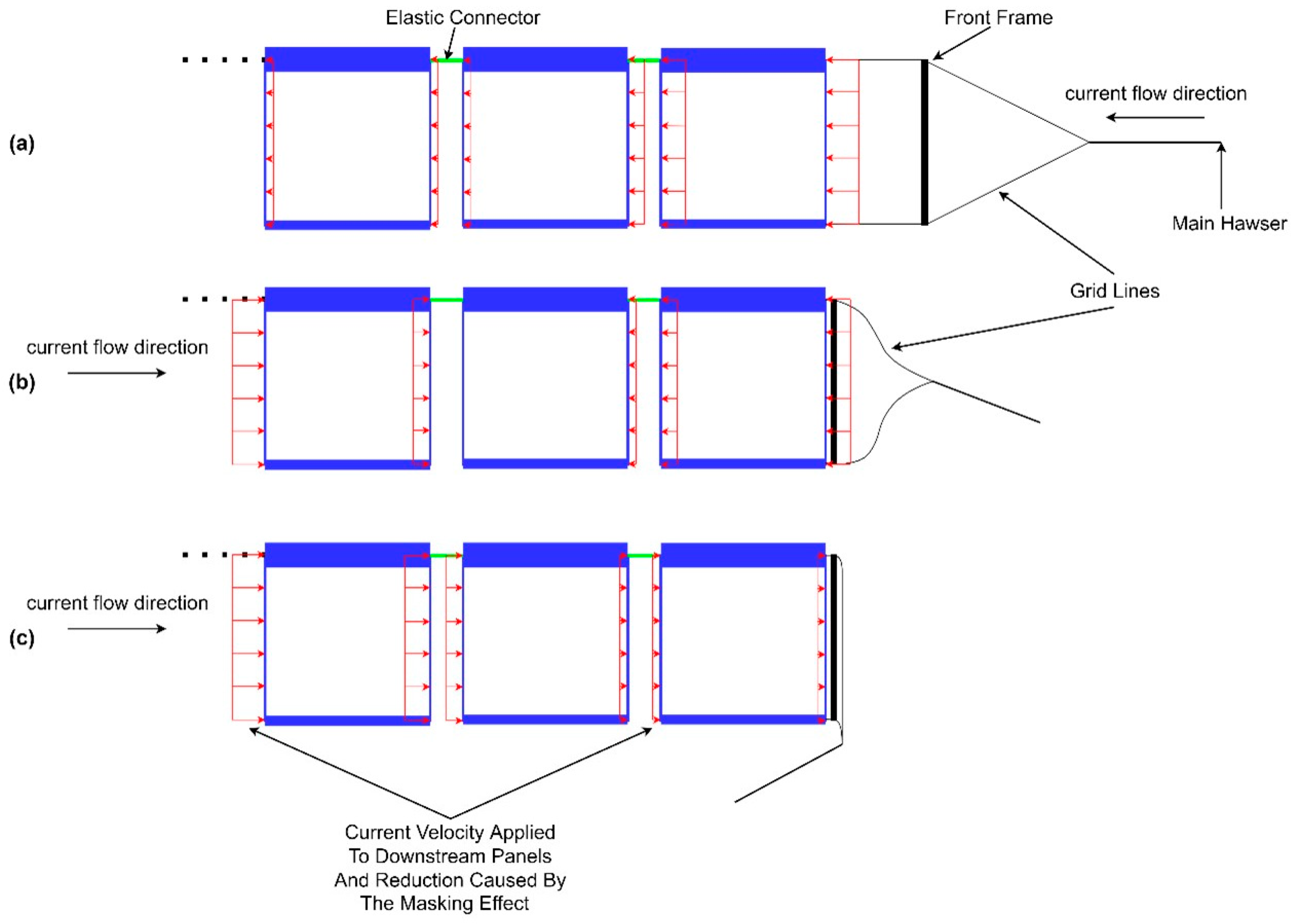
Jmse 11 00538 g002
Figure 3. A simplified vertical side schematic view of the SPM system, showing current load symbols according to current flow direction and the state of the system: (a) the initial state, where the system is tensed by the prevailing current; (b) the Drift State, where sudden opposing current starts drifting the system toward the anchor (here the load symbols shows the sum of the current loads and reacting inertia loads); (c) the holding by the anchor state, after the system drifted with no yaw rotation, until being held by the anchor line at the most unfavorable situation to buckling.
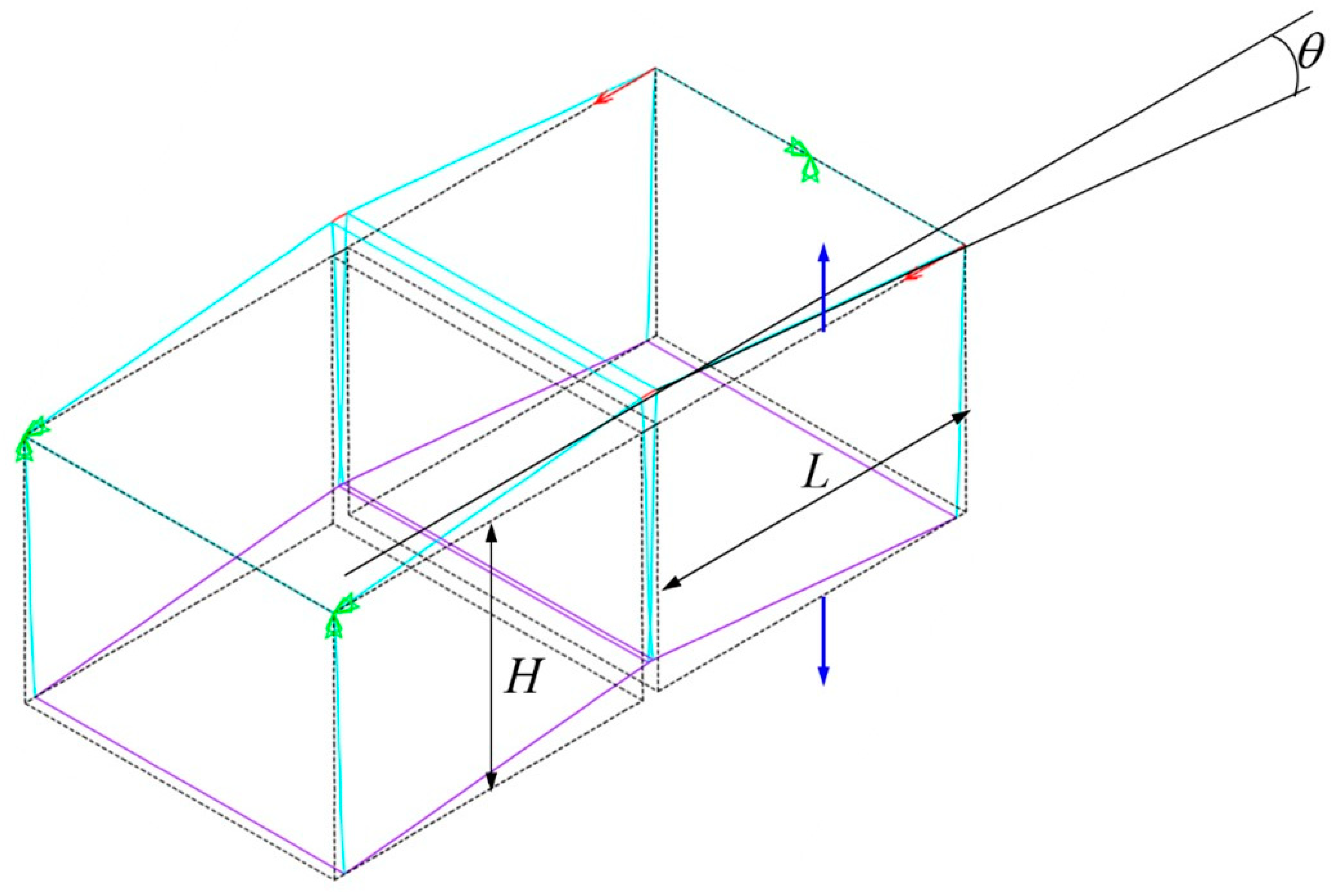
Jmse 11 00538 g003
Figure 4. Applied current and buoyancy loads FC, FB accordingly, on a cage hinged at the end, indicating the angle of pitch θ, the cage height H, and the cage length L.
Jmse 11 00538 g004
Figure 5. A schematic demonstration of the Hydrostatic Buckling and the principle of virtual work, for two connected cages. The dashed lines show the initial position of the cages while the colored solid lines present the displaced position due to Hydrostatic Buckling.
Jmse 11 00538 g005
Figure 6. Longitudinal Hydrostatic Buckling mode of a two cages system applied to a distributed current load, in the Drift State. The distributed forces are represented in red and the constraints in light blue arrows.
Jmse 11 00538 g006
Figure 7. Longitudinal buckling mode of a two cages system applied to distributed current load, in the Holding State. The distributed forces are represented in red and the constraints in light blue arrows.
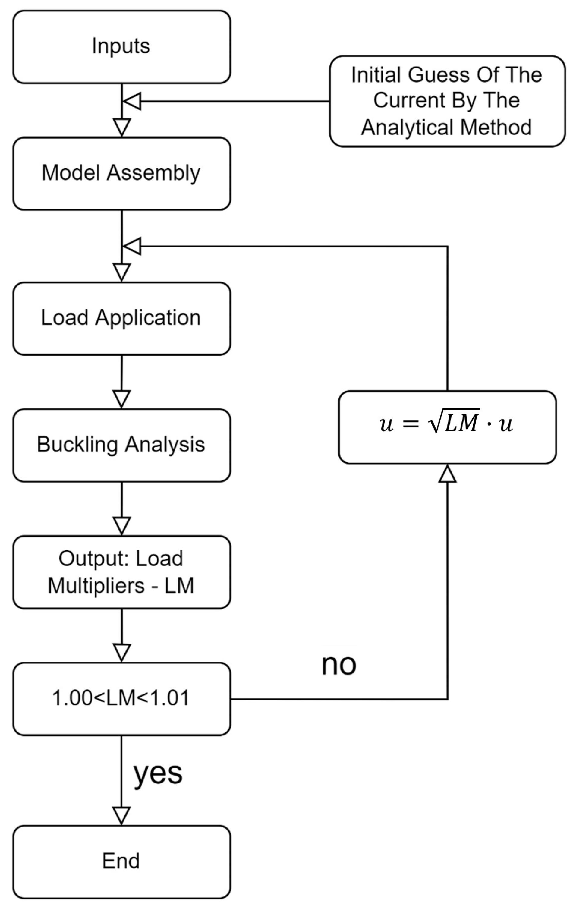
Jmse 11 00538 g007
Figure 8. Flow chart of the iterating procedure to solve the critical buckling velocity, by the APDL model.
Jmse 11 00538 g008
Figure 9. First longitudinal Hydrostatic Buckling mode for the six–cages system, in the Drift State (upper sub figure) and the Holding State (lower sub figure). The initial geometry is shown in doted black, the system’s elements, in proportional size, are in dark blue, the constraints are in a lighter blue and the drag (and reacted inertia in the Drift State) loads are shown by red arrows.
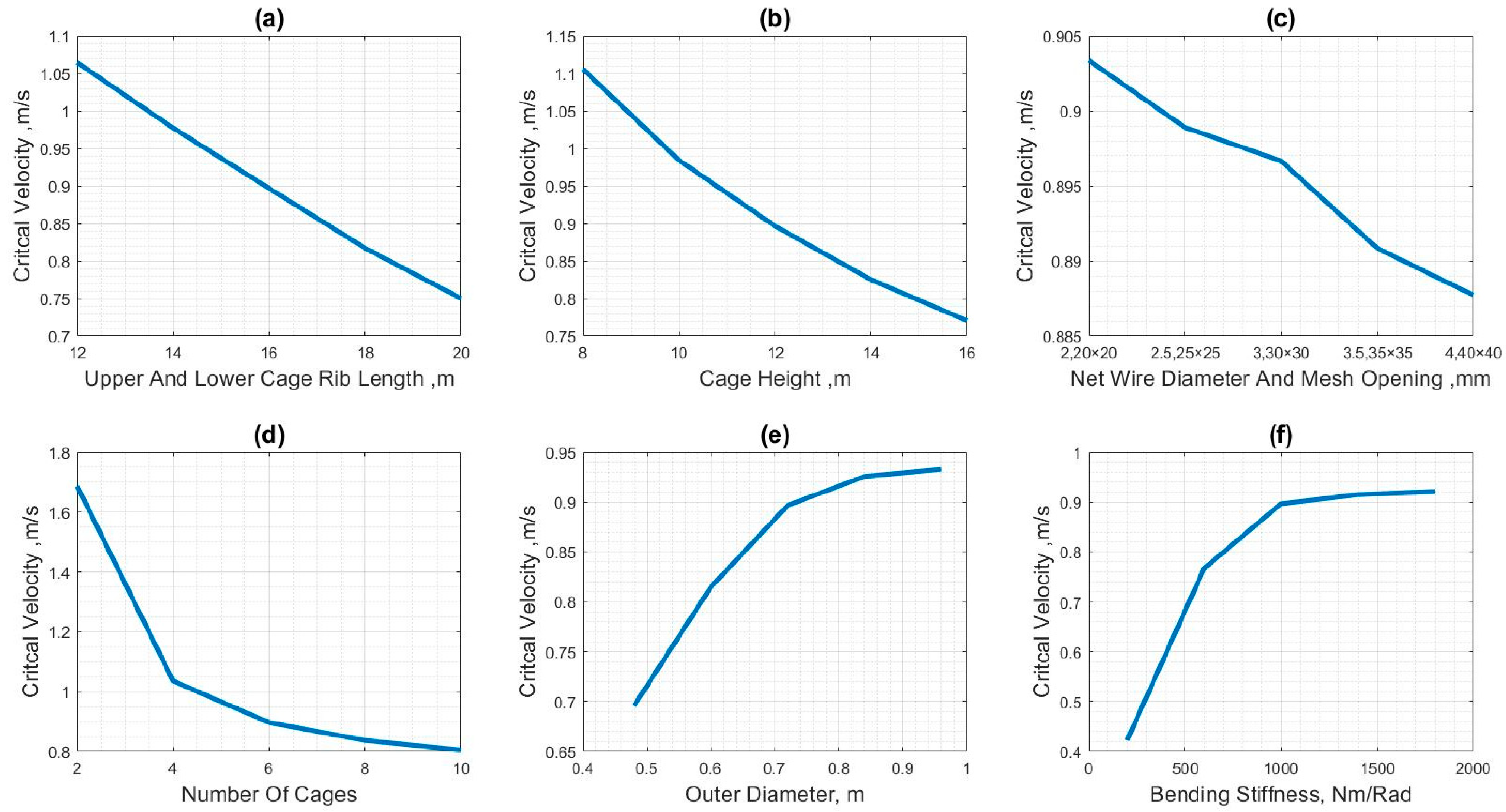
Jmse 11 00538 g009
Figure 10. The critical buckling velocity for the Drift State as a function of: (a) the cage length (and width), (b) the cage height, (c) the net mesh, (d) the number of cages, (e) the outer diameter of the upper floatation pipe and (f) the connector spring stiffness.
Jmse 11 00538 g010
Figure 11. The critical buckling velocity for the Holding State as a function of: (a) the cage length (and width), (b) the cage height, (c) the net mesh, (d) the number of cages, (e) the outer diameter of the upper floatation pipe and (f) the connector spring stiffness.
Jmse 11 00538 g011
Figure 12. The critical buckling velocity for the Drift State as a function of the cage dimension ratio H/L for combinations of N C a g e and D O 1 : (a) N C a g e = 4 ,     D O 1 = 0.6, (b) N C a g e = 6 ,   D O 1 = 0.6, (c) N C a g e = 8 ,   D O 1 = 0.6, (d) N C a g e = 4 ,   D O 1 = 0.72, (e) N C a g e = 6 ,   D O 1 = 0.72, (f) N C a g e = 8 ,   D O 1 = 0.72, (g) N C a g e = 4 ,   D O 1 = 0.84, (h) N C a g e = 6 ,   D O 1 = 0.84, (i) N C a g e = 8 ,   D O 1 = 0.84.
Jmse 11 00538 g012
Figure 13. The critical buckling velocity for the Holding State as a function of the cage dimension ratio H/L for nine combinations of N C a g e and D O 1 : (a) N C a g e = 4 ,   D O 1 = 0.6, (b) N C a g e = 6 ,   D O 1 = 0.6, (c) N C a g e = 8 ,   D O 1 = 0.6, (d) N C a g e = 4 ,   D O 1 = 0.72, (e) N C a g e = 6 ,   D O 1 = 0.72, (f) N C a g e = 8 ,   D O 1 = 0.72, (g) N C a g e = 4 ,   D O 1 = 0.84, (h) N C a g e = 6 ,   D O 1 = 0.84, (i) N C a g e = 8 ,   D O 1 = 0.84.
Jmse 11 00538 g013
Table 1. Structure parameters of the fish cage.
ComponentParameterModel
Upper Flotation Pipe
(Filled with air)
Length, L116.00 m
Diameter, DO10.720 m
Wall–Thickness, wt1 0.040 m
Vertical Connecting Pipes (filled with sea water)Height, H12.00 m
Diameter, DO30.200 m
Wall–Thickness, wt30.040 m
Lower Ballasting Pipes
(filled with sea water and ballast chain)
Length, L216.00 m
Diameter, DO20.300 m
Wall–Thickness, wt2 0.030 m
Ballast chainWeight per meter290.262 Kg/m
Copper NettingTwine Length, ltwine0.030 m
Twine Diameter, dtwine0.003 m
Elastic ConnectorLength, LC1.000 m
Diameter, DC0.100 m
Table 2. The effect of the upper and lower cage pipe length (and width) on the critical velocity, for the Drift State.
Length, mInitial Velocity by the Analytical Method, m/sCritical Velocity Assessment, m/sLoad Multiplier Factor
121.01681.0644 1.0068
14 0.93900.9772 1.0080
16 0.87600.8967 1.0031
18 0.82370.8171 1.0081
20 0.77930.7500 1.0099
Table 3. The effect of cage height on the critical velocity, for the Drift State.
Height, mInitial Velocity by the Analytical Method, m/sCritical Velocity Assessment, m/sLoad Multiplier Factor
80.89471.10551.0073
100.88540.98431.0087
120.87600.89671.0031
140.86650.82511.0091
160.85680.77051.0020
Table 4. The effect of net mesh and yarn diameter on the critical velocity, for the Drift State.
Net Mesh, mmInitial Velocity by the Analytical Method, m/sCritical Velocity Assessment, m/sLoad Multiplier Factor
2.0, 20 × 200.90160.90341.0057
2.5, 25 × 250.88890.89891.0084
3.0, 30 × 300.87600.89671.0031
3.5, 35 × 350.86290.89081.0083
4.0, 40 × 400.84970.88771.0036
Table 5. The effect of the number of cages on the critical velocity, for the Drift State.
Number of CagesInitial Velocity by the Analytical Method, m/sCritical Velocity Assessment, m/sLoad Multiplier Factor
21.72021.68601.0035
40.97051.03531.0084
60.87600.89671.0031
8 0.83810.83721.0070
100.81760.80501.0042
Table 6. The effect of the floatation pipe diameter on the critical velocity, for the Drift State.
Upper Pipe
Diameter, m
Initial Velocity by the Analytical Method, m/sCritical Velocity Assessment, m/sLoad Multiplier Factor
0.4800.47210.69591.0082
0.6000.68130.81481.0024
0.7200.87600.89671.0031
0.8401.06430.92571.0014
0.9601.24900.93291.0000
Table 7. The effect of the connector’s bending stiffness on the critical velocity, for the Drift State.
Connector Bending Stiffness, Nm/RadInitial Velocity by the Analytical Method, m/sCritical Velocity Assessment, m/sLoad Multiplier Factor
2000.87600.42261.0063
6000.87600.76701.0094
10000.87600.89671.0031
14000.87600.91501.0013
18000.87600.92131.0011
Table 8. The effect of pipe length (and width) on the critical velocity, for the Holding State.
Length, mInitial Velocity by the Analytical Method, m/sCritical Velocity Assessment, m/sLoad Multiplier Factor
12 0.76160.45391.0026
14 0.64940.41321.0078
16 0.56520.37701.0051
18 0.49980.34391.0035
20 0.44730.31571.0014
Table 9. The effect of cage height on the critical velocity, for the Holding State.
Height, mInitial Velocity by the Analytical Method, m/sCritical Velocity Assessment, m/sLoad Multiplier Factor
80.58950.46641.0014
100.57740.41461.0066
120.56520.37701.0051
140.55300.34751.0058
160.54070.32421.0007
Table 10. The effect of the net mesh and yarn diameter on the critical velocity, for the Holding State.
Net Mesh, mmInitial Velocity by the Analytical Method, m/sCritical Velocity Assessment, m/sLoad Multiplier Factor
2.0, 20 × 200.59870.38011.0071
2.5, 25 × 250.58200.37831.0083
3.0, 30 × 300.56520.37701.0051
3.5, 35 × 350.54850.37521.0045
4.0, 40 × 400.53170.37341.0031
Table 11. The effect of the number of cages on the critical velocity, for the Holding State.
Number of CagesInitial Velocity by the Analytical Method, m/sCritical Velocity Assessment, m/sLoad Multiplier Factor
21.13960.65921.0092
40.75570.45121.0048
60.56520.37701.0051
8 0.45150.33001.0019
100.37580.29561.0048
Table 12. The effect of the floatation pipe diameter on the critical velocity, Holding State.
Upper Pipe
Diameter, m
Initial Velocity by the Analytical Method, m/sCritical Velocity Assessment, m/sLoad Multiplier Factor
0.4800.16420.29161.0044
0.6000.34190.34211.0016
0.7200.56520.37701.0051
0.8400.83430.39401.0040
0.9601.14910.39891.0057
Table 13. The effect of the connector’s bending stiffness on the critical velocity, for the Holding State.
Connector Bending Stiffness, Nm/RadInitial Velocity by the Analytical Method, m/sCritical Velocity Assessment, m/sLoad Multiplier Factor
2000.56520.18251.0051
6000.56520.31221.0008
10000.56520.37701.0051
14000.56520.38331.0052
18000.56520.38461.0085
Table 14. Dimensions of the cages for studying the effect of cave dimensions ratio at constant cage volume 4096 m3.
ParameterValues Shape 1Values Shape 2Values Shape 3Values Shape 4Values Shape 5
H/L0.5000.7501.0001.2501.500
L [m]20.15917.61016.00014.85313.977
H [m]10.07913.20816.00018.56620.966
Table 15. Assessment of the critical opposing current for two systems with operational experiance.
ParameterSymbolValue Case A Value Case B
Cage Height H 12.0 [m]16.0 [m]
Cage Length L 16.0 [m]24.0 [m]
Floatation of Cage Upper Collar FB4936 [N]17,917 [N]
Critical Current Load by Equation (4)FC3702 [N]11,944 [N]
Critical current velocity u c 0.17 [m/s]0.23 [m/s]
Disclaimer/Publisher’s Note: The statements, opinions and data contained in all publications are solely those of the individual author(s) and contributor(s) and not of MDPI and/or the editor(s). MDPI and/or the editor(s) disclaim responsibility for any injury to people or property resulting from any ideas, methods, instructions or products referred to in the content.

