Abstract
Coastal defence structures play a crucial role in protecting coastal communities against extreme weather and flooding. This study investigates artificial neural network-based approaches, such as multilayer perceptron neural network (MPNN), cascade correlation neural network (CCNN), general regression neural network (GRNN), and support vector machine (SVM) with radial-bias function for estimating the wave-overtopping discharge at coastal structures featuring a straight slope ‘without a berm’. The newly developed EurOtop database was used for this study. Discriminant analysis was performed using the principal component analysis method, and Taylor diagram visualisation and other statistical analyses were performed to evaluate the models. For predicting wave-overtopping discharge, the GRNN yielded highly accurate results. As compared to the other models, the scatter index of the GRNN (0.353) was lower than that of the SVM (0.585), CCNN (0.791), and MPNN (1.068) models. In terms of the R-index, the GRNN (0.991) was superior to the SVM (0.981), CCNN (0.958), and MPNN (0.922). The GRNN results were compared with those of the previous models. An in-depth sensitivity analysis was conducted to determine the significance of each predictive variable. Furthermore, sensitivity analysis was conducted to select the optimal validation method for the GRNN model. The results revealed that both the validation methods were highly accurate, with the leave-one-out validation method outperforming the cross-validation method by only a small margin.
1. Introduction
Coastal zones have progressively developed in recent decades and have significant socioeconomic value for nations worldwide [1]. The primary objective of coastal protection infrastructure is to limit wave-induced overtopping hazards and protect people and property behind defence lines. However, the pressure on vital coastal defences is expected to increase considering the combined effects of sea level rise and increased frequency and intensity of extreme storm surges predicted for the future as a result of global climate change [2]. Although studies have been conducted on flood protection schemes for future coastal flood risk management, the risk of overtopping the crests of coastal defences must be accurately assessed while considering the uncertainties. Precise forecasting of the overland spread of wave-overtopping is crucial for the design of coastal defences [3].
Several methods have been reported for predicting the mean wave-overtopping discharge (q), which can be categorised as empirical or numerical and predicted using machine learning (ML) methods. Several ML techniques have been applied to wave-overtopping problems in recent decades. These techniques provide quick and cost-effective solutions to complex problems. The artificial neural network (ANN) model was originally created within the CLASH project (Crest Level Assessment of Coastal Structures by full-scale monitoring, neural network prediction, and hazard analysis on permissible wave-overtopping) [4] and was presented by EurOtop [5] in 2007. The ANN proposed by van Gent et al. [6] was developed as part of the CLASH project [4] and is recommended by EurOtop for predicting q values. The EurOtop (2018) [7] manual for overtopping design has provided a comprehensive review of wave-overtopping studies, and by re-analysing previously measured data, it has also investigated the relationship between the crest freeboard and mean overtopping discharge [1,8].
A special ANN tool was created by Zanuttigh et al. [9], Zanuttigh et al. [10], and Formentin et al. [11] to estimate the wave reflection coefficient Kr and wave transmission coefficients Kt and Kr, Kt, and q, respectively. In addition, Zanuttigh et al. [12] developed an enhanced ANN for various coastal structures, which was published in EurOtop (2018), with input parameters derived from an extended database [10] primarily based on the CLASH database. Molines and Medina [13] employed an ANN to derive an explicit wave- overtopping formula for breakwaters with crown walls. However, the prediction accuracy of the proposed strategy was the same as that of the CLASH-ANN. Using extended CLASH datasets, Lee [14] developed new formulae for estimating q at vertical and inclined seawalls using the group method of data handling (GMDH) algorithm. To this end, Lee and Suh [15] utilised the GMDH algorithm to develop wave-overtopping formulae for smooth and impermeable vertical seawalls. Reportedly, GMDH outperformed the empirical formulae, and its accuracy was comparable to that of the EurOtop-ANN model. Furthermore, den Bieman et al. [16] recently demonstrated that the scalable end-to-end tree-boosting system (XGBoost) method [17] could be effectively used as an alternative to ANN models. Compared with the ANN developed by van Gent et al. [6], XGBoost significantly reduced prediction errors. In addition, Hosseinzadeh et al. [18] investigated the competencies of the SVM and Gaussian process regression (GPR) methods for predicting q in simple sloped breakwaters; the models were developed using data from the EurOtop database [5]. The findings indicate that the two models, particularly the GPR model, are highly accurate. Oliver et al. [19] applied the MPNN and Kohonen neural network (KNN) to predict the overtopping rate as part of a strategy for the sustainable optimisation of coastal or harbour defence structures and their conversion into wave energy converters. Habib et al. [20] investigated the application of two advanced ML methods, a gradient-boosting-based decision tree (GBDT) and a feed-forward-based ANN framework, for predicting q in vertical breakwaters. The results revealed that the GBDT algorithm performed marginally better than the ANN algorithm. Elbisy et al. [21] evaluated the accuracy of the MPNN and random forest decision tree (RFDT) for predicting q of vertical coastal structures. They concluded that the RFDT model provided more accurate predictions than the MPNN model. Sasikumar et al. [22] used a least squares support vector machine with linear, polynomial, and radial basis function (RBF) to estimate q at a quarter-circle breakwater for varying radii and perforations. They concluded that the RBF kernel performed better than other kernels. Habib et al. [23] reviewed the use of ML to predict q and overtopping parameters. They highlighted the important limitations of the methods and identified future research needs that may serve as an impetus for the further development of these ML algorithms for wave-overtopping, particularly in applications characterised by complex geometrical configurations.
Through principal component analysis (PCA), Taylor diagram visualisation, and various evaluation indices, this study evaluated the precision of ANN algorithms, MPNN, cascade correlation neural network (CCNN), general regression neural network (GRNN), and support vector machines (SVMs) with radial bias function models to estimate q of coastal structures. Moreover, the relative significance of factors that may affect the accuracy of the models was examined in this study. The goal of this study is to provide coastal designers with a robust and accurate prediction model capable of representing wave-overtopping discharges for a wide range and types of coastal structures under various wave conditions. The MPNN was successfully utilised to predict the wave-overtopping discharge. The GRNN is simple to train and provides satisfactory prediction, modelling, mapping, and interpolation. This method is effective for continuous data analysis. An SVM is an ML model typically employed to solve regression and classification issues. In addition to effectively preventing overfitting, SVM implements structural risk minimisation.
2. Materials and Methods
2.1. ANN Methods
The multilayer perceptron is a frequently used neural network model; MPNNs generate a known output using historical data. These neural networks involve three fully interconnected layers: an input layer, at least one hidden layer, and an output layer, as shown in Figure 1. The MPNN connects all the layers using the following equation:
where w denotes the weights, b denotes the biases, f denotes the operating function, x denotes the ith input of the ANN, y denotes the jth output of the ANN, and n denotes the number of inputs [24].
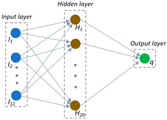
Figure 1.
Schematic diagram of an MPNN model.
In this study, a conjugate gradient algorithm was used to train the MPNN. To adjust the parameters, forward propagation (calculated loss) and back propagation (calculated derivatives) were leveraged. Transfer functions (sigmoid and linear) were used as activation functions for the hidden and output layers.
The CCNN technique was developed by Fahlman and Lebiere [25]. The CCNN has three layers and is similar to an MPNN. The primary objective of the CCNN is to expand the network structure automatically during the learning process [25]. The algorithm automatically adds and trains new neurons during the learning phase, resulting in a multi-layered structure. As the number of hidden neurons increases gradually, the training error decreases. Consequently, the training algorithm increases the complexity and generalisability of the neural network to near-optimal levels [26]. Sigmoid and linear transfer functions were used as the activation functions for the hidden and output layers, respectively.
General regression neural networks (GRNNs) are feed-forward networks that utilise a non-linear regression-based learning mechanism [27]. A typical GRNN comprises four neuron layers: input, pattern (radial basis), summation, and output (Figure 2) [28]. Notably, the number of neurons in the pattern layer is equal to that in the training data [29]. The output of the pattern layer is subsequently presented to the summation layer, which comprises numerator and denominator neurons [30]. Specifically, neurons in the summation layer are primarily responsible for summarising the output of the pattern layer. The output y-vector contains the same number of elements as the number of neurons in the numerator, which computes the weighted sum of the outputs of the neurons in the previous layer. In addition, the denominator neurons perform distinct functions. The function of this neuron is a simple summation of the outputs of the previous layer [31]. Subsequently, the sums computed by the neurons in the summation layer are divided by the neurons in the output layer. The output of the summation layer is thereafter transferred to the output layer of the predicted value (y) for an unknown input vector x expressed as [32]
where x is the input vector, xi is the ith case vector, Wi is the weight connecting the ith neuron in the pattern layer to the summation layer, and n is the number of training patterns in the input vector.
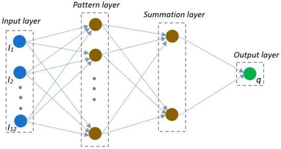
Figure 2.
Schematic diagram of a GRNN.
D denotes the Gaussian function of the following form [32]:
where xj denotes the jth input variable, xij denotes the jth data value in the ith case vector, σj denotes the smoothing factor for the ith case vector, and p denotes the number of training elements of an input vector.
2.2. SVM Method
The SVM approach was developed by Vapnik [33]. Notably, SVMs are powerful tools based on the principle of structural risk minimisation, which is a method for minimising the upper-bound risk functionally related to generalisation performance [33]. Using a non-linear mapping function, SVM maps the original input data to a higher-dimensional feature space before applying the simplest linear function to this feature space. The output estimated by SVM is expressed in the following form [33]:
where l denotes the total number of data patterns, and represent Lagrangian multipliers, corresponds to the support vector, symbolises the kernel function, and b indicates the bias term.
The kernel function employed in this study is the radial basis function (RBF),, where denotes the kernel parameter of the RBF kernel. The parameters that dominate the SVM are the coast constant (C), radius of the insensitive tube (ɛ), and the afore-mentioned kernel parameter.
Both the training subset, which was used to identify the optimal model parameters, and the validation subset were subsets of the training data. After the models were trained, they were subjected to a testing procedure to determine their efficacy in generalising the acquired knowledge to previously unexplored cases. Approximately 70% of the entire dataset was randomly selected for model training, whereas the remaining 30% was used for model testing.
Resampling techniques are generic methods for uncertainty analysis in statistics and model calibration. Resampling techniques extract several samples from a dataset and refit an assigned model on each sample to learn more about the adapted model. The most commonly used resampling methods are cross-validation and bootstrapping. According to Efron and Tibshirani [34], bootstrapping cannot detect outliers. In this study, k-fold cross-validation was used. In the k-fold cross-validation approach, a set of observations is randomly divided into k folds of approximately equal size. The first fold was treated as testing/validation of the MPNN, CCNN, and SVM, and the method was fitted on the remaining k − 1 folds. The mean squared error (MSE1) was subsequently computed from the observations in the held-out fold. This process is repeated k times (in this study, k = 10). MSE1, MSE2, …, and MSEk are the test error estimates produced by this process. The k-fold cross-validation estimate is computed by averaging these values [35]:
Each model has its own MATLAB code. Figure 3 illustrates the data pre-processing flow diagram and process modelling execution for the prediction of wave-overtopping. The statistical features listed in Table 1 were used to evaluate the different models.
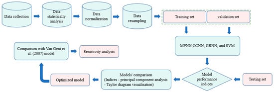
Figure 3.
Flowchart of ANN and SVM models used for wave-overtopping prediction.

Table 1.
Descriptions of the statistical features.
2.3. Data
This study utilised a newly developed EurOtop database comprising 17,942 tests, of which approximately 13,500 were solely for wave-overtopping. The original CLASH database [36] includes approximately 10,000 schematised tests on wave-overtopping discharge q, collected worldwide. The database contains 42 parameters, including 3 output parameters (q, Kr, and Kt), 11 hydraulic parameters, 23 structural parameters, and 5 general parameters. The database features a column named ‘core data’ that signifies if a test is considered part of the ‘core’ data, in which case it can be feasibly used as a training case for neural networks. This study aims to estimate the wave-overtopping discharge in coastal structures featuring a straight slope. Consequently, we only employed data from coastal structures with straight slopes, accounting for 24.53% of the EurOtop database.
In addition, the data utilised were assigned for training the ANN and SVM models. The database contains various dimensional parameters. Therefore, 12 fundamental parameters affecting the coastal structures with straight slopes were identified. Figure 4 shows a schematic of the coastal structures with a straight slope considered in this study. To summarise the characteristics of the dataset, 12 parameters and the wave-overtopping discharge were statistically measured. The statistical measures considered in this study were mathematical means, standard deviations, ranges, upper and lower 95% means, and data limits. Table 2 and Figure 5 present the statistics of the important parameters.

Figure 4.
Schematisation of the coastal structure with straight slopes [13].
Table 2.
Statistics of parameters for coastal structures with straight slopes.
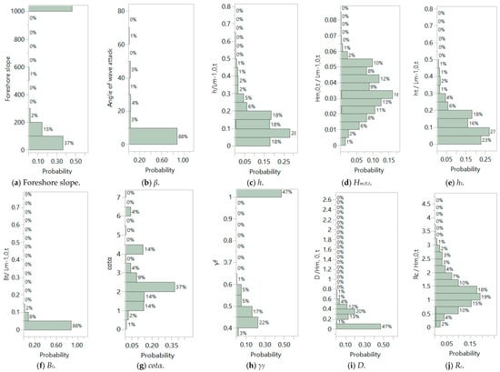
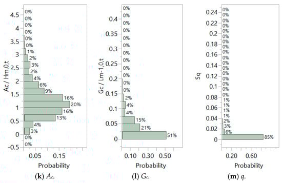
Figure 5.
Parameter spectrum of the assembled database.
To identify the gaps in the parameter values to be considered when selecting the training and testing data, these parameters were pre-analysed. Despite the wide range of available data, several limitations have been identified. The foreshore slope (m) values ranged from approximately 6 to 1000, as illustrated in Figure 5. A significant difference in the values of m was observed, which ranged from 300 to 1000. The m spectrum from 6 to 300 was covered in 54% of all the tests, whereas the spectrum from 1000 to 1100 was covered in 46% of all the tests. The angle-of-wave attack (β) and significant wave height at the structural toe (Hm, 0, t) ranged from approximately 0° to 80° and from 0.017 to 1.84 m, respectively. The β spectrum from 0° to 10° was covered in 88% of all the tests, whereas Hm,0,t was covered in 91% of all the tests for the spectrum ranging from 0.05 to 0.2 m.
As shown in Figure 5, the values of the water depth at the toe of the structure (h) and toe submergence (ht) were approximately 0.029 m and 5.01 m, respectively. The h and ht spectra from 0.029 m to 1.0 m covered 96% and 98% of all tests, respectively. When the Bt values ranged from 0 to 0.8 m, 93% of the tests values were between 0 and 0.2 m.
As shown in Figure 5, the roughness factor (γf) had a normal distribution on a scale of 0.38–1. The mean value of γf was 0.712, with 39% of tests covering the γf range between 0.4 and 0.5 and 47% of tests covering the γf range between 1.0 and 1.05. While the average size of the structure elements in the run-up/down area (D) values of all tests ranged from 0 to 0.1 m, 47% of the D values were between 0 and 0.01 m, and 50% of these values were between 0.02 and 0.08 m. Furthermore, the cotangent of the angle formed by the structure with a horizontal (cot α) value ranged from approximately 0 to 7, with 74% of all tests falling within the cot α range of 1 to 3.
The crest height with respect to the SWL (Rc) and values corresponding to the armour crest freeboard without the crown wall (Ac) ranged from approximately 0 to 2.5 m and from −0.03 to 2.5 m, respectively, as shown in Figure 5. The mean Rc value was 0.1689386 m, and 86% of the tests covered the Rc range of 0 to 0.25 m, while 12% covered the Rc range of 0.25 to 0.5. Moreover, the mean value of Ac was 0.162 m, and 87% and 12% of the tests covered an Ac ranging between 0 and 0.25 m, respectively. As shown in Figure 4, the crest width (Gc) varied between 0 and 0.1 m in 50% of all tests, while 40% of all tests covered the Gc range between 0.1 and 0.3 m.
As summarised in Figure 5 and Table 2, the wave-overtopping discharge (q) exhibited a distribution on a scale of 0.000001 m3/s per m to 0.0256 m3/s per m. The mean value and standard division of q were 0.0001 m3/s per m and 0.002 m3/s per m, respectively, and 84% of all the tests spanned the q range between 0 m3/s per m and 0.001 m3/s per m, while 6.00% of all the tests covered the q range between 0.001 m3/s per m and 0.002 m3/s per m.
3. Results and Discussion
The selection of input and output variables is one of the most crucial aspects in developing ANN and SVM models. Only 12 of the 31 parameters included in the database were selected for the creation of ANN and SVM models for overtopping prediction. The chosen parameters provide a concise overview of the overtopping discharge test. Moreover, a predetermined volume of data processing is necessary before inputting the training patterns into the network. Because certain data are obtained from small-scale models, and other data are obtained from full-scale prototypes, the new CLASH database advises against the use of basic parameters as inputs for the models. Consequently, the basic data should be dimensionless to prevent large variations in raw parameter values. Dimensionless parameters were used to improve the accuracy and reliability of the ANN and SVM models. To factor in the impacts of local breaking and wave run-up, the parameters characterising the structural heights were chosen to be dimensionless with a significant wave height. Furthermore, to account for the induced local reflection, which may or may not be in phase with the wave reflection from other portions of the structure slope, the parameters characterising the structure widths are dimensionless with respect to the wavelength [9]. Considering that the wave-overtopping rate was measured in m3/s, a scaling factor, which is the product of the length and velocity scaling factors, was required. As a result, the dimensionless wave-overtopping rate is expressed as . The dimensionless parameters are summarised in Table 3, which lists the ranges of the key parameters.
Table 3.
Input and output parameters of the ANN and SVM models.
A crucial step in the creation of any ANN and SVM technique is the choice of input and output variables; m, β, h/Lm-1,0,t, Hm,0,t/Lm-1,0,t, ht/Lm-1,0,t, Bt /Lm-1,0,t, cot α, γf, D / Hm,0,t, Rc/Hm,0,t, Ac/Hm,0,t, and Gc/Lm-1,0,t are the input variables for the ML models, and the desired output is the q. The data were scaled according to methods described by Zanuttigh et al. [10] and Formentin et al. [11].
3.1. ANN Models
The results of the MPNN and CCNN models were derived using 10-fold cross-validation based on the average results obtained for each set of test data (10-fold). In addition, a leave-one-out validation method is applied to the GRNN. The problem-specific optimal number of hidden neurons within a hidden layer is a more challenging task to manage than that of the hidden layers. If a neural network contains an excessive number of hidden neurons, it simulates random variations (noise), thereby decreasing the generalisation capacity of the neural network. Conversely, if the number of hidden neurons is insufficient, the converse situation occurs. The neural network fails to approximate the desired outcome, thereby preventing generalisation. Neural networks that cannot be generalised lose their utility because they perform optimally only with their training data. A genetic algorithm (GA) was employed to adjust the optimal size of the MPNN. Interestingly, the MPNN analysis revealed that a hidden-layer network featuring 20 neurons could form an optimal and stable network. The training parameters of the MPNN model are listed in Table 4.
Table 4.
Model parameters of the ANN and SVM models.
For the predicted wave-overtopping of the MPNN model, MSE = 0.000001, MAE = 0.001, RMSE = 0.001, SI = 1.068, Ef = 0.843, and R = 0.922, with a maximum error of 0.007. Figure 6 and Figure 7 show the relationships between the actual and predicted values of wave- overtopping based on the ANN and SVM models.
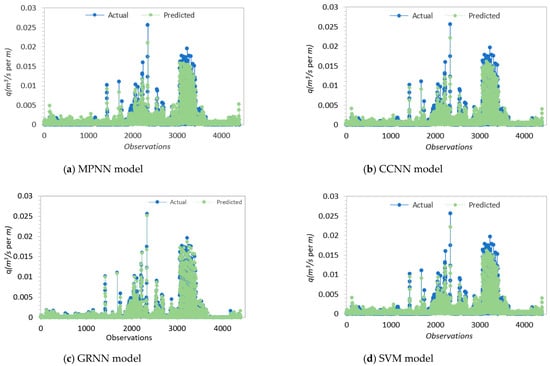
Figure 6.
Plot of the measured and predicted values of wave-overtopping.
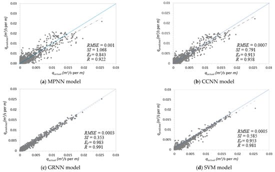
Figure 7.
Scatter plots of the measured and predicted wave-overtopping values for various models.
Using a CCNN training scheme, the wave-overtopping prediction was performed for another iteration. This iteration was performed to determine whether using a different algorithm could improve the training results. Table 4 lists the training parameters for the CCNN model. For the predicted wave-overtopping, MSE = 0.000001, MAE = 0.0004, RMSE = 0.0007, SI = 0.791, Ef = 0.913, and R = 0.958, and a maximum error of 0.005 was obtained from the training data. The findings indicate that CCNN offers several advantages over MPNN, including quick learning, network self-determination of size and topology, retention of built-in structures even when the training set is altered, and lack of backpropagation of error signals through the connections of the network.
The training parameters of the GRNN model are listed in Table 4. In addition, Table 5 lists the ideal sigma (σ) for each input parameter corresponding to the GRNN model. The results show that the predicted wave-overtopping discharge has an MSE of 0.0000001, MAE of 0.0001, RMSE of 0.0003, SI of 0.353, Ef = 0.983, R of 0.991, and a maximum error of 0.0026. Based on the experimental findings, the predicted values are relatively close to the corresponding measured values.
Table 5.
Optimal sigma values for each input parameter of the GRNN model.
3.2. SVM Model
When using an SVM, the foremost consideration is the selection of the kernel function. Because of the strong nonlinear dynamics of the wave-overtopping phenomena, a nonlinear kernel function can outperform a linear kernel function. In this study, the RBF was employed as the kernel function of the SVM because it performs optimally under general assumptions of smoothness. This performance was demonstrated by comparing the RBF results with those of the polynomial and sigmoid kernel functions. The performance of the SVMs constructed using the sigmoid or polynomial basis kernel functions was not superior to that constructed using the radial basis kernel function. The polynomial kernel performed worse and required more time for the SVM training. Secondly, the values of the free parameters of the radial basis kernel function must be determined. The performance of the SVM was significantly influenced by parameter selection. Notably, the impact of selecting these parameters on the resulting generalisation errors is worth investigating.
These parameters must be carefully selected to ensure an efficient model. In this study, the optimal values of the SVM parameters (, C, , and P) were determined using an SVM grid-and-pattern search, with the adjusted parameters with the lowest validation errors being chosen as the optimal parameters. Subsequently, the SVM model was trained using optimal parameters. The adjusted parameters with the lowest validation errors were selected as the optimal parameters. Subsequently, the SVM model was trained using optimal parameters. Table 4 lists the parameter values for the various SVM models. The relationship between the predicted and actual wave-overtopping discharge values obtained using the SVM model is plotted in Figure 6 and Figure 7. The results were as follows: maximum error = 0.005, MSE = 0.0000002, MAE = 0.0003, RMSE = 0.0005, and SI = 0.585. The R and Ef values were 0.981 and 0.953, respectively.
3.3. Comparison between the ANN and SVM Models
The predictions made using the ANN and SVM models were compared, and the results are presented in this section. Figure 8 shows the relationship between the observed and predicted wave-overtopping values using various models. A continuous diagonal line served as a reference. The actual wave-overtopping at any point along this reference line was identical to that predicted by the different models for a certain observation. If the predicted wave-overtopping values fell below this reference line, the model was considered conservative. However, if these values lied above the reference line, the model was considered to have overestimated wave-overtopping. To enhance the clarity of the figure, a trend line was drawn for the results of the ANN and SVM models and compared with the diagonal reference line.
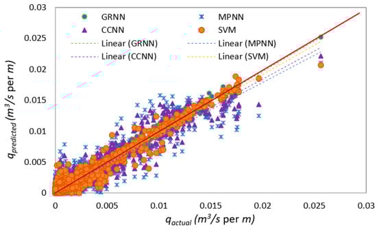
Figure 8.
Scatter plot of measured and predicted wave-overtopping values for the ANN and SVM models.
Generally, a model is more accurate or effective in predicting wave-overtopping if the discrete points lie closer to the trend line. The trend line for the GRNN model was close to the reference line. The trend lines for the SVM and CCNN were the second and third closest to the reference line, respectively, following the trend line for the GRNN model, as revealed by a visual comparison of the trend lines of the various models with the reference line illustrated in Figure 8. Numerous CNN, SVM, and GRNN points were situated above the reference line, indicating that these models grossly overestimated the wave-overtopping at these points. Because the trend line corresponding to the MPNN model is the furthest from the reference line, and all its points are located far from the reference line, the MPNN model underestimated the parameters the most for predicting the wave-overtopping of the different samples.
In addition, discriminant analysis was conducted using the PCA method to investigate the relationship between the outcomes of the ANN and SVM models and the actual wave-overtopping discharge (q (actual)). Table 6 illustrates the contribution of each variable to the first five principal components, their corresponding eigenvalues, and the cumulative variance. Table 7 lists the extracted eigenvectors for the ANN and SVM models and q (actual). Using analysis of the correlation circle, which corresponds to a projection of the initial variables of the first two PCA factors onto a two-dimensional plane, correlations between q (actual) and ANN, and SVM models were revealed, and the axes or main factors could be interpreted. As shown in Figure 9, a strong correlation exists between q (actual) and the predictions yielded by the GRNN, SVM, and CCNN models. The results of the GRNN model exhibit a higher correlation with q (actual) than those of the other models, indicating that it reduces the overall errors in the predictions of the wave-overtopping discharge. Therefore, the GRNN model can predict wave-overtopping discharge with greater accuracy and reliability. Discriminant analysis using the PCA method revealed that the MPNN exhibited the worst performance in terms of predicting wave-overtopping discharge.
Table 6.
Eigenvalues of the correlation matrix.
Table 7.
Extracted eigenvectors for actual wave-overtopping discharge and ANN and SVM models.
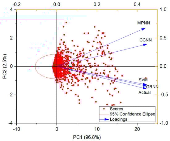
Figure 9.
PCA for the actual wave-overtopping discharge and ANN and SVM models.
The Taylor diagram provides a graphical representation of the suitability of various ANN and SVM models based on R, RMSE, and standard deviation (Figure 10). A Taylor diagram is a two-dimensional space in which predicted, and actual values are positioned according to their degree of coordination. The standard deviation, RMSE, and R2 score are each represented by the horizontal and vertical axes, circular lines, and radial lines, respectively. The accuracy of a model is measured by the proximity of each model to the actual value. The closer a prediction model is to the actual data, the more reliable it is. The GRNN model, which has a higher R2 score and standard deviation and a lower RMSE than the SVM model, is closer to the actual values and, as shown schematically in Figure 10, is marginally more reliable.
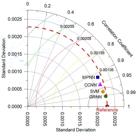
Figure 10.
Taylor diagram visualization of ANN and SVM model performance.
The GRNN model exhibited superior prediction performance in terms of MSE, MAE, RMSE, SI, Ef, and R values, while SVM was the second-best model (Table 8). In terms of predicting the wave-overtopping discharge, the results demonstrate that the performance of the GRNN model was superior to that of the other models. In addition, the results indicated that the GRNN model substantially reduced the overall error and accurately predicted wave-overtopping discharge. The MPNN model exhibited the worst predictive performance, indicating that it could not accurately represent wave-overtopping discharge. Overall, the results demonstrate that the GRNN model outperformed the other ANN models. Furthermore, the high accuracy of the GRNN and SVM models was validated by the results.
Table 8.
Error statistics for different ANN and SVM models.
Compared to the other models, the GRNN produced SI values that were 202.66%, 124.08%, and 65.72% lower than those of the MPNN, CCNN, and SVM, respectively (Figure 11). Furthermore, the RMSE of the GRNN was 210.35%, 131.03%, and 68.96% lower than those of the MPNN, CCNN, and SVM, respectively. In terms of Ef, the GRNN outperformed the MPNN, CCNN, and SVM by 16.61%, 7.67%, and 3.15%, respectively (Figure 11). Generally, the outcomes of the GRNN model were more accurate than those of the other models. Essentially, the GRNN model accurately predicts the wave-overtopping discharge. In terms of predictive accuracy, speed, convenience, and interpretability, the results demonstrate that the GRNN is the most reliable model for predicting wave-overtopping discharge.
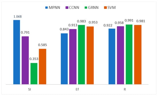
Figure 11.
Comparison of the different ANN and SVM models.
3.4. Comparison of the GRNN Model with the van Gent et al. (2007) Model
To validate the GRNN model, its performance was compared with the ANN model proposed by van Gent et al. [6]. According to the results, the MSE, MAE, RMSE, SI, Ef, and R of the two models demonstrate the superior performance of the GRNN model. In addition, the results indicate that the GRNN model significantly reduced the overall error and accurately estimated the wave-overtopping discharge. The RMSE of the GRNN model was lower than that of the van Gent et al. model, which was 0.0003 and 0.0005, respectively. Furthermore, the SI calculated using the GRNN model (0.353) was lower than that calculated by van Gent et al. (0.989). The trend line for the GRNN model was closer to that of the ANN model by van Gent et al. (2007), as revealed by a visual comparison of the trend lines of the two models with the reference line illustrated in Figure 7 and Figure 12.
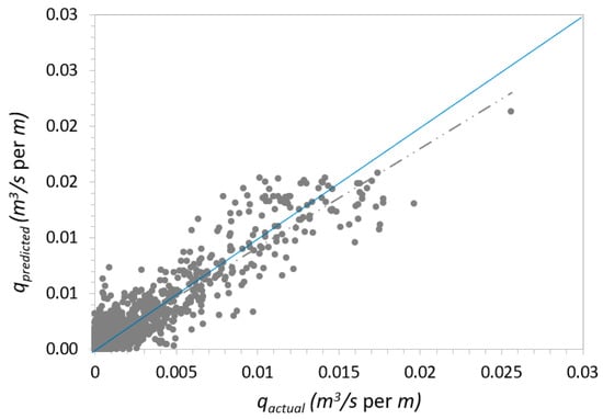
Figure 12.
Scatter plot of the measured and predicted wave-overtopping values of the ANN model by van Gent et al. (2007).
In this study, the significance of the predictor variables in the GRNN model was determined through cross-validation. Sensitivity analysis was employed in the calculation, where the values of each variable were randomised, and the impact on the quality of the model was assessed. The analysis revealed that Rc/Hm,0,t (28.24%) was the most significant predictor, followed by Hm,0,t/Lm-1,0,t (14.17%), h / Lm-1,0,t (13.52%), ht/Lm-1,0,t (12.83%), Ac/Hm,0,t (9.45%), Bt / Lm-1,0,t (6.41%), β (6.39%), cot αd (5.29%), Gc/Lm-1,0,t (2.22%), D/ Hm,0,t, m (0.7%), and γf (0.08%).
In addition to determining the optimal configuration of the input vectors, the model optimisation procedure included a calibration phase to precisely define the optimal validation method for the GRNN model. The performance of the GRNN was compared using cross-validation and leave-one-out validation techniques, and the results are presented in this section. The compositions of the two validation methods are shown in Figure 13. The results confirmed the high accuracy of the two validation methods; however, the accuracy of the leave-one-out validation method was slightly higher than that of the cross-validation method.
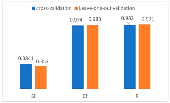
Figure 13.
Comparison of the cross-validation and leave-one-out validation methods for the GRNN model.
4. Conclusions
In this study, the application of ANN and SVM models (MPNN, CCNN, GRNN, and SVM) to the prediction of wave-overtopping discharge was refined and compared with the ANN developed by van Gent et al. [5]. The ML-based models were trained using the EurOtop database (4401 data points). The ANN and SVM models were characterised by 12 predictors of the 31 parameters included in the database. An in-depth sensitivity analysis was performed for each parameter to determine the best input pattern. Rc/Hm,0,t (28.24%) was found to be the most significant predictor, followed by Hm,0,t/Lm-1,0,t (14.17%), h / Lm-1,0,t (13.52%), ht/Lm-1,0,t (12.83%), Ac/Hm,0,t (9.45%), Bt /Lm-1,0,t (6.41%), β (6.39%), cot αd (5.29%), Gc/Lm-1,0,t (2.22%), D/ Hm,0,t, m (0.7%), and γf (0.08%).
PCA, Taylor diagram visualisation, and six statistical features were used to assess the predictive performances of the various ANN and SVM models. The GRNN yielded highly accurate results in terms of estimating wave-overtopping discharge. The SI of the GRNN (0.353) was lower than those of the SVM (0.585), CCNN (0.791), van Gent et al. (0.989), and MPNN (1.068) models. In addition, the Ef of the GRNN (0.983) was higher than that of the SVM (0.953), CCNN (0.913), van Gent et al. (0.865), and MPNN (0.843) models. The results revealed that the GRNN model substantially reduced the overall error and accurately estimated the wave-overtopping discharge. Compared to the ANN developed by van Gent et al. [6], the GRNN model significantly reduced prediction errors. This result demonstrates its superior accuracy and precision compared with the other models. Further research should be conducted to accurately represent more complex geometries (coastal structures with a berm) in the GRNN model. Furthermore, comparisons should be made with other available prediction methods for the wave-overtopping discharge.
Author Contributions
Conceptualization, M.S.E.; methodology, M.S.E.; software, M.S.E. and A.H.A.; validation, M.S.E. and A.H.A.; formal analysis, M.S.E.; investigation, M.S.E.; resources, Alshahri; data curation M.S.E.; writing—original draft preparation, M.S.E. and A.H.A.; writing—review and editing, M.S.E.; visualization A.H.A.; supervision, M.S.E.; project administration, A.H.A.; funding acquisition, A.H.A. All authors have read and agreed to the published version of the manuscript.
Funding
This research was funded by Taif University Deanship of Scientific Research Project, grant number (1-443-5).
Data Availability Statement
Not applicable.
Acknowledgments
The authors would like to express their appreciation to the referees of the paper for their critical review, as well as their valuable comments that improved the paper to its present form.
Conflicts of Interest
The authors declare no conflict of interest. The funders had no role in the design of the study; in the collection, analyses, or interpretation of data; in the writing of the manuscript, or in the decision to publish the results.
References
- Dong, S.; Abolfathi, S.; Salauddin, M.; Tan, Z.H.; Pearson, J.M. Enhancing climate resilience of vertical seawall with retrofitting-A physical modelling study. Appl. Ocean. Res. 2020, 103, 102331. [Google Scholar] [CrossRef]
- Salauddin, M.; O’Sullivan, J.J.; Abolfathi, S.; Peng, Z.; Dong, S.; Pearson, J.M. New insights in the probability distributions of wave-by-wave overtopping volumes at vertical breakwaters. Sci. Rep. 2022, 12, 16228. [Google Scholar] [CrossRef] [PubMed]
- Mehrabani, M.B.; Chen, H.-P.; Stevenson, M.W. Overtopping failure analysis of coastal flood defences affected by climate change. J. Phys. Conf. Ser. 2015, 628, 12049. [Google Scholar] [CrossRef]
- De Rouck, J.; Van de Walle, B.; Geeraerts, J. Crest level assessment of coastal structures by full scale monitoring, neural network prediction adn hazard analysis on permissible wave overtopping-(CLASH). Proc. Eurocean 2004, 2004, 1–4. [Google Scholar]
- Pullen, T.; Allsop, N.W.H.; Bruce, T.; Kortenhaus, A.; Schüttrumpf, H.; Van der Meer, J.W. EurOtop Wave Overtopping of sea Defences and Related Structures: Assessment Manual. 2007. Available online: http://www.overtopping-manual.com/assets/downloads/EAK-K073_EurOtop_2007.pdf (accessed on 14 December 2022).
- van Gent, M.R.A.; van den Boogaard, H.F.P.; Pozueta, B.; Medina, J.R. Neural network modelling of wave overtopping at coastal structures. Coast Eng. 2007, 54, 586–593. [Google Scholar] [CrossRef]
- EurOtop, Manual on Wave Overtopping of Sea Defences and Related Structures, 2nd ed. 2018. Available online: http://www.overtopping-manual.com/assets/downloads/EurOtop_II_2018_Final_version.pdf (accessed on 14 December 2022).
- Dong, S.; Salauddin, M.; Abolfathi, S.; Pearson, J. Wave impact loads on vertical seawalls: Effects of the geometrical properties of recurve retrofitting. Water 2021, 13, 2849. [Google Scholar] [CrossRef]
- Zanuttigh, B.; Formentin, S.M.; Briganti, R. A neural network for the prediction of wave reflection from coastal and harbor structures. Coast Eng. 2013, 80, 49–67. [Google Scholar] [CrossRef]
- Zanuttigh, B.; Formentin, S.M.; Van der Meer, J.W. Advances in Modelling Wave-Structure Interaction Through Artificial Neural Networks. Coast Eng. Proc. 2014, 1, 69. [Google Scholar] [CrossRef]
- Formentin, S.M.; Zanuttigh, B.; Van Der Meer, J.W. A neural network tool for predicting wave reflection, overtopping and transmission. Coast Eng. J. 2017, 59, 1750006-1–1750006-31. [Google Scholar] [CrossRef]
- Zanuttigh, B.; Formentin, S.M.; van der Meer, J.W. Prediction of extreme and tolerable wave overtopping discharges through an advanced neural network. Ocean. Eng. 2016, 127, 7–22. [Google Scholar] [CrossRef]
- Molines, J.; Medina, J.R. Explicit wave overtopping formula for mound breakwaters with crown walls using CLASH neural network-derived data. J. Waterw. Port. Coast. Ocean Eng. 2016, 142, 4015024. [Google Scholar] [CrossRef]
- Lee, S.B. Derivation of Wave Overtopping Formulas for Vertical and Inclined Seawalls Using GMDH Algorithm. Master’s Thesis, Seoul National University, Seoul, Republic of Korea, 2018. [Google Scholar]
- Lee, S.B.; Suh, K.-D. Development of wave overtopping formulas for inclined seawalls using GMDH algorithm. KSCE J. Civ. Eng. 2019, 23, 1899–1910. [Google Scholar] [CrossRef]
- den Bieman, J.P.; van Gent, M.R.A.; van den Boogaard, H.F.P. Wave overtopping predictions using an advanced machine learning technique. Coast Eng. 2021, 166, 103830. [Google Scholar] [CrossRef]
- Chen, T.; Guestrin, C. Xgboost: A scalable tree boosting system. In Proceedings of the 22nd Acm Sigkdd International Conference on Knowledge Discovery and Data Mining, San Francisco, CA, USA, 13–17 August 2016; pp. 785–794. [Google Scholar]
- Hosseinzadeh, S.; Etemad-Shahidi, A.; Koosheh, A. Prediction of mean wave overtopping at simple sloped breakwaters using kernel-based methods. J. Hydroinform. 2021, 23, 1030–1049. [Google Scholar] [CrossRef]
- Oliver, J.M.; Esteban, M.D.; López-Gutiérrez, J.-S.; Negro, V.; Neves, M.G. Optimizing wave overtopping energy converters by ANN modelling: Evaluating the overtopping rate forecasting as the first step. Sustainability 2021, 13, 1483. [Google Scholar] [CrossRef]
- Habib, M.A.; O’Sullivan, J.; Salauddin, M. Comparison of machine learning algorithms in predicting wave overtopping discharges at vertical breakwaters. In Proceedings of the EGU General Assembly 2022, Vienna, Austria, 23–27 May 2022. [Google Scholar]
- Elbisy, M.S.; Osra, F.A.; Alyafei, Y.S. Soft computing techniques for predicting wave overtopping discharges at vertical coastal structures. GEOMATE J. 2022, 23, 205–211. [Google Scholar] [CrossRef]
- Sasikumar, H.; Mane, V.; Rao, S. Estimation of Wave Overtopping Discharge at Quarter Circle Breakwater Using LSSVM. In Proceedings of 2nd International Conference on Artificial Intelligence: Advances and Applications: ICAIAA 2021; Springer: Berlin/Heidelberg, Germany, 2022; pp. 399–405. [Google Scholar]
- Habib, M.A.; O’Sullivan, J.J.; Salauddin, M. Prediction of Wave Overtopping Characteristics at Coastal Flood Defences Using Machine Learning Algorithms: A Systematic Rreview. In IOP Conference Series: Earth and Environmental Science; IOP Publishing: Philadelphia, PA, USA, 2022; p. 12003. [Google Scholar]
- Swingler, K. Applying Neural Networks: A Practical Guide. In Morgan Kaufmann; Morgan Kaufman Publishers: San Francisco, CA, USA, 1996. [Google Scholar]
- Fahlman, S.; Lebiere, C. The cascade-correlation learning architecture. Adv. Neural. Inf. Process Syst. 1989, 2, 524–532. [Google Scholar]
- Song, J.; Romero, C.E.; Yao, Z.; He, B. A globally enhanced general regression neural network for on-line multiple emissions prediction of utility boiler. Knowl. Based Syst. 2017, 118, 4–14. [Google Scholar] [CrossRef]
- Specht, D.F. A general regression neural network. IEEE Trans. Neural. Netw. 1991, 2, 568–576. [Google Scholar] [CrossRef]
- Ye, H.; Ren, Q.; Hu, X.; Lin, T.; Shi, L.; Zhang, G.; Li, X. Modeling energy-related CO2 emissions from office buildings using general regression neural network. Resour. Conserv. Recycl. 2018, 129, 168–174. [Google Scholar] [CrossRef]
- Antanasijević, D.Z.; Ristić, M.Đ.; Perić-Grujić, A.A.; Pocajt, V.V. Forecasting human exposure to PM10 at the national level using an artificial neural network approach. J. Chemom. 2013, 27, 170–177. [Google Scholar] [CrossRef]
- Ni, Y.Q.; Li, M. Wind pressure data reconstruction using neural network techniques: A comparison between BPNN and GRNN. Measurement 2016, 88, 468–476. [Google Scholar] [CrossRef]
- Kisi, O.; Tombul, M.; Kermani, M.Z. Modeling soil temperatures at different depths by using three different neural computing techniques. Theor. Appl. Climatol. 2015, 121, 377–387. [Google Scholar] [CrossRef]
- Barzegar, R.; Asghari Moghaddam, A. Combining the advantages of neural networks using the concept of committee machine in the groundwater salinity prediction. Model. Earth Syst. Environ. 2016, 2, 26. [Google Scholar] [CrossRef]
- Vapnik, V.; Golowich, S.; Smola, A. Support vector method for function approximation, regression estimation and signal processing. Adv. Neural. Inf. Process Syst. 1996, 9, 1–7. [Google Scholar]
- Efron, B.; Tibshirani, R.J. An Introduction to the Bootstrap; CRC Press: Boca Raton, FL, USA, 1994. [Google Scholar]
- James, G.; Witten, D.; Hastie, T.; Tibshirani, R. An Introduction to Statistical Learning; Springer: Berlin/Heidelberg, Germany, 2013; Volume 112. [Google Scholar]
- van der Meer, J.W.; Verhaeghe, H.; Steendam, G.J. The new wave overtopping database for coastal structures. Coast Eng. 2009, 56, 108–120. [Google Scholar] [CrossRef]


Disclaimer/Publisher’s Note: The statements, opinions and data contained in all publications are solely those of the individual author(s) and contributor(s) and not of MDPI and/or the editor(s). MDPI and/or the editor(s) disclaim responsibility for any injury to people or property resulting from any ideas, methods, instructions or products referred to in the content. |
© 2023 by the authors. Licensee MDPI, Basel, Switzerland. This article is an open access article distributed under the terms and conditions of the Creative Commons Attribution (CC BY) license (https://creativecommons.org/licenses/by/4.0/).