Abstract
Trajectory tracking control of unmanned surface vessels (USVs) has become a popular topic. Regarding the problem of ship collision avoidance encountered in trajectory tracking, more attention needs to be paid to the algorithm application, namely the characteristics of flexibility and accessibility. Thus, a fusion framework of field theoretical planning and a model predictive control (MPC) algorithm is proposed in this paper to obtain a realizable collision-free tracking trajectory, where the trajectory smoothness and collision avoidance constraints under a complex environment need to be considered. Through the designed fast matching (FM) method based on the electric field model, the algorithm gains the direction trend of collision avoidance planning and then combines it with a flexible distance to reconstruct the architecture of the MPC and constraint system, generating the optimal trajectory tracking controller. The new algorithm was tested and validated for several situations, and it can potentially be developed to advance collision-free trajectory tracking navigation in multivessel situations.
1. Introduction
The tracking control of an unmanned surface vessel (USV) is the key factor in determining the effect of autonomous navigation, mainly measured by the trajectory smoothness, angle realizability, attitude fluctuation, tracking time, etc., affecting the complexity and accessibility of the controller. In addition, in an actual sea area, it is necessary to consider collision avoidance regarding surrounding ships and to dynamically adjust the trajectory to adapt to a complex environment of multiple vessels. Therefore, the control of a USV needs to achieve trajectory tracking and collision avoidance [1,2].
In the existing literature, it is customary to divide collision avoidance trajectory planning and tracking control into two parts that take global or local path planning as tracking parameters combined with an appropriate control algorithm to design a control rate to realize trajectory tracking and navigation. Therefore, classical trajectory planning algorithms based on geometric models [3], potential field models [4], velocity obstacle models [5], environmental dynamic interaction models [6], and classical algorithms for control, such as adaptive control [7], model predictive control (MPC) [8], sliding mode control [9], anti-disturbance control [10], and intelligent heuristic control [11], can be used in conjunction with each other according to different requirements. For example, Shen et al. [12] formulated the path planning problem into a receding horizon optimization framework with spline path templates to obtain the local optimal path and then used a nonlinear MPC to achieve the tracking goal. Tor et al. [13] planned route compliance with the Convention on the International Regulations for Preventing Collisions at Sea (COLREGs) and hazard evaluation criterion on a finite horizon to select the optimal behavior for an MPC. Namgung [14] further analyzed various encounter scenarios in COLREGs to put forward a local route planning method using a fuzzy inference system based on near collision, ship domain, and velocity obstacle models. Zheng et al. [15] used the Kalman filter and collision risk index to predict a ship’s trajectory and then sought the steering angle via an improved cultural particle swarm optimization algorithm. Huang et al. [16] constructed a framework of a human–machine interaction-oriented collision avoidance system to gain the decision-making trajectory, cooperating with a PD controller to complete automatic navigation. Husain et al. [17] discussed cooperative path-planning and tracking controller for autonomous vehicles using a distributed MPC approach. Xu et al. [18] considered the direction of resultant velocity under a Frenet frame to solve the problem about static or slow time-varying obstacles and used an MPC to track the planned motion.
The above distribution scheme of planning and control is easier to use and has a large scale for algorithm transplantation and improvement. Nevertheless, the weak coupling and correlation between control parameters and planning states, especially for real-time collision avoidance scenarios, increase the target complexity and reduce the control accessibility. Therefore, some research literature on the fusion scheme of planning and control has been published accordingly. Miele et al. [19] discussed the strategy for the ship collision avoidance of optimal control that maximizes the timewise minimum distance based on the multiple-subarc sequential gradient-restoration algorithm with respect to the controls. Tomas et al. [20] proposed a decentralized collision avoidance system that directly mixes the control problem for multi-UAV scenarios. Zhou et al. [21] listed four steps of the collision avoidance process and determined the optimal maneuvers of each step to obtain a suitable control state. All of the above are basically planning designs integrated in the control algorithm, which are also referred to in this paper, but they ignore the practicality of the control algorithm.
To realize the application of the algorithm, it needs to be based on a control algorithm suitable for the integration control of the fusion framework. It is well known that MPC specializes in solving engineering control problems and has excellent iterative, optimization, and prediction performance, also known as receding horizon control [22,23]. Therefore, the MPC architecture is considered for the tracking control of USVs. Currently, there is a single type of research on MPC collision avoidance, mostly designed to improve the cost function [24] or to add fixed distance constraints [25] to obstacle avoidance. To optimize the collision avoidance constraints, Mohamed [26] employed the COLREGs to give the constraint restrictions in different modes of USVs for circular ship domains and elliptical ship domains, which are more coherent with actual ship handling specifications. Inger [27] argued for the hazard evaluation criterion of collision avoidance on the basis of the COLREG constraints. In addition, Eriksen et al. [28] introduced the pseudo-Huber cost function into the MPC method, and Julien et al. [29] designed a trade-off cost function incorporating obstacle avoidance, reference trajectory tracking, and control energy. All of them set a fixed range of collision avoidance areas, lacked a detailed collision avoidance planning strategy, and used only a single distance dimension. Moreover, Icaro et al. [30] introduced a dynamical collision cost function into the cost function of MPC, but it used a hierarchical scheme with the planning layer and tracking controller layer. Salim et al. [31] proposed soft and hard constraints for the MPC problem to address collision and obstacle avoidance about the formation control of a multiple quadcopter. Both of them provide a trend of development. Therefore, the flexible cost function and multi-dimensional collision avoidance constraints need to be considered and integrated into MPC tracking control. Here, the field method [32,33], which is mathematically elegant and incorporates simple path planning, is integrated into MPC control to compensate for the information of the direction dimension for collision avoidance constraints, and a soft margin is set for the distance cost function in this paper, which achieves the goal of balancing the path redundancies and energy costs.
In summary, to address the difficulty of handling the mutual incoordination of collision avoidance planning and control execution, a fusion framework of field theoretical planning and an MPC algorithm was built that can carry out trajectory tracking and real-time collision avoidance under engineering constraints to realize autonomous navigation in a multivessel environment. This approach has the following advantages over the existing solutions: (1) The fusion framework enhances the coupling relationship between trajectory planning and control action, reduces the redundant influence of ship maneuvering parameters, and executes uniform tracking control regarding the relevant state parameters of ship motion, not just the location state. (2) The collocation of MPC and the field model helps form a tracking path with a reachable angle and smooth trajectory, taking into account the trend of collision avoidance, without the exact collision avoidance path. (3) The flexibility and accessibility of control algorithms encountered in trajectory tracking is improved, which combines the manipulation constraints and trend of avoidance control, strengthening the potential relationship between collision avoidance planning and control. (4) The integrated control of multiobjective dimensions is proposed that is beneficial to coordinate and regulate in line with the trend of collision avoidance. The main novelties are that the direction trend judgment of collision avoidance planning is obtained through the design of a new fast matching (FM) method based on an electric field model and that the direction trend and elastic distance are introduced into the collision avoidance constraint of MPC for the first time rather than a fixed distance range, which broadens the state dimension, obtaining better performance. The position change is dynamically described by the backpropagation of the ship motion when considering the collision avoidance constraint; moreover, the more simplified trajectory tracking control algorithm combined with collision avoidance action is designed to balance the complexity and accuracy to obtain a reliable route. In short, it provides a new idea for the coordinated implementation of trajectory control and collision avoidance strategy.
The rest of this paper is organized as follows. In Section 2, the problem formulation is given. Section 3 presents the detailed methodologies of controller design. The simulation experiments under different complex scenes are presented in Section 4. Finally, the conclusion of this paper is in Section 5.
2. Problem Formulation
Ship tracking navigation is the key phase in ship autonomous navigation systems, which includes navigation, guidance, and control [34]. It is necessary not only to ensure the consistency of the tracking preset trajectory but also to consider maneuverability and to choose the optimal tracking route with low redundancy and energy loss. Therefore, from the point of view of ship kinematics and dynamics models [35], the state is controlled to sail to the expected trajectory, and an underactuated surface ship with three degrees of freedom is considered here, whose functions are determined by
where , in which u, v, and r are the surge, sway, and yaw velocity, respectively, in the body-fixed frame; x and y are the positions in the earth-fixed frame; is the yaw angle; is the force in the surge; and is the moment of the yaw. The inertia components are m11, m22, and m33, and d11, d22, and d33 are the damping components. (as shown in Figure 1).
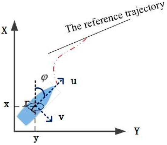
Figure 1.
Ship motion structure.
Under the given expected trajectory , trajectory tracking is realized by finding a control law to make
However, for the actual dynamic environment, to prevent collision, the tracking trajectory is adjusted, and the following two requirements should be focused on: (1) the path loss of the adjusted trajectory should be reduced, and the expected tracking status should be restored as soon as possible; (2) the smoothness of the adjusted track should have control accessibility, and the adjustment should be realized normally under the physical constraints of the USV.
Therefore, defining state and control , Formula (1) is transformed into:
The aim is to design a real-time trajectory tracking controller based on MPC and field theory for the above system and to avoid obstacle ships.
3. Controller Design
3.1. Model Predictive Control Scheme
MPC has been maturely applied in engineering control to find the optimal target based on a finite-horizon cost, where a receding horizon strategy is used to continuously iterate and update, and the handling of state and control variables are constrained to make the algorithm model more relevant to the actual scenario. This necessitates a model describing the dynamic behavior of a plant whose function is to predict the future dynamics of the system, emphasizing the predictive effect of the model, rather than the form, so that it is suitable for objective online optimization and extreme value programming [36].
The continuous-time model (3) needs to be discretized and described as . For the optimization problem of tracking control under a given expected condition, the cost function can be obtained by
Here, represents the forward i-step prediction of the state at time instant k, and represents the forward i-step of the expected tracking state at time instant k. Analogously, is the forward i-step prediction of the control input at time instant k, and is the forward i-step of the expected control input at time instant k. Step N is the terminal horizon.
Ignoring the avoidance problem, at time instant k, the optimization problem can be formulated as
are the state and control input constraints, whose scopes are set according to the specific conditions of ship navigation. Solving the optimal control input of the MPC scheme, the ship tracks and optimizes according to the set trajectory and finally maintains the state of Formula (2).
3.2. Collision Avoidance
- (1)
- Fast matching method based on the electric field model
Facing the situation of uncertainty and complexity in collision avoidance, field theory is used for avoidance planning. Currently, usually the artificial virtual field method is used to construct the target surrounding field state, but this method cannot describe the intership effect and cannot fully represent the sailing change of the ship, so the use of the electric field model for ship state simulation, where the superposition effect can be expressed well, was proposed [37]. Through the spatial electric field mode, the field energy state of the ship itself and the influence of the ship-to-ship effect are established. To describe each ship as a point charge, the collision level around the ship is represented using the equipotential surface formed by the field energy generated by the electric field model. With increasing distance, the collision avoidance level decreases and so does the collision risk; the equivalent model can be expressed as:
where is the field energy, QS is the quality of the ship, is a constant parameter, and r is the distance between the surrounding point and the center of the ship.
With the advantage of the superimposed effect of field energy, this is a good representation of the vector field distributed in the space waters of multiple vessels, which is also the base vector field of the FM method carrying out collision avoidance planning.
FM is an energy-efficient path planning method that sets a target point and combines the gradient descent algorithm. This method has the features of a global minimum and no local minima problem, decreasing the computational burden. Its aim is to generate an arrival time map that satisfies the Eikonal equation, which describes a wave front propagation scenario in the base vector field E. The Eikonal equation can be written as:
where is the arrival time of wave propagation at position , and is the speed of wave propagation at position . Taking the energy cost into account, the minimum arrival time is chosen as the best path trend [38]. The planned path of the algorithm is shown below.
In Figure 2, the path is planned with the current position of the ship as the starting point (red point) in the presence of two obstacle ships. The color bar shows the level of the energy field. It is obvious that the trajectory is affected by the energy field generated by the two obstacle ships, and the trajectory is updated with the movement of the ships’ positions.
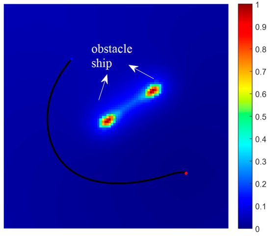
Figure 2.
The planned path.
However, the collision avoidance path obtained by the above method is not the final path that the USV needs to follow, and it is necessary to readjust the original tracking trajectory combined with the MPC controller in Section 3.1.
- (2)
- Integration of collision avoidance planning into MPC
According to the MPC architecture, the collision avoidance strategy is integrated from the two aspects of the cost function and constraint conditions. The constraint conditions are considered first. The direction dimension is considered in the constraint rather than just using a fixed range for the distance constraint. The novel collision avoidance constraint includes two points: the direction trend from the FM method based on the electric field model indirectly gives the possible adjustment direction of the predicted trajectory and the distance limit between the ship and obstacle ship at the same time, as depicted in Figure 3.
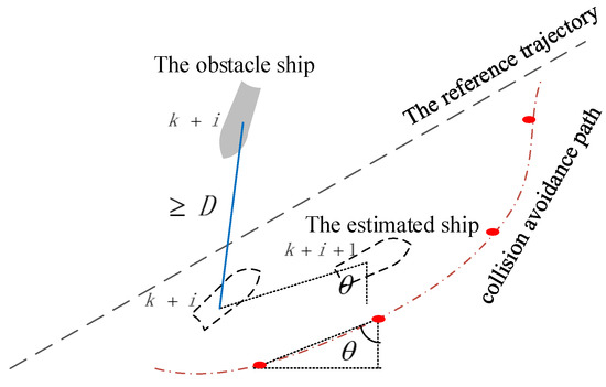
Figure 3.
The distance correlation model between the ship and obstacle ship.
Figure 3 reveals the distance limitation between the obstacle ship and the estimated position of the ship, which is affected by the trend selection of collision avoidance planning through a correlation of . The collision avoidance trajectory obtained from Section 3.1 is divided according to the prediction horizon N, and the value of the trajectory point corresponding to each sampling interval is found, and , namely, is the orthogonal ratio of the adjacent trajectory points. The estimated position of the ship at the current time is indicated by backpropagating the estimated position at the next moment.
Therefore, the collision avoidance inequality constraint is as follows for each obstacle ship j ():
where is the sample time; , , , and correspond to x, y, u, and v of the estimated ship state, respectively; xta and yta are the positions of obstacle ships; M is the total number of obstacle ships; and D is the safe distance of collision avoidance. This constraint focuses on applying the trend of collision avoidance planning to state optimization, which guides the direction of the estimated trajectory and limits the position by setting a safe distance.
Harsh constraints result in an increase in computational complexity, and there exist some path loss and redundancy when the predicted states of N steps are all required to meet the limitation of D; therefore, an additional slack variable is added into the cost function, which also expands the solution-seeking space. The new cost function is listed as:
Here, , is a segmented constant, which varies with the positive or negative value of the distance difference in dis(k + i). If the distance difference is negative, it is negative; otherwise, it is positive. The new component indicates a soft margin regarding distance setting, which advantageously introduces the elastic factor to balance the hard conditions brought by the constraints.
Furthermore, the variable factor is considered in the safe distance D, as opposed to a fixed value based on experience, where the empirical formula for the minimum safe encounter distance is introduced as an elastic variable, drawing on the report of Li [39].
where D0 is the distance constant, and is the relative azimuth, which stands for the angle between the ship velocity and the distance from the ship to the obstacle ship.
Thus, Formulas (8) and (9) integrate collision avoidance planning into the MPC method to solve the problem of obstacle ship avoidance during autonomous trajectory tracking. After collision avoidance is complete, the ship trajectory returns to the previously expected tracking route.
3.3. Optimization Problem and Algorithm
The important factors for the optimal control problem are parameter selection and computational efficiency. An increasing number of constraints and objectives increase the computational burden of the traditional algorithm. Therefore, we transform the optimal control problem into a nonlinear programming problem, whose core idea is to use the system model as the state constraint of each optimization step. To achieve better computing efficiency and a faster running time, the CasADi tool proposed for nonlinear optimization and algorithmic differentiation is chosen to solve this optimization problem, which has features of rapid and efficient nonlinear MPC.
The whole structure of USV trajectory tracking is as follows in Figure 4:
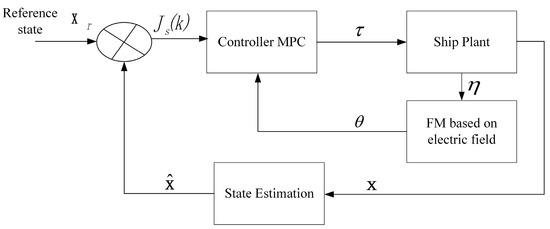
Figure 4.
The tracking structure.
The algorithm flow of tracking control is given in Algorithm 1.
| Algorithm 1: | The algorithm process |
| Inputs: | The reference state x of tracked trajectory |
| Outputs: | The estimated state x of ship trajectory tracking |
| Procedure: | if no obstacle ships with constraints as Formula (5) in current time k. else calculate the direction trend about FM based on electric field model. bring into the formula (8) and combine the Formula (9) to reconstruct the cost function with the collision avoidance constraint in current time k. end if find the optimal solution of input control u using CasADi. compare the next state x with the reference state xr. At next time, instant repeat procedure |
3.4. Stability Analysis
Here, the stability of the proposed MPC structure is verified by Lyapunov functions, which satisfies the following theorem.
Theorem 1.
If there exists a continuously differentiable scalar function V(x) such that:
- (1)
- is positive definite
- (2)
We consider the minimization of the predicted infinite horizon cost [40]:
where .
Assumption 1 is observable in the sense that
for some finite , is any matrix
with
According to Assumption 1, it is known that for getting , meaning that is positive definite.
Considering an infinite horizon, the is followed:
Then, is suboptimal at time k + 1; meanwhile, the obstacle ship is detected in a certain distance range Dd, so it has
Therefore, the stability of the algorithm is guaranteed.
4. Simulation
4.1. Simulation Parameters
The damping components of the ship system are , and other hydrodynamic parameters are selected depending on Cui et al. [41]. The parameters involved in the MPC method are selected as follows: the sample step in simulation unit is T = 0.1(), prediction horizon N = 8, , , and . The thrust is within the interval of [−400, 400], and the moment is within the interval of [−100, 100]. The initial state of the ship is , and the expected tracking trajectory is set to . Then, USV tracking control for different multivessel scenarios conforming to Algorithm 1 is simulated. Here, we use two algorithms for comparison with the proposed algorithms. The influence on the trajectory when using the fixed distance as the obstacle avoidance constraint shown in Formula (15), called the original algorithm, is observed, and the multiobjective programming model of the distance at closest point of approach (DCPA) and time at closest point of approach (TCPA), with reference to Li et al. [37], are used to replace the collision avoidance trend angle , called the compared algorithm, and are compared.
where = 1.5.
4.2. Results
- (1)
- Single obstacle ship
The trajectory of the obstacle ship is set to , and the results of the three algorithms are obtained.
The superiority of the new algorithm is expressed in Figure 5a, where the course and trajectory adjustment occur at the time range of t30–t50, but for the new algorithm, the change is obviously better than those of the original algorithm and the compared algorithm, indicating that the direction trend and elastic strategy have a certain effect. The comparison of the input control, that is, the thrust, is given in Figure 5b, which shows that the fluctuations caused by tracking the expected trajectory are relatively frequent in the initial stage, where the effects of the three algorithms are exactly the same, and fluctuations produce differences when collision avoidance is required. The new algorithm reaches the expected trajectory state immediately after a small adjustment, and the changes of other states with the new algorithm are shown in Figure 5c, all of which achieve the expected state very well.
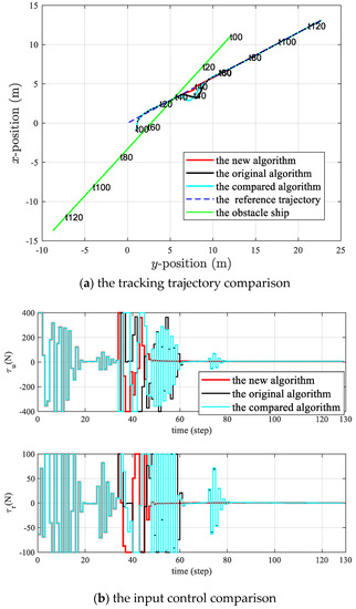
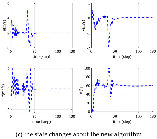
Figure 5.
Comparison of algorithms under single obstacle ship.
- (2)
- Multivessel environment
The following focuses on collision avoidance when multiple vessels meet at the same time. The tracking situations of the two algorithms are given in Figure 6a–c, where two obstacle ships with states and are encountered simultaneously. The collision avoidance adjustment is mainly concentrated in the range between t10 and t80; in this stage, the new algorithm needs to avoid two obstacle ships at the same time and triggers larger fluctuations in the trajectory, corresponding to the changes in u, v, r, and states reflected in (c). The fluctuations are smaller in the late t80 period, which is mainly affected by one obstacle ship. The compared and original algorithms have more oscillations than the new algorithm throughout the whole period and are still adjusting when the new algorithm has tracked the expected trajectory, as shown in (b), and have worse smoothness than the new algorithm.
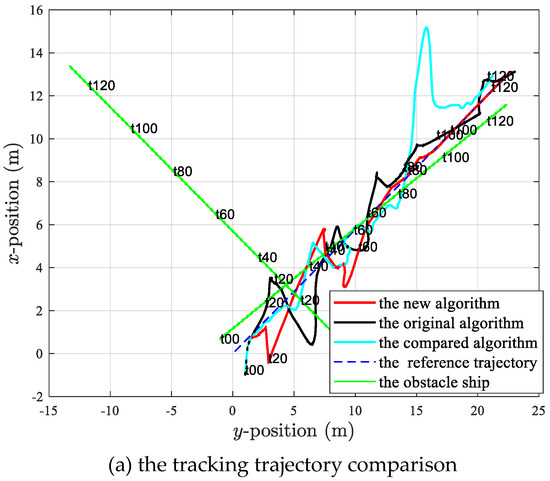
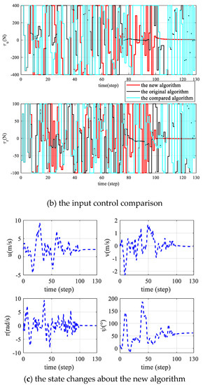
Figure 6.
Comparison of algorithms under two obstacle ships.
The displayed trajectory and state changes with an obstacle ship with state , in addition to the above two obstacle ships, are depicted in Figure 7a,c. The adjustment of the new algorithm is concentrated between t10 and t60, where the amplitude and smoothness of fluctuations are better than those of the original algorithm, and the adjustment range of the thrust is smaller than that of the original algorithm (see (b)). However, the difference between the comparison algorithm and the new algorithm is not obvious; the new algorithm is adjusted ahead of the comparison algorithm, and the thrust is weaker in the later stage.
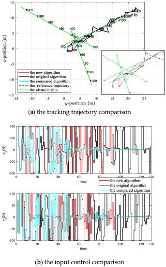
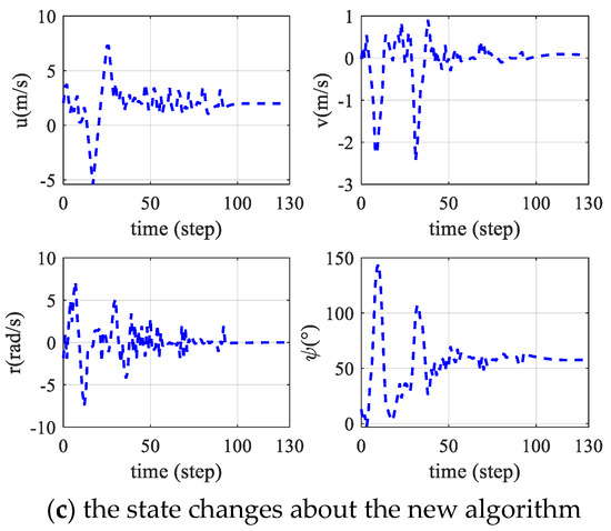
Figure 7.
Comparison of algorithms under three obstacle ships.
Furthermore, the performance when a fourth obstacle ship with state rendezvous with the others at the same time is described in Figure 8. With the increase in the number of obstacle ships, there is a greater impact on the collision avoidance complexity, and the adjustment range is obviously larger than that in Figure 7, but the overall status is prior to the original algorithm, although the adjustment time increases. The fluctuations of the compared algorithm are greater than those of the new ones. Although the collision avoidance planning in the compared algorithm is more accurate than that of the new ones, it is not conducive to the overall tracking of the integrated controller, and the new algorithm has certain advantages in trajectory trend and state tracking, which has a better trajectory performance for slow fluctuations in the overall situation.
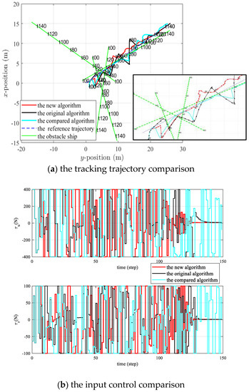
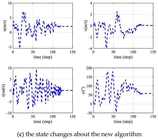
Figure 8.
Comparison of algorithms under four obstacle ships.
In brief, considering the direction dimension of the collision avoidance constraint and the elastic distance of the cost function, the new algorithm is an improvement of the MPC method and has lower complexity, easier angle realizability, less attitude fluctuations, and shorter tracking time, especially in the case of multiple vessels meeting simultaneously, obtaining a better balance between the complexity and accessibility of the controller.
5. Conclusions
A novel fusion algorithm for trajectory tracking was proposed that creates a controller based on MPC-integrated collision avoidance planning whose structure uses the direction trend generated by the FM method of the electric field model and flexible distance to design the collision avoidance constraints and the cost function of the MPC controller. Then, the CasADi method was used for fast optimization to realize the trajectory tracking target during real-time collision avoidance adjustment. A collision-free trajectory that balances efficiency and accuracy was obtained through the fusion framework proposed in this study, which focused on coordinating control execution and collision avoidance planning while considering manipulation constraints. The framework met the parameter requirements for algorithm flexibility and accessibility and exhibits excellent performance under harsh environments where multiple vessels meet simultaneously.
The proposed algorithm provides a solution to the fusion control process for considering the multidimensional trend of collision avoidance, and cross-fuses the collision avoidance decision-making and trajectory control modules in intelligent navigation rather than just providing control input parameters. At the same time, the field model was used to avoid the complex structure of collision avoidance decision-making, but it also brings deficiencies in decision accuracy and trajectory redundancy. Other elements of collision avoidance decision need to be added to optimize this structure, such as energy cost not being satisfactory; and some practical factors still need to be given in the future, such as the COLREGs and collision avoidance actions of obstacle ships, which can be solved by introducing game theory and other methods. In addition, some environmental interferences can be added to the field model to form a more comprehensive control impact. Therefore, further enhancement is necessary to improve this fusion algorithm.
Author Contributions
Conceptualization, Y.P.; methodology, Y.L.; writing—review and editing, Y.P. All authors have read and agreed to the published version of the manuscript.
Funding
This research is supported by the National Natural Science Foundation of China under Grant 51909155 and Shanghai High-level Local University Innovation Team (Maritime safety and technical support).
Institutional Review Board Statement
Not applicable.
Informed Consent Statement
Not applicable.
Data Availability Statement
Not applicable.
Conflicts of Interest
The authors declare no conflict of interest.
References
- Huang, Y.M.; Chen, L.Y.; Chen, P.F.; Rudy, R.N.; Gelder, P.H.A.J.M. Ship collision avoidance methods: State-of-the-art. Saf. Sci. 2020, 121, 451–473. [Google Scholar] [CrossRef]
- Akdağ, M.; Solnør, P.; Johansen, T.A. Collaborative collision avoidance for maritime autonomous surface ships: A review. Ocean Eng. 2022, 250, 110920. [Google Scholar] [CrossRef]
- Tsou, C.M.; Kao, S.L.; Su, C.M. Decision Support from Genetic Algorithms for Ship Collision Avoidance Route Planning and Alerts. J. Navig. 2020, 63, 167–182. [Google Scholar] [CrossRef]
- Wang, T.F.; Yan, X.P.; Wang, Y.; Wu, Q. Ship Domain Model for Multi-ship Collision Avoidance Decision-making with COLREGs Based on Artificial Potential Field. Int. J. Mar. Navig. Saf. Sea Transp. 2017, 11, 85–92. [Google Scholar] [CrossRef]
- Zhao, Y.; Li, W.; Shi, P. A real-time collision avoidance learning system for unmanned surface vessels. Neurocomputing 2016, 182, 255–266. [Google Scholar] [CrossRef]
- Xie, S.; Chu, X.M.; Zheng, M.; Liu, C.G. A composite learning method for multi-ship collision avoidance based on reinforcement learning and inverse control. Neurocomputing 2020, 411, 375–392. [Google Scholar] [CrossRef]
- Guo, M.C.; Xu, D.B.; Liu, L. Adaptive nonlinear ship tracking control with unknown control direction. Int. J. Robust Nonlinear Control. 2018, 28, 2828–2840. [Google Scholar] [CrossRef]
- Li, H.P.; Yan, W.S.; Shi, Y. Continuous-time model predictive control of under-actuated spacecraft with bounded control torques. Automatica 2017, 75, 144–153. [Google Scholar] [CrossRef]
- Liu, Y.; Bu, R.X.; Gao, X.R. Ship Trajectory Tracking Control System Design Based on Sliding Mode Control Algorithm. Pol. Marit. Res. 2018, 25, 26–34. [Google Scholar] [CrossRef]
- Li, Y.; Bai, X.E.; Xiao, Y.J. ship course sliding mode control system based on a novel extended state disturbance observer. J. Shanghai Jiao Tong Univ. 2014, 48, 1708–1713. [Google Scholar] [CrossRef]
- Alejandro, R.M.; Efrén, M.M.; Miguel, G.V.C.; Mario, A.P. Multi-objective meta-heuristic optimization in intelligent control: A survey on the controller tuning problem. Appl. Soft Comput. 2020, 93, 106342. [Google Scholar] [CrossRef]
- Shen, C.; Shi, Y.; Brad, B. Integrated Path Planning and Tracking Control of an AUV: A Unified Receding Horizon Optimization Approach. IEEE/ASME Trans. Mechatron. 2017, 22, 1163–1173. [Google Scholar] [CrossRef]
- Tor, A.J.; Tristan, P.; Andrea, C. Ship Collision Avoidance and COLREGS Compliance Using Simulation-Based Control Behavior Selection With Predictive Hazard Assessment. IEEE Trans. Intell. Transp. Syst. 2016, 17, 3407–3422. [Google Scholar] [CrossRef]
- Namgung, H. Local Route Planning for Collision Avoidance of Maritime Autonomous Surface Ships in Compliance with COLREGs Rules. Sustainability 2022, 14, 198. [Google Scholar] [CrossRef]
- Zheng, Y.S.; Zhang, X.G.; Shang, Z.J.; Guo, S.Y.; Du, Y.Q. A Decision-Making Method for Ship Collision Avoidance Based on Improved Cultural Particle Swarm. J. Adv. Transp. 2021, 2021, 8898507. [Google Scholar] [CrossRef]
- Huang, Y.M.; Chen, L.Y.; Rudy, R.N.; Gelder, P.H.A.J.M. A ship collision avoidance system for human-machine cooperation during collision avoidance. Ocean Eng. 2020, 217, 107913. [Google Scholar] [CrossRef]
- Kanchwala, H.; Viana, I.B.; Aouf, N. Cooperative path-planning and tracking controller evaluation using vehicle models of varying complexities. Proc. Inst. Mech. Eng. Part C J. Mech. Eng. Sci. 2021, 235, 2877–2896. [Google Scholar] [CrossRef]
- Xu, H.; Zhang, X.K. Tracking control of ship at sea based on MPC with virtual ship bunch under Frenet frame. Ocean Eng. 2022, 247, 110737. [Google Scholar] [CrossRef]
- Miele, A.; Wang, T. Maximin Approach to the Ship Collision Avoidance Problem via Multiple-Subarc Sequential Gradient-Restoration Algorithm. J. Optim. Theory Appl. 2005, 124, 29–53. [Google Scholar] [CrossRef]
- Tomas, B.; Daniel, H.; Giuseppe, L.; Martin, S.; Vijay, K. Model Predictive Trajectory Tracking and Collision Avoidance forReliable Outdoor Deployment of Unmanned Aerial Vehicles. In Proceedings of the IEEE/RSJ International Conference on Intelligent Robots and Systems (IROS) Madrid, Spain, 1–5 October 2018; pp. 6753–6760. [Google Scholar]
- Zhou, K.; Chen, J.H.; Liu, X. Optimal Collision-Avoidance Manoeuvres to Minimise Bunker Consumption under the Two-Ship Crossing Situation. J. Navig. 2018, 71, 151–168. [Google Scholar] [CrossRef]
- Shen, C.; Shi, Y.; Brad, B. Path-Following Control of an AUV: A Multiobjective Model Predictive Control Approach. IEEE Trans. Control. Syst. Technol. 2019, 27, 1334–1342. [Google Scholar] [CrossRef]
- Yan, X.P.; Wang, S.W.; Ma, F.; Liu, Y.C.; Wang, J. A novel path planning approach for smart cargo ships based on anisotropic fast matching. Expert Syst. Appl. 2020, 159, 113558. [Google Scholar] [CrossRef]
- Zhou, C.; Lei, M.; Zhou, S.L.; Zhang, W.G. Collision-free UAV Formation Flight Control based on Nonlinear MPC. In Proceedings of the IEEE International Conference on Electronics, Ningbo, China, 3 November 2011; pp. 1951–1956. [Google Scholar]
- Da, L.; Cao, Q.; Xian, Y.Q.; Gao, Y.L. Distributed MPC for formation of multi-agent systems with collision avoidance and obstacle avoidance. J. Frankl. Inst. 2017, 354, 2068–2085. [Google Scholar] [CrossRef]
- Mohamed, E.H.A. Nonlinear Model Predictive Control for Trajectory Tracking and Collision Avoidance of Surface Vessels. Doctoral Dissertation, Carl von Ossietzky university, Oldenburg, Germany, 2018. [Google Scholar]
- Inger, B.H. Collision Avoidance for ASVs Using Model Predictive Control. Master’s Thesis, Norwegian University of Science and Technology, Trondheim, Norway, 2017. [Google Scholar]
- Eriksen, B.O.H.; Breivik, M. MPC-based Mid-level Collision Avoidance for ASVs using Nonlinear Programming. In Proceedings of the IEEE Conference on Control Technology and Applications (CCTA), Kohala Coast, HI, USA, 27–30 August 2017; pp. 766–772. [Google Scholar]
- Julien, M.; Sylvain, B.; Alexandre, E.; Martial, S.; Julien, M. Reactive MPC for Autonomous MAV Navigation in Indoor Cluttered Environments: Flight Experiments. IFAC-PapersOnLine 2017, 50, 15996–16002. [Google Scholar] [CrossRef]
- Viana, I.B.; Kanchwala, H.; Ahiska, K.; Aouf, N. A comparison of trajectory planning and control frameworks for cooperative autonomous driving. J. Dyn. Syst. Meas. Control. 2021, 143, 071002. [Google Scholar] [CrossRef]
- Vargas, S.; Becerra, H.M.; Hayet, J.-B. MPC-based distributed formation control of multiple quadcopters with obstacle avoidance and connectivity maintenance. Control. Eng. Pract. 2022, 121, 105054. [Google Scholar] [CrossRef]
- Mauro, M.; Nicoletta, B.; Elisa, C.; Elisabetta, P. Sliding Mode Control Techniques and Artificial Potential Field for Dynamic Collision Avoidance in Rendezvous Maneuvers. IEEE Control Syst. Lett. 2020, 4, 313–318. [Google Scholar]
- Sun, X.J.; Wang, G.F.; Fan, Y.S.; Mu, D.D.; Qiu, B.B. An Automatic Navigation System for Unmanned Surface Vehicles in Realistic Sea Environments. Appl. Sci. 2018, 8, 193–220. [Google Scholar] [CrossRef]
- Lazarowska, A.; Żak, A. A Concept of Autonomous Multi-Agent Navigation System for Unmanned Surface Vessels. Electronics 2022, 11, 2853. [Google Scholar] [CrossRef]
- Fossen, T. Guidance and Control of Ocean Vehicles; Wiley Interscience: New York, NY, USA, 1994; ISBN 978-0-471-94113-2. [Google Scholar]
- Lars, G.; Jürgen, P. Nonlinear Model Predictive Control-Theory and Algorithms; Springer: London, UK; Dordrecht, The Netherlands; Heidelberg, Germany; New York, NY, USA, 2011; ISBN 978-0-85729-500-2. [Google Scholar]
- Li, Y.; Zheng, J. Real-time Collision Avoidance Planning for Unmanned Surface Vessels Based on Field Theory. ISA Trans. 2020, 106, 233–242. [Google Scholar] [CrossRef]
- Song, R.; Liu, Y.C.; Richard, B. A multi-layered fast matching method for unmanned surface vehicle path planning in a time-variant maritime environment. Ocean Eng. 2017, 129, 301–317. [Google Scholar] [CrossRef]
- Li, W. Trajectory Planning and Path Following Techniques of Unmanned Surface Vehicle. Ph.D. Thesis, Harbin Engineering University, Harbin, China, 2016. [Google Scholar]
- Cannon, M.; Kouvaritakis, B.; Wu, X. Model predictive control for systems with stochastic multiplicative uncertainty and probabilistic constraints. Automatica 2009, 45, 167–172. [Google Scholar] [CrossRef]
- Cui, R.X.; Shu, Z.S.G.; Bernard, V.; Yoo, S.C. Leader–follower formation control of under actuated autonomous underwater vehicles. Ocean Eng. 2010, 37, 1491–1502. [Google Scholar] [CrossRef]


Disclaimer/Publisher’s Note: The statements, opinions and data contained in all publications are solely those of the individual author(s) and contributor(s) and not of MDPI and/or the editor(s). MDPI and/or the editor(s) disclaim responsibility for any injury to people or property resulting from any ideas, methods, instructions or products referred to in the content. |
© 2023 by the authors. Licensee MDPI, Basel, Switzerland. This article is an open access article distributed under the terms and conditions of the Creative Commons Attribution (CC BY) license (https://creativecommons.org/licenses/by/4.0/).