Abstract
The Deep Reinforcement Learning (DRL) algorithm is an optimal control method with generalization capacity for complex nonlinear coupled systems. However, the DRL agent maintains control command saturation and response overshoot to achieve the fastest response. In this study, a reference model-based DRL control strategy termed Model-Reference Twin Delayed Deep Deterministic (MR-TD3) was proposed for controlling the pitch attitude and depth of an autonomous underwater vehicle (AUV) system. First, a reference model based on an actual AUV system was introduced to an actor–critic structure, where the input of the model was the reference target, the outputs were the smoothed reference targets, and the reference model parameters can adjust the response time and the smoothness. The input commands were limited to the saturation range. Then, the model state, the real state and the reference target were mapped to the control command through the Twin Delayed Deep Deterministic (TD3) agent for training. Finally, the trained neural network was applied to the AUV system environment for pitch and depth experiments. The results demonstrated that the controller can eliminate the response overshoot and control command saturation while improving the robustness, and the method also can extend to other control platforms such as autonomous guided vehicle or unmanned aerial vehicle.
1. Introduction
With the development of ocean exploration, the applications of autonomous underwater vehicles (AUVs) have become more extensive, and they include ocean resource exploration, military applications, and mapping. The complex application environment raises the demand for the control of AUVs [1,2]. Owing to the highly complex and time-varying working environment that is heightened by climate change, AUVs are subject to various uncertainties, which affect their motion stability and reliability [3,4]. Therefore, designing a robust controller that considers uncertainty factors has attracted the attention of many researchers.
The complex and changing environment, along with the underactuated Multi-Input–Multi-Output (MIMO) controlled objects, places intense demands on the controller design. As a neural-network controller, DRL has natural processing advantages. DRL algorithms are increasingly being adopted in control fields. DRL methods are divided into two branches: value-based [5] and policy-based [6,7]. Standard algorithms in these two methods include Deep Q-Networks (DQN) [8], PPO [9], SAC [10], Deep Deterministic Policy Gradient (DDPG) [7], and Twin Delayed DDPG (TD3) [11]. The Proximal Policy Optimization (PPO) algorithm was applied in the AUV attitude control field and was proved to be efficient [12]. One study introduced multi-state space and multi-action space schemes to control the AUV attitude [13], and another mentioned DDPG to maintain the attitude of the UAV [14,15]. Reference [16] used DDPG algorithms to control the depth of an AUV and compared it with a model-based method. Here, it was found that the DRL method performed better than Nonlinear Model Predictive Control (NMPC) and Linear–Quadratic–Gaussian (LQG) approaches. The DQN algorithm is applied to the path tracking of multi-formation AUV controllers on the water surface, and the result is good in practical applications [17]. The deterministic artificial intelligence developed for UUVs in JMSE’s best paper in 2020 by Sands was also applied to UUV actuator DC motors by Shah in 2021 and improved by Koo in 2022 [18]. Zhai (2022) directly compared deterministic artificial intelligence to deep learning with neural networks in [19] and then proposing signal-encoded deep learning in [20]. Hui Wu used the DRL method to manipulate the depth and test the proposed method on a seafloor data set sampled from the South China Sea [16]. An integral reinforcement learning-based adaptive neural network (NN) tracking control is developed in [21]. All these studies approved that DRL can control the MIMO model perfectly, but none of these considered the disturbance.
This algorithm is also used in unmanned aerial vehicle (UAV) attitude control, and the DRL controller is optimized for unseen disturbances in the form of wind and turbulence even under conditions of severe disturbances [22]. This study also introduced a double loop for the controller, whereby the inner DRL controller provids stability and control, while an “outer loop” is responsible for the mission-level objectives. Huang in [23] proposed an RL method considering actuator faults. As an optimal controller, the DRL controller in the former literature just considered the ultimate result; the aforementioned study illustrates that DRL algorithms are suitable for controlling unknown disturbances and complex-model systems. However, neither the amount of overshoot nor saturation of the actuators during the control process is described, which reduces the capacity to deal with external disturbances. If a machine runs in a saturated state for a long time, it can easily damage the actuator [24].
Mai The Vu proposed a robust technique for anti-disturbance [25], and Ref. [26] proposed the robust station-keeping (SK) control algorithm based on a sliding mode control (SMC) theory to guarantee stability and better performance despite the existence of model uncertainties and ocean current disturbance. Model reference control refers to an adaptive control method that enables the dynamic characteristics of the controlled object and the known reference model to be as close as possible using a designed adaptive mechanism [27]. A new model reference adaptive control algorithm provides robust stability for unmodeled plant uncertainties. It is designed to cope with the uncertainty and time variability of system parameters [28]. The model-reference self-adaptive controller provides robust stability concerning unmodeled plant uncertainties. The goal of a robust and adaptive controller is to eliminate the uncertainty of the dynamic system model and external disturbances [29] such that self-adaptive control can enable an AUV system to adapt to uncertainties and disturbances in the environment. In [30], an adaptive nonlinear controller for the diving control of an AUV was presented. A simple modification is proposed to break the restricting condition on the vehicle’s pitch angle during a diving motion such that the AUV can perform free pitch motion. The anti-integral saturation adaptive controller plays a vital role in the pitch and yaw attitude angle control of AUVs [31]. In [32,33], the proposed algorithm incorporating adaptive control with anti-windup compensators provided a convenient combination to counteract the challenge. Composite model reference adaptive control offers better tracking, more robust interference rejection, and faster recovery from thruster failures, and it works well when the AUV system fails [34]. The above methods have robustness and anti-jamming capability but are not sufficient for exploring and controlling significant unknown disturbances.
To solve the above problem, this study combines the DRL algorithm and the model reference algorithm, retains the processing capability of the DRL algorithm deep neural network for complex nonlinear coupled systems, and introduces the smoothing of the reference model such that the new algorithm has the dual advantages of eliminating the amount of overshooting control and generalizing against disturbances. The main contributions of this study are as follows:
- A reference model is proposed in this paper. The model is established based on the actual system model. The input is the target, and the output is the reference target, which can be seen as a baseline for the agent controller to follow, while the observed state of the reference model should be considered the reference process value. The parameters of the reference model can adjust the smoothness of the reference target and the response time. When adjusting the response time, the control command must be left with some redundancy and must not reach the saturation domain to deal with disturbances.
- We formulated MR-TD3 structure, combining the reference model and reinforcement learning agent to establish the MR-TD3 controller. The inputs of the TD3 controller are the reference target state and the actual state, respectively, and the corresponding mapped command objective of the controller is to converge the deviation of the reference target and the actual value to zero.
- Multiple simultions, including a step and sine response and overshoot experiment as well as a various mass and initial depth state roubust experiment, are designed to verify the performance of the proposed method.
The remainder of this paper is organized as follows. In Section 2, the kinematic and dynamic models of the AUV system are presented along with the mathematical equations for the pitch and depth. The algorithmic structure of MR-TD3 is explained in Section 3. We test the MR-TD3 method in various simulated environments and compare the results with those of other algorithms in Section 4. Conclusions and an outlook on improvement directions are presented in Section 5.
2. Model Description and Problem Formulation
A mathematical model of the AUV was required for the controller designing. For this reason, the AUV model is presented in this section.
2.1. Assumption
As the application scenario is docking [35], the control objectives were pitch and depth, so we were only interested in the vertical plane of the x/z axis. Therefore, only the pitch and depth control problems are described in this section. To simplify the model of the system, we assumped the AUV worked under the following situations [36]:
- The motion plane of the AUV is the x/z axis, and the three DOFs are surge, heave, and yaw. Roll, pitch, and sway motion were neglected.
- The AUVs are symmetrical, and the buoyant center coincides with the origin of the body coordinate system.
- The AUV equation did not consider the disturbance forces (waves, winds, and ocean currents).
2.2. Coordinate Systems of AUVs
In this study, we modeled an underactuated AUV system developed by Hydroid in the United States [37,38], which was defined in two sets of coordinate systems: a body-fixed reference (B-frame) and an earth coordinate system (North–East–Down Reference, NED-frame) [39,40], as shown in Figure 1. The AUV system has six-degrees-of-freedom in the environment and Equations (1)–(7) can be used to describe the dynamic characteristics of the system.
where M is the mass matrix, which consists of a rigid body mass matrix and additional masses of the AUV system, is the Coriolis force matrix and additional mass-induced Coriolis force matrix, and is the damping matrix. Here, is potential flow damping, is friction damping, is hinged wave damping, and is vortex shedding damping, where and can be neglected in practical applications. is the reversion moment matrix, which consists of gravity G and buoyancy W. and represent the center of gravity and center of buoyancy in the coordinate system. is the drive force of the AUV, is the propulsion of the propeller and is the rudder force.
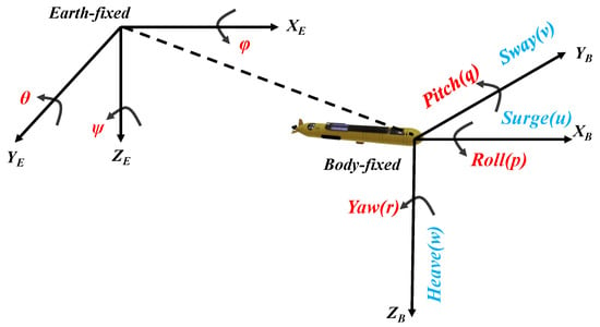
Figure 1.
Inertial and motion coordinate system of autonomous underwater vehicles (AUVs), the left is the Earth-fixed coordinate system, the right is the Body-fixed coordinate system.
The position state of the AUV vector is described by , where the position vector is used to describe the absolute position and attitude angle [21], which are termed surge, sway, heave, roll, pitch, and yaw, respectively. The velocity vector represents the three-axis linear velocity and the three-axis angular velocity in the body coordinate system. The kinematic relationship between the body coordinate system and the inertial coordinate system of the underwater AUV is
The above two vectors can be transformed into each other, and the transformation formula of the velocity vector of the motion in a two-coordinate system is as follows:
The attitude vector can be expressed as follows:
where
2.3. AUV Vertical Plane Control Description
To simplify the system model, we consider only the motion of the AUV platform in the vertical-axis model and the relationship between the world frame state and body frame state .
The motion state variables can be defined as , where u is the speed of the x-axis in the horizontal direction, z is the depth position, w is the velocity in the z-axis direction, is the pitch attitude angle, and q is the pitch attitude angular velocity. The motion relationship can be described by Equation (12):
The equation below describes the relationship between the linearized dynamic equation and the linearized external force and moment,
where and are linear drag coefficients, and are outside drivers, and are added mass matrices, is the mass moment of inertia about the y axis, and the other parameters are the same as before. Among the above variables, those that can be measured by the outside world are only x, z, and . Therefore, the complete AUV dynamic model in the form of state space equations is
where A is the state space matrix, B is the control matrix, and C is the output matrix. All the state space parameters can be described in detail as Equations (15) and (16). Here, the parameters , and all the AUV system parameters are shown in Table 1. Due to materials and assembly, the parameters of the system may change, and the intuitive indicator is the mass, which leads to the changes of the system model. From Equation (15), we can find that if the mass changed, the state space model of the AUV system will be changed. The open loop system’s matrices variables A, B, and C can be given, and the state space equation can be written as Equation (17).

Table 1.
Parameters of the AUV.
2.4. DRL Algorithm TD3 Description
DRL aims to discuss how agents can maximize their rewards in complex and uncertain environments. Reinforcement learning consists of agents and the environment interacting continuously during the learning process [16]. In this section, the DRL framework controls the errors between the actual system and reference model to converge the deviation to zero. Because the AUV system is a continuous control system, and various control variables are continuous, this study uses the strategic gradient algorithm for control. Both TD3 and the DDPG algorithms are typical applications of the strategic gradient algorithm, and the TD3 algorithm is a modified version of the DDPG algorithm. Because a comparison of the two is required later, only the difference between the two, that is, the improvement of TD3 is introduced here.
The TD3 algorithm, as a gradient policy with actor–critic, was used to solve the problem of Q overestimation, in which the following essential methods were adopted. First, the delayed update strategy function method was adopted to solve the coupling problem between the valuation function critic and actor policy functions. Second, the actor network was updated only once, whereas the critic network was updated every n times. The target network was then used to reduce the accumulation of errors, reduce variance reduction, and calculate the Q value, adding less noise to the action. The high variance build-up and the loss function are given by,
If mod d, then
where denotes the replay buffer, represents random noise, d denotes the policy frequency, and denotes the immediate reward r.
It is easy to overestimate the Q value because is used to replace and evaluate . In TD3, two sets of networks were used to estimate the Q value, where the smaller one is used as the update target. When a value function is updated, a minor disturbance is added to the input action each time. This operation is a target policy smoothing regulation. Policy noise was added to the target network when a parameter became available to make the assessment more accurate. TD3 is a deterministic policy algorithm, and the policy gradient function is
3. Proposed Method
The kinematics model was introduced in detail in Section 2. In this section, we introduce the implementation of acquiring the reference model from the basic kinematic model. In this study, to simplify the control model, the higher-order term near the working point was ignored. We can approximate the linear model equation in Section 3.1.1. We show the design process of the state space, action space, and reward function. Thereafter, the reference model was combined with the TD3 agent to formalize the MR-TD3 controller. From the perspective of the control theory, the architecture of the control system is shown in the block diagram in Figure 2, and each component is described in the following sections.
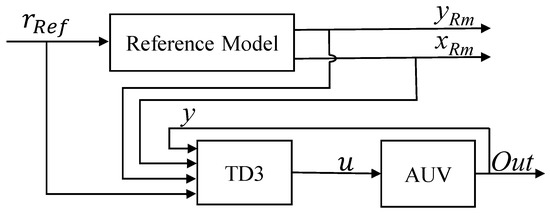
Figure 2.
Schematic of the control system; this framework is built from control theory perspective.
3.1. Control Method
Considering the nonlinearity and strong coupling of the system, a DRL neural network plays a critical role. The controller’s ability to prevent saturation and eliminate overshoot is also vital, and the part of the reference model serves as a baseline to guide the controlled target forward, thus smoothing the target to avoid an excessive overshoot. The maximum control command interval was considered in the design process of the reference model, which can prevent command control saturation and thus leave a control margin for external disturbances. Suppose that the target of the controller is a direct input target. This variable will be massive, which will cause the corresponding control variable to be relatively large, thus reaching the upper limit of the controller actuator. If there is any disturbance at this time, there will be no redundant control commands to deal with interference, and the robustness will be very poor. The role of the reference model was to track the target of the input. The parameters of the reference model can adjust the response time, and the output contains all observed variables, which is the derivation of the target and the reference target. The deviations between these values are relatively small, and the goal of the controller was to drive the deviation to zero.
3.1.1. Design of the Reference Model
Since the pitch and depth are a pair of coupling values in the underdriven system, the coupling quantities of the two channels are removed in the process of designing the reference model; that is, the coupling quantities can be regarded as external disturbances and removed to avoid the disturbance of the coupling quantities. So, the AUV system model without coupled values can be written as follow state space equation
A reference model was designed, whose output was the reference target variable that corresponded to the physical meaning of the input target variable. The reference model of the corresponding AUV system was designed according to the state space Equations (14)–(16)
Here, r is the reference input target, where , is set, and the state variable deviation can be calculated using the above formula,
We make the system satisfy the following conditions:
such that,
To ensure that output tracks the target variable r, the DC gain should be adjusted to one. Assuming infinite time, we drive the following formula
Output can be expressed as,
such that
and
The parameter can be adjusted using Matlab.
3.1.2. Simulation of the Reference Model
After adjustment and verification, considering both the response time of the reference model output value to the actual target and the constraints of the first-order derivation and control command of the mechanism in the actual system, the reference model state matrix and the control matrix can be written as follows:
The reference model’s depth and pitch step response are shown in Figure 3, where the depth response time is 30 s without overshoot, the maximum first-order derivative dive velocity w is m/s, and the peak second-order reference derivative dive acceleration is m/s, because when the command is full, the maximum acceleration is m/s. This indicated that in the tracking process, no matter what happend, the control command will not reach the saturation zone, because the reference model state is the biggest controlled value in this process. At the same time, pitch , as the other channel, is the indicator to be referred to for step response. The maximum pitch is rad, the response time is about 25 s, the maximum angular velocity is rad/s, and the maximum pitch acceleration is rad/s, which is also within the range of the actuator. Both of them are in the acceptable domain and will not get into the input saturation zone.
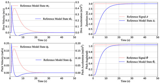
Figure 3.
Depth step response of the reference model. The SI unit on the x-axis is s, and for the y-axis, the units are m/s (left up), rad/s (left down), m (right up) and rad (right down), respectively.
3.2. Neural Network Approximators
Just as described in Section 2.4, we construct a three-layer neural network to train the AUV system. The evaluation network has 12 states as the input, and there are three driver commands as the output commands.
The control strategy consists of three layers of the neural network: the input state quantity is s, and the output control quantity is u. Due to the limitation and constraint of the control quantity range of the actual AUV system, the output control quantity must be controlled within the actual range, so the tanh unit is chosen as the output activation layer, and the output range after activation is , based on which the actual extuator range is scaled up and down. The hidden layer is also an important layer of the neural network, so the ReLu unit is chosen as the activation function of the hidden layer. The final structure of the neural network is shown in Figure 4.
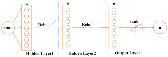
Figure 4.
The structure of the policy network, which consists of three layers: the hidden layer action unit is Relu, and the output layer action unit is tanh.
3.3. Integrated Controller of MR-TD3
In this study, an AUV control system with a reference model-based controller is proposed in Section 3.1. The DRL agent TD3 is described in Section 2.4, where the reference signal was generated according to the control objective, the AUV system was analyzed, and the position, surge velocity, depth, dive velocity, pitch angle, and angular velocity were selected as the control variables. The errors are used as the state variables to form the reference model of the AUV system. Because our proposed controller consists of the TD3 algorithm and the model reference control method, it is termed the MR-TD3 controller, and the block diagram of MR-TD3 is shown in Figure 5.
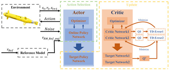
Figure 5.
MR-TD3 controller structure; this framework is built in DRL perspective.
In reinforcement learning, such as pendulum, the reward function includes the angle, angular velocity, and control volume, which does not consider the longtime command range. In contrast, for the AUV control system, we should consider not only the absolute error of the system but also the response time, overshoot, and actuator command scope. There are many types of AUV system states, such as depth, velocity, acceleration, attitude, angle, angular velocity, and angular acceleration. The AUV control system should consider both the response time and system stability. From the controller principle structure in Figure 2 and the DRL agent shown in Figure 5, we can see that the input state consists of the state of the reference model and the reference target variable. Therefore, the reward function is designed in the following form in Figure 2 and Figure 5; one is represented by the block diagram of the control system and the other is represented by the block diagram of reinforcement learning. Both names are slightly different, but the meanings are the same.
where is the output of the reference model, y is the output of the actual controlled object, is the observed state output of the reference model, and u is the control command, in the DRL agent, that is, the output action of TD3. In the system control process, there is an intuitive understanding that the less energy consumed, the better. Therefore, a reward function is established for the power that directly corresponds to the control value u to make the system controller move toward the target direction and avoid spinning in place.
The coefficients of all the reward variables are .
3.4. Flowchart and Pseudocode
Unlike stochastic strategies, deterministic strategies require additional control variables as opposed to a random exploration of state actions. Our approach was to add noise to the action output, and the actuator range determined the max command value of the action.
where represents normally distributed noise . The actor–critic network structure of MR-TD3 is shown in Figure 5. When optimizing the evaluation network, the goal of the gradient strategy is no longer to track the target angle but to keep the state of the AUV close to the output state of the reference model, which avoids saturation of the control commands. The reference model state vector was used for pitch control, whereas was used for depth control. The neural network structure was designed according to the actor–critic and TD3 structures [11].
The control objective of MR-TD3 was to optimize the control volume output with an action layer of three, a state layer of twelve, and a hidden layer of 256 × 256. In AUV control applications, the actions must be restricted in the reinforcement learning action space; that is, the agent control instructions are within the action space of the execution structure. In practical applications, a sigmoid function was used at the output level to restrict the control signal to a reasonable range and to introduce deviations into the AUV controller. The purpose of this approach is to let the error integral be considered as the control input to the policy network. The actor–network input includes the AUV reference model state, the actual AUV state, and the integration error, and the critic network input is the action of the actor output. During the optimal evaluation of the network, the goal of the gradient strategy is no longer to track the target angle but to make the AUV output state follow the output state value of the reference model, and this process eliminates the saturation of the control commands.
The MR-TD3 algorithm was designed in episode mode. First, the parameters of the critic network were cloned as the target critic network whereafter the state was initialized. Each state must be within a suitable range, and all state transition models were stored in the replay buffer. When the buffer storage capacity was sufficient, the minimum min-batch was collected and the training process was initiated. The algorithm flow is shown in Algorithm 1.
| Algorithm 1 MR-TD3 for the Depth and Pitch controller of the AUV |
|
4. Computational Experiment
In this section, we set the specific parameters of the selected model and state parameters of the controller designed above. Thereafter, we simulated the set target values, compared the performance in various experiments, and finally analyzed and discussed their performance.
4.1. Experimental Setting
We selected an AUV model to simulate the performance of the proposed algorithms. All model parameters are listed in Table 1 [37].
The experimental hardware is an 11th Gen Intel(R) Core(TM) i9-11900H @ 2.50 GHz and the operating system is Ubuntu18.04. The network was developed by Python with pytorch. In the training process, we use Adam optimizer, so there is no GPU or parallel computing technique needed in our experiments.
The linear system model follows Equation (17); the DRL neural network and training parameters are shown in Table 2.
Table 2.
Parameters of Training.
4.2. Training Result
The strategy gradient optimization algorithm is described in Section 2.4. Because TD3 adds a dual critic and actor network to DDPG, it solves the problem of overestimation of Q values, delays the update of actors, stabilizes the training process, and adds noise to the output of the target network of actors. Thus, the proposed algorithm was more stable.
From the reward curve in Figure 6, the green curve is the MR-TD3 algorithm and the red curve is the MR-DDPG algorithm. In the curve of MR-TD3, the peak variance is reached first, and it is stable, whereas DDPG is overestimated and dramatically fluctuates during the run process. These behaviors are the same in the case of the MR-DDPG training process, which is consistent with the characteristics of DDPG, and it can also be seen that the TD3 is better trained. During this process, the training process was not stabilized. However, the difference between MR-DDPG and MR-TD3 is not very large, and both are relatively good DRL algorithms.
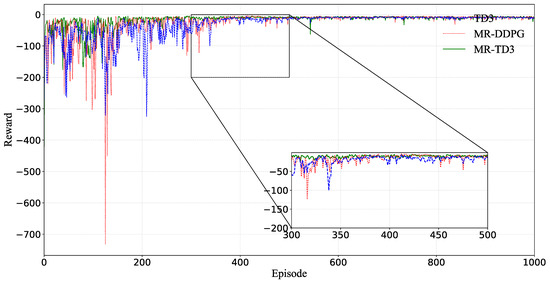
Figure 6.
Training reward for TD3, MR–DDPG and MR–TD3. The x-axis is the episode and the y-axis is the reward of each episode. The magnification area is from the 300th to the 500th episode, and the y-axis range is between −200 and 0.
4.3. Simulation Result
In this section, we test the performance of the depth and pitch controllers and discuss all these simulation results. The experiments consisted of the following parts: Firstly, the TD3 and MR-TD3 controllers were used to control the depth and pitch angle, respectively, as well as verify the effect of the reference model on the control volume overshoot and actuator saturation. Secondly, the mass and the initial position of the AUV was adjusted to confirm that the designed controller is robust.
4.3.1. Depth Response and Overshoot Experimental Result
In the field of AUV control, the response time and overshoot are the two primary performance indicators of the controller. To test the performance of the DRL controller, we designed comparative experiments with TD3 and proposed the MR-TD3 method to discuss the step response and sine wave response. For the pitch channel, the target is the attitude angle and attitude angular velocity; the command of elevator rudder control should be concerned as the process reference value. For the depth channel, the target was the depth, and the process reference values were the diving speed and corresponding control commands. The depth and pitch angle are a pair of coupled values; these two can affect each other, so all the process variables of pitch and depth must be observed during the control process. In these experiments, the surge velocity is a fixed value of 2 m/s.
We first test the depth step response and sine response, in which all the initial state is zero, the step target depth is m, the sinusoidal amplitude target is 1 m, and the deviation of the sine curve is positive one. Figure 7 illustrates the states of the depth step response and sine wave response of the AUV system and the control command of the two channels.
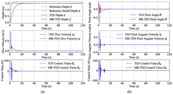
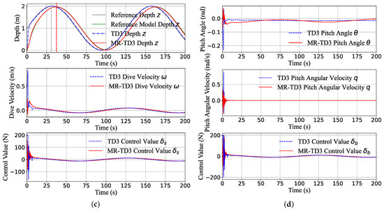
Figure 7.
The depth channel transition of the system states (z-position, dive velocity, pitch angle and pitch angular velocity) and control command during the step response (a,b) and sine wave response (c,d). The maximum actuator command is 200 N. It can be seen that the TD3 method tends to provide a full control command, which is unacceptable in real machines. In contrast, the MR-TD3 command is smoother and can eliminate the overshoot significantly.
In Figure 7a,b, the classical TD3 agent always tends to choose the maximum control command to follow the target, the maximum depth reaches 1.6 m (overshoot about ) in 5 s, and the elevator rudder comes into the full command 200 N and stays in this zone about 3 s, just as for the MR-TD3 agent. Because the reference target is not changed dramatically to m, the MR-TD3 command can smoothly follow the reference model depth target and reach the reference depth in 30 s; this time is the same as shown in Figure 3. However, since the ultimate control object is depth, not the reference model depth, upon comparing the two algorithms, just as Figure 8 shows, we can find that at the start time, the deviation of the two algorithms is 1.5 m, but the TD3 agent can drive the error to zero quickly in 4 s and the MR-TD3 agent can drive the error to zero in 30 s. To make it easier to compare the two results, the response time and overshoot are listed in Table 3. As the first-order derivative of depth control, the TD3 agent’s peak velocity of the depth step response is almost 1 m/s; this is almost three times that of the MR-TD3 agent. In addition, the second-level cascade system, pitch angle , angular velocity q and the corresponding control command, as seen in Figure 7b, have the same response time and depth control trend.
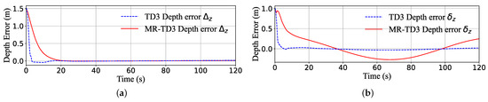
Figure 8.
The depth channel response error of the TD3 and MR-TD3 agent. The error is the deviation between the reference target value and the actual agent response value. The step depth response is (a) and the sine depth response is (b).
Table 3.
Comparison of response time and overshoot in depth channel.
Figure 7c,d are the depth sine response result. The TD3 agent can generate full command at 200 N and keeps about 4 s; this can track the reference depth in about 6 s, and then, the command can be changed to follow the target value. However, as for the MR-TD3 agent, the command can track the reference model value tightly, but it is always 5 s slower than the reference depth value.
- (1).
- In a step test scenario, the TD3 agent has a better response time but the MR-TD3 agent has better overshoot capacity.
- (2).
- In a sine test scenario, the MR-TD3 agent always has a 5 s delayed reaction.
- (3).
- The response time of the MR-TD3 agent is the same as that of the reference model.
4.3.2. Pitch Response and Overshoot Experimental Result
Figure 9 illustrates the pitch step response and pitch sine wave response of the two methods, in which all the initial state is , the sinusoidal amplitude target is 0.75 , and the deviation of the sine curve is positive.
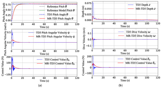
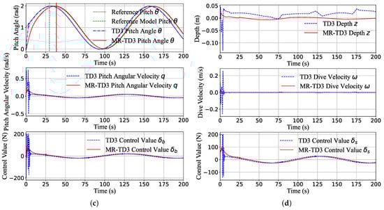
Figure 9.
The pitch channel transition of the system states (pitch angle, pitch angular velocity, z-position, dive velocity) and control command during the step response (a,b) and sine wave response (c,d). The maximum actuator command is 200 N; it can be seen that the TD3 method tends to provide a full control command, which is unacceptable in real machines. In contrast, the MR-TD3 command is smoother and can eliminate the overshoot significantly.
We can see that TD3 algorithms always tend to choose the maximum control command to track the target as close as possible; the tracking speed is so fast that the pitch angular velocity can reach rad/s in 1 s, and the pitch can reach the peak in about 3 s and has a overshoot but becomes stable at nearly 10 s (Figure 9a). Although the pitch control command did not reach the full zone, the depth control command reached the peak command 200 N for about 5 s (Figure 9b). The MR-TD3 agent can reach the target pitch in 25 s, and all the transition states are very smooth. Figure 9c,d are the pitch sine response simulation, which is almost the same as the depth sine response, the TD3 agent response time is 4 s, and MR-TD3 always has a nearly 7 s delay response behind the reference target.
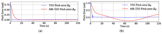
Figure 10.
The pitch channel response error of TD3 and the MR-TD3 agent. The error is the deviation between the reference target value and the actual agent response value. The step pitch response is (a) and the sine pitch response is (b).
Table 4.
Comparison of the response time and overshoot in pitch channel.
- (1).
- In the pitch step test scenario, the TD3 agent has better response time but MR-TD3 is smoother.
- (2).
- In the pitch sine test scenario, the MR-TD3 agent always has a 7 s delayed reaction.
- (3).
- The response time of MR-TD3 is the same as that of the reference model.
4.3.3. Analysis
From Figure 7 and Figure 9, during the training process, to track the target, the actor of DRL will keep accumulating rewards, and faster tracking will lead to more rewards, so the TD3 method easily enters the saturation domain. It can also be seen that the response speed of the TD3 controller is faster than that of the MR-TD3 controller. This result is acceptable in the simulation process. Still, in the actual application, this control command is strong enough to follow the target as closely as possible. The control command will reach the maximum value (command saturation). Any external noise will lead to oscillation and instability, and the long-time control command saturation will also lead to the actuator overheating and damage. In contrast, the MR-TD3 controller chooses the reference target as the guide baseline instead of tracking the target directly, and the reference baseline will make a balance between the response time and the maximum control command.
The above figures also verify the first contribution proposed in this study, where the DRL agent of the MR-TD3 controller relative to the direct control can constrain the control commands to avoid the overshoot of the actuator and thus enter the saturation space.
The depth and pitch step response time of MR-TD3 are 30 s and 25 s, respectively, just in Table 3 and Table 4; this is the same as that in Figure 3. This phenomenon shows that the response time of the reference model control is determined by the parameters of the reference model, and it also proved the importance of the model parameters selection; these ultimately determine MR-TD3’s performance.
From Figure 7, Figure 8, Figure 9 and Figure 10 and Table 3 and Table 4, in the TD3 method, when the controlled object is the depth, the pitch angle and depth are a pair of coupling quantities. The response time of the pitch angle (25 s) is shorter than the depth (30 s) due to the cascading system and maintaining the rolling balance of the system. In the MR-TD3 method, as these two have been decoupled in the reference model, according to the actual intermediate state quantity of the system, that is, the dive velocity and pitch angular velocity, the pitch response time of the reference model is less than that of the depth. The above can be summarized as:
- (1).
- The TD3 agent has better response time but has overshoot.
- (2).
- The MR-TD3 state is much more smoother; all the commands will not reach the saturation zone, and there is a fixed delay reaction in the sine test.
- (3).
- The MR-TD3 response time is the same as that of the reference model.
- (4).
- As cascading AUV systems, pitch is the first level and depth is the second level; pitch always has a faster response than depth.
4.3.4. Robust Test of MR-TD3 Controller
This section tests the robustness of the trained agent. The purpose of the test is to change some initial state of the controlled object and check whether the controller can still keep the object stable.
- (1)
- Case I: Model Generalization.
From Equation (15), it is most convenient to change the mass m of the system to change the AUV model. Therefore, the weight of the AUV system is altered here to perform the robust test. The task is the robustness step response test of the MR-TD3 controller for the depth with initial position 0 m to reference position m. We changed the mass of the AUV system by decreasing it by ( (kg)) and (kg)) and then increasing it by (kg)), (kg)) and (kg)), while all the other parameters remain the same. From Figure 11, we can observe that the controller remained stable when the weight changed within .
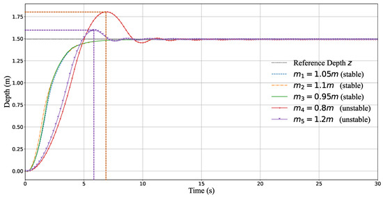
Figure 11.
Depth robust step response of MR-TD3. The controller is robust to different masses of the AUV to maintain a consistent depth performance.
However, for the AUV system with a weight decrease, the peak overshoot (about ) of the depth is m at the time of the 7 s, and the phenomenon of oscillation appears again until about the 15 s. Correspondingly, when the mass was increased, the peak overshoot (about ) appears at the time of the 6 s. We consider this experimental result reasonable because the disturbance or robustness must be a small proportion compared to the control value. If the percentage is too large compared with the control amount and dominates, the controller must be redesigned.
- (2)
- Case : Random Initial State
Furthermore, we test whether the MR-TD3 controller can stabilize the AUV system with different initial positions. The control object is used to drive the AUV from a different initial depth back to 2 m; the other states and parameters are kept unchanged, each episode lasts for 10 s, and the MR-TD3 agent convged all the states to 2 m in 6 s. Figure 12 verifies that the proposed controller has the stability to drive the AUV to the target depth smoothly.
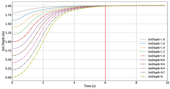
Figure 12.
Depth robust step response of MR-TD3; the MR-TD3 controller can drive the AUV system to the stable status from different initial depth positions.
- (3)
- ConclusionFrom the above two cases, we can come to the conclusion that:
- (1).
- MR-TD3 has the capacity of robustness, but the controlled object can only be changed by 10%.
- (2).
- MR-TD3 can converge from different initial positions, and the converge time is the same.
5. Conclusions
This study proposed a new control algorithm, the MR-TD3 algorithm, for controlling AUV systems. We analyzed the system model and set up the state space equation of the AUV system. Thereafter, we designed the reference model and system state variables to follow the target. Finally, we conducted pitch and depth control experiments using MR-TD3 and TD3 controllers to test the response time and overshoot performance.
The results show that the MR-TD3 algorithm can reduce the overshoot of control commands and eliminate the saturation of control commands. This can maintain the stability and anti-disturbance ability of the system. Moreover, this algorithm combines reinforcement learning with a reference model to provide a robust and applicable control method.
However, we also found that the reference model had a significant impact on the saturation and robustness of the instructions, indicating that the parameters of the reference model response time and the control magnitude play a crucial role. Additionally, these parameters may lead to a lack of robustness, thus leading to the control instruction of system saturation being made again. On the other hand, the designed MR-TD3 algorithm improves the saturation and robustness of the instructions but at the expense of the response speed, which is an issue to be considered in future research. In future work, we hope to solve the problem of response time and test the method in an actual platform. We also hoped that the method can be used in other control scenarios, such as autonomous guided vehicles and UAV.
Author Contributions
Conceptualization, J.D.; methodology, J.D. and S.A.; software, D.Z. and J.D.; validation, J.D.; formal analysis, J.D.; investigation, J.D.; resources, J.D.; data curation, J.D.; writing—original draft preparation, D.Z. and J.D.; writing—review and editing, S.A., W.W.; visualization, J.D.; supervision, S.A. All authors have read and agreed to the published version of the manuscript.
Funding
This research received no external funding.
Institutional Review Board Statement
Not applicable.
Informed Consent Statement
Not applicable.
Data Availability Statement
Not applicable.
Conflicts of Interest
The authors declare no conflict of interest.
Abbreviations
The following abbreviations are used in this manuscript:
| MDPI | Multidisciplinary Digital Publishing Institute |
| DOAJ | Directory of open access journals |
| TLA | Three-letter acronym |
| LD | Linear dichroism |
| AUV | Autonomous Underwater Vehicle |
| DRL | Deep Reinforcement Learning |
| MR-TD3 | Model-Reference Twin Delayed Deep Deterministic |
| TD3 | Twin Delayed Deep Deterministic |
| AUVs | Autonomous Underwater Vehicles |
| MIMO | Multi-Input–Multi-Output |
| DQN | Deep Q-learning Network |
| PPO | Proximal Policy Optimization |
| UAV | Unmanned Aerial Vehicle |
| NMPC | Nolinear Model Predictive Control |
| LQG | Linear–Quadratic–Gaussian |
| NED-Frame | North–East–Down Frame |
| DOF | Degree-of-Freedom |
| 6DOF | Six Degrees-of-Freedom |
| 3DOF | Three Degrees-of-Freedom |
| NED-Frame | North–East–Down Frame |
References
- Blidberg, D.R. The Development of Autonomous Underwater Vehicles (AUV); A Brief Summary. In Proceedings of the IEEE International Conference on Robotics and Automation, Seoul, Republic of Korea, 21–26 May 2001; Volume 4, pp. 1–12. [Google Scholar]
- Amran, I.Y.; Kadir, H.A.; Ambar, R.; Ibrahim, N.S.; Kadir, A.A.A.; Mangshor, M.H.A. Development of autonomous underwater vehicle for water quality measurement application. In Proceedings of the 11th National Technical Seminar on Unmanned System Technology 2019: NUSYS’19, Singapore, 2–3 December 2019; pp. 139–161. [Google Scholar]
- Fossen, T.I. Handbook of Marine Craft Hydrodynamics and Motion Control; John Wiley & Sons: New York, NY, USA, 2011. [Google Scholar]
- Miao, J.; Wang, S.; Zhao, Z.; Li, Y.; Tomovic, M.M. Spatial curvilinear path following control of underactuated AUV with multiple uncertainties. ISA Trans. 2017, 67, 107–130. [Google Scholar] [CrossRef]
- Sutton, R.S.; Barto, A.G. Reinforcement Learning: An Introduction; MIT Press: Cambridge, MA, USA, 2018. [Google Scholar]
- Mnih, V.; Kavukcuoglu, K.; Silver, D.; Rusu, A.A.; Veness, J.; Bellemare, M.G.; Graves, A.; Riedmiller, M.; Fidjeland, A.K.; Ostrovski, G.; et al. Human-level control through deep reinforcement learning. Nature 2015, 518, 529–533. [Google Scholar] [CrossRef] [PubMed]
- Lillicrap, T.P.; Hunt, J.J.; Pritzel, A.; Heess, N.; Erez, T.; Tassa, Y.; Silver, D.; Wierstra, D. Continuous control with deep reinforcement learning. arXiv 2015, arXiv:1509.02971. [Google Scholar]
- Mnih, V.; Kavukcuoglu, K.; Silver, D.; Graves, A.; Antonoglou, I.; Wierstra, D.; Riedmiller, M. Playing Atari with Deep Reinforcement Learning. arXiv 2013, arXiv:1312.5602. [Google Scholar]
- Schulman, J.; Wolski, F.; Dhariwal, P.; Radford, A.; Klimov, O. Proximal Policy Optimization Algorithms. arXiv 2017, arXiv:1707.06347. [Google Scholar]
- Haarnoja, T.; Zhou, A.; Hartikainen, K.; Tucker, G.; Ha, S.; Tan, J.; Kumar, V.; Zhu, H.; Gupta, A.; Abbeel, P.; et al. Soft Actor-Critic Algorithms and Applications. arXiv 2018, arXiv:1812.05905. [Google Scholar]
- Fujimoto, S.; Hoof, H.V.; Meger, D. Addressing Function Approximation Error in Actor-Critic Methods. In Proceedings of the International Conference on Machine Learning, Stockholm, Sweden, 10–15 July 2018. [Google Scholar]
- Fang, Y.; Pu, J.; Zhou, H.; Liu, S.; Cao, Y.; Liang, Y. Attitude control based autonomous underwater vehicle multi-mission motion control with deep reinforcement learning. In Proceedings of the 2021 5th International Conference on Automation, Control and Robots (ICACR), Nanning, China, 25–27 September 2021; pp. 120–129. [Google Scholar]
- Jiang, J.; Zhang, R.; Fang, Y.; Wang, X. Research on motion attitude control of under-actuated autonomous underwater vehicle based on deep reinforcement learning. J. Phys. Conf. Ser. 2020, 1693, 012206. [Google Scholar] [CrossRef]
- Koch, W.; Mancuso, R.; West, R.; Bestavros, A. Reinforcement Learning for UAV Attitude Control. ACM Trans. Cyber-Phys. Syst. 2019, 3, 1–21. [Google Scholar] [CrossRef]
- Liu, H.; Suzuki, S.; Wang, W.; Liu, H.; Wang, Q. Robust Control Strategy for Quadrotor Drone Using Reference Model-Based Deep Deterministic Policy Gradient. Drones 2022, 6, 251. [Google Scholar] [CrossRef]
- Wu, H.; Song, S.; You, K.; Wu, C. Depth Control of Model-Free AUVs via Reinforcement Learning. IEEE Trans. Syst. Man, Cybern. Syst. 2018, 49, 2499–2510. [Google Scholar] [CrossRef]
- Liu, Y.; Wang, M.; Su, Z.; Luo, J.; Xie, S.; Peng, Y.; Pu, H.; Xie, J.; Zhou, R. Multi-AUVs Cooperative Target Search Based on Autonomous Cooperative Search Learning Algorithm. J. Mar. Sci. Eng. 2020, 8, 843. [Google Scholar] [CrossRef]
- Sands, T. Development of Deterministic Artificial Intelligence for Unmanned Underwater Vehicles (UUV). J. Mar. Sci. Eng. 2020, 8, 578. [Google Scholar] [CrossRef]
- Koo, S.M.; Travis, H.; Sands, T. Impacts of Discretization and Numerical Propagation on the Ability to Follow Challenging Square Wave Commands. J. Mar. Sci. Eng. 2022, 10, 419. [Google Scholar] [CrossRef]
- Zhai, H.; Sands, T. Comparison of Deep Learning and Deterministic Algorithms for Control Modeling. Sensors 2022, 22, 6362. [Google Scholar] [CrossRef]
- Guo, X.; Yan, W.; Cui, R. Integral Reinforcement Learning-Based Adaptive NN Control for Continuous-Time Nonlinear MIMO Systems With Unknown Control Directions. IEEE Trans. Syst. Man Cybern. Syst. 2019, 50, 4068–4077. [Google Scholar] [CrossRef]
- Bøhn, E.; Coates, E.M.; Moe, S.; Johansen, T.A. Deep reinforcement learning attitude control of fixed-wing uavs using proximal policy optimization. In Proceedings of the 2019 International Conference on Unmanned Aircraft Systems (ICUAS), Atlanta, GA, USA, 11–14 June 2019; pp. 523–533. [Google Scholar]
- Huang, F.; Xu, J.; Yin, L.; Wu, D.; Cui, Y.; Yan, Z.; Chen, T. A general motion control architecture for an autonomous underwater vehicle with actuator faults and unknown disturbances through deep reinforcement learning. Ocean Eng. 2022, 263, 112424. [Google Scholar] [CrossRef]
- Arora, S.; Doshi, P. A survey of inverse reinforcement learning: Challenges, methods and progress. Artif. Intell. 2021, 297, 103500. [Google Scholar] [CrossRef]
- Vu, M.T.; Le, T.H.; Thanh, H.L.N.N.; Huynh, T.T.; Van, M.; Hoang, Q.D.; Do, T.D. Robust position control of an over-actuated underwater vehicle under model uncertainties and ocean current effects using dynamic sliding mode surface and optimal allocation control. Sensors 2021, 21, 747. [Google Scholar] [CrossRef] [PubMed]
- Vu, M.T.; Le Thanh, H.N.N.; Huynh, T.T.; Thang, Q.; Duc, T.; Hoang, Q.D.; Le, T.H. Station-Keeping Control of a Hovering Over-Actuated Autonomous Underwater Vehicle Under Ocean Current Effects and Model Uncertainties in Horizontal Plane. IEEE Access 2021, 9, 6855–6867. [Google Scholar] [CrossRef]
- Nguyen, N.T. Model-reference adaptive control. In Model-Reference Adaptive Control; Springer: Cham, Switzerland, 2018; pp. 83–123. [Google Scholar]
- Parks, P. Liapunov redesign of model reference adaptive control systems. IEEE Trans. Autom. Control 1966, 11, 362–367. [Google Scholar] [CrossRef]
- Kreisselmeier, G.; Anderson, B. Robust model reference adaptive control. IEEE Trans. Autom. Control 1986, 31, 127–133. [Google Scholar] [CrossRef]
- Li, J.H.; Lee, P. Design of an adaptive nonlinear controller for depth control of an autonomous underwater vehicle. Ocean Eng. 2005, 32, 2165–2181. [Google Scholar] [CrossRef]
- Sarhadi, P.; Noei, A.R.; Khosravi, A. Adaptive integral feedback controller for pitch and yaw channels of an AUV with actuator saturations. Isa Trans. 2016, 65, 284–295. [Google Scholar] [CrossRef]
- Nicholas, L.T.; Valladarez, D.; Du Toit, N.E. Robust adaptive control of underwater vehicles for precision operations. In Proceedings of the OCEANS 2015-MTS/IEEE Washington, Washington, DC, USA, 19–22 October 2015; pp. 1–7. [Google Scholar]
- Sarhadi, P.; Noei, A.R.; Khosravi, A. Model reference adaptive PID control with anti-windup compensator for an autonomous underwater vehicle. Robot. Auton. Syst. 2016, 83, 87–93. [Google Scholar] [CrossRef]
- Makavita, C.D.; Nguyen, H.D.; Ranmuthugala, D.; Jayasinghe, S.G. Composite model reference adaptive control for an uncrewed underwater vehicle. Underw. Technol. 2015, 33, 81–93. [Google Scholar] [CrossRef]
- Zuo, M.; Wang, G.; Xiao, Y.; Xiang, G. A Unified Approach for Underwater Homing and Docking of over-Actuated AUV. J. Mar. Sci. Eng. 2021, 9, 884. [Google Scholar] [CrossRef]
- Vu, M.T.; Van, M.; Bui, D.H.P.; Do, Q.T.; Huynh, T.T.; Lee, S.D.; Choi, H.S. Study on dynamic behavior of unmanned surface vehicle-linked unmanned underwater vehicle system for underwater exploration. Sensors 2020, 20, 1329. [Google Scholar] [CrossRef] [PubMed]
- Packard, G.E.; Kukulya, A.; Austin, T.; Dennett, M.; Littlefield, R.; Packard, G.; Purcell, M.; Stokey, R. Continuous autonomous tracking and imaging of white sharks and basking sharks using a REMUS-100 AUV. In Proceedings of the 2013 OCEANS-San Diego, San Diego, CA, USA, 23–27 September 2013. [Google Scholar]
- Prestero, T. Verification of a Six-Degree of Freedom Simulation Model for the REMUS Autonomous Underwater Vehicle. Doctoral Dissertation, Massachusetts Institute of Technology, Cambridge, MA, USA, 2001. [Google Scholar]
- Society of Naval Architects and Marine Engineers (U.S.). Technical and Research Committee. Hydrodynamics Subcommittee. In Nomenclature for Treating the Motion of a Submerged Body Through a Fluid: Report of the American Towing Tank Conference; Society of Naval Architects and Marine Engineers: Alexandria, VA, USA, 1950; pp. 1–15. [Google Scholar]
- Naus, K.; Piskur, P. Applying the Geodetic Adjustment Method for Positioning in Relation to the Swarm Leader of Underwater Vehicles Based on Course, Speed, and Distance Measurements. Energies 2022, 15, 8472. [Google Scholar] [CrossRef]


Disclaimer/Publisher’s Note: The statements, opinions and data contained in all publications are solely those of the individual author(s) and contributor(s) and not of MDPI and/or the editor(s). MDPI and/or the editor(s) disclaim responsibility for any injury to people or property resulting from any ideas, methods, instructions or products referred to in the content. |
© 2023 by the authors. Licensee MDPI, Basel, Switzerland. This article is an open access article distributed under the terms and conditions of the Creative Commons Attribution (CC BY) license (https://creativecommons.org/licenses/by/4.0/).