Wave Runup Prediction and Alongshore Variability on a Pocket Gravel Beach under Fetch-Limited Wave Conditions

Abstract

Most empirical equations used for wave runup predictions have been developed from measurements at straight sandy beaches in unlimited fetch environments. While there are empirical equations to predict wave runup on gravel beaches, they have not been tested for prediction of wave runup on pocket gravel beaches, in limited-fetch environment, which can be found around Mediterranean. This paper addresses this lack of measurements on this type of beaches and examines the alongshore variability of wave runup. Wave runup measurements were made using video observations along 3 cross-sectional profiles on the pocket beach of Ploče, Croatia. The measurements have shown that the wave runup can vary for about 71% even around the centerline of the pocket beach. This variability is due to beach orientation and alignment of beach profiles to the prevailing wave direction, as well as difference in beach slope. Comparison of wave runup predictions from five well-known empirical equations and field measurements showed significant underprediction (up to NBIAS = −0.33) for energetic wave events, and overall high scatter (up to NRMSE = 0.38). The best performing wave runup equation was used for further refinement outside the original parameter space by including the Goda wave peakedness parameter (Q_p). The newly developed empirical equation for wave runup reduced the NBIAS to 0 and the NRMSE by 31% compared to the original equation (developed equation metrics: R = 0.91, NBIAS = 0, NRMSE = 0.2, HH = 0.2 on the study site). This empirical equation can potentially be used for design of coastal structures and artificial beaches in similar environments, but further measurements are needed to test its applicability to a range of forcing and environmental conditions.

1. Introduction

Wave runup prediction is of great interest to coastal engineers and managers for the design of coastal structures. Wave runup is defined as the maximum elevation of the water uprush on the shoreline. However, most engineering applications commonly refer to the wave runup value exceeded by only 2% of the wave uprushes (R_2%), not the maximum wave runup (R_max). The main components of wave runup are wave setup and swash. Wave setup is generated by the wave breaking mechanism in the surf zone. During the wave breaking, one part of the wave energy is transferred as momentum to an additional elevation on the shoreline (quasi steady wave setup, <η>) [1]. On the other hand, the remaining wave energy reaches the shoreline and causes water oscillations (swash, S) [2]. Swash on a beach can be of higher frequencies, those of incident frequency band (0.05 Hz to 0.5 Hz) or at lower frequencies of infragravity frequency band (0.003 Hz to 0.05 Hz) [3,4]. During extreme storms, wave runup often coincides with high tides and high surge levels, which increase still water level, SWL, resulting in coastal flooding, berm overtopping, and significant morphological changes to the beachface [3,5,6,7,8,9].

Although the general mechanics of wave runup are understood, the entire process of energy transfer from offshore to the shoreline is highly nonlinear and has several parameters that are difficult to capture, such as the ever-changing beach profile. Commonly, wave run up predictions are made using empirical equations derived from laboratory and field measurements [10]. In recent years, numerical models are also used for simulation and prediction of wave runup. For example, phase-resolved numerical wave models (based on the Boussinesq equation models and/or non-linear shallow water equations) for a non-hydrostatic surface flow can be used [11,12]. Numerical models such as SWASH and FUNWAVE have been used to predict wave runup in laboratory and field conditions [13,14,15,16]. Some studies used numerical models (e.g., XBeach-G) to augment the wave runup observation in the laboratory or field [17]. Numerical modeling makes it easier to integrate complex beach layouts (e.g., barred and non-barred profiles), which could be difficult to integrate into a simple empirical expression [3]. It also allows to test a range of different forcing and beach conditions, which is difficult to simulate in laboratory experiments or measure in field. However, in field applications numerical model assumptions could be violated and boundary conditions poorly known [3,12]. Thus, empirical equations could be easier to use for wave runup prediction compared to numerical simulations [17,18,19], which is attractive for engineering applications. In empirical equations the runup is often correlated with wave and morphology parameters based on data from laboratory experiments [20,21,22] or field measurements [4,23,24,25,26,27,28]. Commonly used parameters are offshore significant wave height (H_s), peak wave period (T_p), wavelength (L₀) and beachface slope (β).

Primarily, the focus of field wave runup measurements has been on wave runup on sandy beaches with open coasts that are exposed to both sea and swell waves [3,17]. Some examples include studies by [4,25,27,29,30,31]. A well-known and widely used empirical equation was derived in the work of Stockdon, et al. [4].

Empirical equations, however, are limited to a specific range of environmental conditions that existed at the time the data were collected. Therefore, the application of equations for wave runup from large-fetch sandy beaches to fetch limited and/or gravel beaches is inappropriate. Predictions that fall outside the range of the data used to formulate the equations are then extrapolated, leading to significant uncertainties and potential errors. In particular if these equations are applied in environments with different types of beach morphology, such as complex topography and embayed beaches, due to sheltering effects [32,33,34,35]. For example, the well-known equation from Stockdon, et al. [4] was originally developed based on data from open sandy beaches in the United States and the Netherlands, so its suitability for other beach types is questionable.

Gravel beaches are considered a sustainable form of coastal protection during high tides and storms [36,37] and several studies focused on wave runup predictions for this type of beaches. On open gravel beaches, Poate, et al. [17] and Almeida, et al. [38] have already observed that wave runup reaches higher elevations in comparison to sandy beaches. They also found that predictions do not match with measurements when using equations for wave runup derived from sandy beaches. They attributed the observed difference between measurements and predictions to a steeper beach profile of gravel beaches that maintains a reflective beach behavior even under extremely energetic conditions by making adjustments to the beach step [39,40,41]. This was also found by Masselink, et al. [42], who tested the applicability of the equation by Stockdon, et al. [4] on several gravel beaches in the United Kingdom and concluded that wave runup under energetic wave conditions is significantly underestimated by the equation. Overall, pure gravel beaches consist of coarse sediment (D₅₀ of 3–75 mm), so the beaches generally have steep profiles (tanβ of about 0.1). Their behavior under energetic wave conditions is different; while sandy beaches are dominated by swash from the infragravity frequency band (0.003 Hz to 0.05 Hz), gravel beaches are dominated by swash from the incident frequency band (0.05 Hz to 0.5 Hz) [4,27,29,31,43,44].

Wave runup on fetch-limited beaches, on the other hand, is expected to be reduced, regardless of the beach sediment composition [45]. The reduction in wave runup is due to the sheltering effects that inhibit offshore swell and limit the space for local growth of wind waves. These fetch-limited beaches are typically characterized by low wave energy and short offshore wavelengths [3,46,47]. However, water levels can be significantly increased during rare but extreme events, not only by storm surges on the top of tidal levels but also in the form of wave setup and runup [33,48,49]. These wave effects can lead to flooding [50], the extent of which depends on the offshore wave climate and beach morphology [51]. So far, predictions of wave runup in these areas of low wave energy have received less attention [46,52,53].

So far, studies were mainly focused on straight uniform beaches and at a representative beach profile. However, beaches have often complex bathymetry that results in non-uniform wave setup and wave runup along the coast. Often, the dynamics of wave runup at different tidal stages on beaches with complex 3D morphology, is not fully understood [54,55]. For example, Guedes, et al. [56] observed that the alongshore variability in foreshore slope causes variability in wave runup on a dissipative beach, even when low complexity morphology (no beach cusps, rip currents, or crescentic bars) is considered. Senechal, et al. [44] studied the variation of wave runup in stationary storm waves under dissipative conditions in the presence of a shoreline sand wave. They concluded that a very complex beach morphology can lead to a spatial variation of wave runup by a factor of 3, which is mainly influenced by the morphology of the inner surf or, in other words, by the wave refraction around the sand wave. All these studies underline the enormous complexity of the 3D processes on the beach and their influence on the variability of the wave runup. Hence further attention is needed to evaluate the factors that influence the variability of wave runup on beaches [3].

In this paper, we address the lack of research on wave run up on microtidal pocket beaches (or small embayed beaches) composed of gravel sediment (D₅₀ = 32 mm) under fetch-limited wave conditions, which, to our knowledge were not considered in studies of wave runup before. These environments are commonly found in the Adriatic and Mediterranean, where coasts are surrounded by high mountains that provide gravel through local rivers. These beaches are usually influenced by short waves, generated by the wind in the local region, and the contribution of the swell is negligible. The waves usually reach the steep and mostly reflective gravel beachface without prior wave breaking and, consequently, the wave energy is mainly concentrated in wave swash. Here, we develop and present a modified wave runup equation for gravel beaches on the limited-fetch coastline using a genetic algorithm for coefficient optimization, which is validated using field data at Ploče beach. We have also examined the alongshore variability in wave runup due to the sheltering effects of built coastal headlands, common on embayed beaches.

2. Materials and Methods

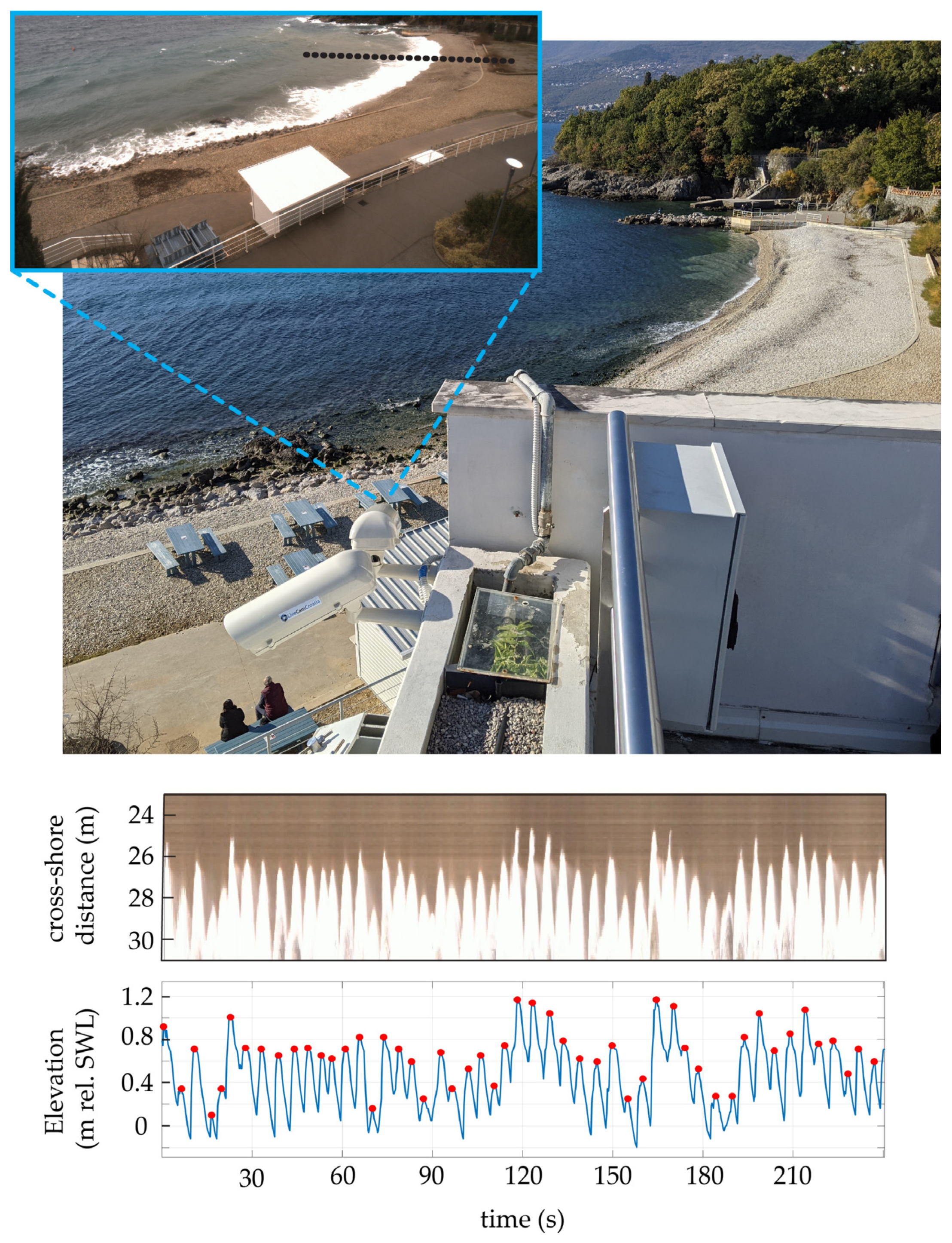
2.1. Study Site

Measurements of wave runup and the corresponding morphological response were carried out at the artificial pebble beach Ploče, located in the northwestern part of the city of Rijeka, Croatia, in the Kvarner Bay (Figure 1a–c). In 2011, two groynes were constructed on the east and west sides of the western beach cell (green zone in Figure 1c) to extend the beach area (Figure 1c). Currently, the total length of the beach is 320 m and is divided into two cells of approximately equal length by a 30 m long central groyne. The western beach cell (green zone in Figure 1c) is the focus of this study. Grains on the beach surface include sediment sizes (D₅₀) between 16–32 mm and can be classified as coarse gravel or pebbles. Rocks larger than D₅₀ > 0.2 m are located on the east side of the western cell of the beach. They are part of the central groyne, which increases the stability of the beach and prevents the transport of material from one beach cell to another.

In this study we used bathymetric measurements performed by the Geodetic Institute Rijeka (GZR) and the Faculty of Civil Engineering in Rijeka (GradRi) using a UAV and the photogrammetry method previously published in [57]. The topographic beach surveys were conducted nine times between 1 October 2020 and 26 February 2021 (UAV11 to UAV19 in Figure 2 and in

Table A1. Table of relevant UAV flight missions for beach surface measurements, from which beach profiles are extracted; this is an extract from the paper of Tadić, et al. [57].

Survey Label	Date	Number of Images	Flying Altitude (m)	Ground Res. (mm/pix)	Coverage Area (km²)	Reprojection Error (pix)
UAV_11	1.10.2020	535	28.1	7.53	0.0177	0.772
UAV_12	6.10.2020.	492	28.6	7.18	0.0199	0.826
UAV_13	13.10.2020.	538	28.5	7.12	0.0181	0.79
UAV_14	2.11.2020.	208	103	19.5	0.0802	0.733
UAV_15	24.11.2020.	278	20.5	5.08	0.00797	0.515
UAV_16	10.12.2020.	600	24.3	6.05	0.0172	0.315
UAV_17	14.12.2020.	560	26.7	6.62	0.0162	0.318
UAV_18	14.1.2021.	269	100	19.1	0.06	0.724
UAV_19	26.2.2021.	290	101	19.6	0.06	0.791

in Appendix A), mainly after storm wave events. A detailed point cloud of the entire beach surface was created for each UAV flight, while specific profiles (profiles 1–3 in Figure 1d and Figure 2) can be easily extracted afterwards. GZR used a Matrice 200 unmanned aerial vehicle (UAV) with a Sony ILCE-7M2 camera and GradRi used a DJI Phantom 4 Pro UAV for image acquisition. This technique showed good accuracy and efficiency for computing and mapping the spatial distribution and elevations [57]. It was demonstrated that the UAV mapping technique is accurate to about 0.7 pixels, or 4.2 cm in most cases. The reader is referred to [57] for the technique and detailed settings description of the UAV surveys.

Three representative profiles (profiles 1, 2 and 3 in Figure 1d and Figure 2) were selected for the assessment of wave runup on Ploče beach. They are located at the western side, at the midline and at the eastern side of the observed beach area of the western beach cell (Figure 1d). No profile was selected from the beach section, east of the profile 3, containing large rocks supported by a vertical concrete wall near the groyne. Beach slope is calculated and updated from topographic cross sections obtained from UAV survey. This time-varying beach slope is determined using a section of the beach profile from the still water level plus the significant wave height (SWL+H_s), down to the still water level minus twice the significant wave height (SWL-2H_s), a method previously introduced by [17,22,58]. The average slope of profile 1 at the westernmost part of the beach is slightly steeper (tanβ = 0.18) (Figure 2a) than that of profiles 2 and 3 (tanβ = 0.14) (Figure 2b,c).

The beach profiles 1 and 2 are primarily exposed to strong wind-driven waves from SSE, while the profile 3 is partially sheltered from the prevailing S and SSE wave by the groyne (environmental wave conditions and the associated wave climate are discussed in more detail in Section 2.3). Cases where the beach storm response could be determined as overtopping or overwashing are not considered in this work, only pure swash cases. This was based on the work by [59,60], who defined the regimes of overtopping and overwashing as situations where the freeboard is negative or the wave runup exceeds the height of the gravel barrier, while swash is defined with a positive freeboard.

2.2. Data Collection

Wave runup was measured with a video camera during the winter months and was derived from video images (Figure 1c and Figure 3). A coastal video monitoring system was installed in early October 2019 to monitor beach dynamics and behavior during storm events, as significant wave events in the eastern Adriatic occur mainly in winter. An Argus-type video monitoring system consisting of two cameras was installed on the roof of the indoor pool (Figure 1c and Figure 3). The camera model is the Blackfly S GigE camera (BFS-PGE-122S6C-C) with a resolution of 4096 × 3000 pixels, mounted 13.75 m above mean sea level (MSL) and capturing high-resolution video images at a frequency of 4 Hz.

Intrinsic and extrinsic calibration was performed for the cameras. First, intrinsic calibration is performed before the cameras are deployed according to the Camera Calibration Toolbox developed at Caltech [61]. Then, extrinsic calibration is performed following the CIRN Quantitative Coastal Imaging Toolbox [62]. In this toolbox, the raw images captured by the video system from the oblique view are converted into a georectified image from the bird’s eye view. This georectification process represents a geometric transformation of the raw image pixels into real coordinates. In this new view, features of the image, such as the position of cross sections, can be determined. The process of georectifying images required accurate three-dimensional (x,y,z) coordinates of the video monitoring system and several ground control points (GCPs). The GCPs were fixed and surveyed by the Geodetic Institute in Rijeka. They are located at static parts of the beach, namely the promenade and groynes. All points were measured in the Croatian Terrestrial Reference System HTRS96 (EPSG: 3765) in the horizontal plane and HRVS71 in the vertical direction.

Pixel stacks were sampled at 4 Hz for 12-min periods. The method developed by [63] was used to reduce the tidal shift during stack acquisition and maximize the size of the data set [17]. Using the CIRN Quantitative Coastal Imaging Toolbox, the leading edge of the runup maxima between water and beach was automatically digitized using intensity thresholds. If necessary, manual corrections were made to avoid blurring due to moving objects (e.g., birds, people) and to correct for false detections due to water lens debris on the beach during backwash [64]. The digitized waterline was converted from the cross-shore distance (Figure 3) with reference to the beach profile (Figure 2) to determine the water elevation along the pixel line [17]. Camera elevation and location affect the cross-shore resolution of the extracted pixel stack [63,65], nevertheless the horizontal cross-shore resolution was 0.2–0.45 m, which is consistent with previous studies [17]. Following Stockdon, et al. [4], wave runup was expressed as the 2% exceedance value, R_2%, derived from the cumulative density function of the discrete maximum wave runup heights (red dots in Figure 3). The wave runup was measured in different environmental conditions. The wave runup used for further analysis is the runup level, which does not exceed the gravel barrier crest. Taking these conditions into account, 152 wave runup measurements met the criteria and were selected for further analysis.

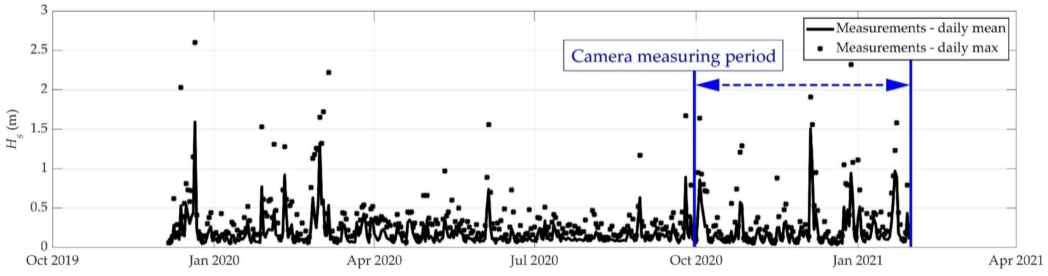
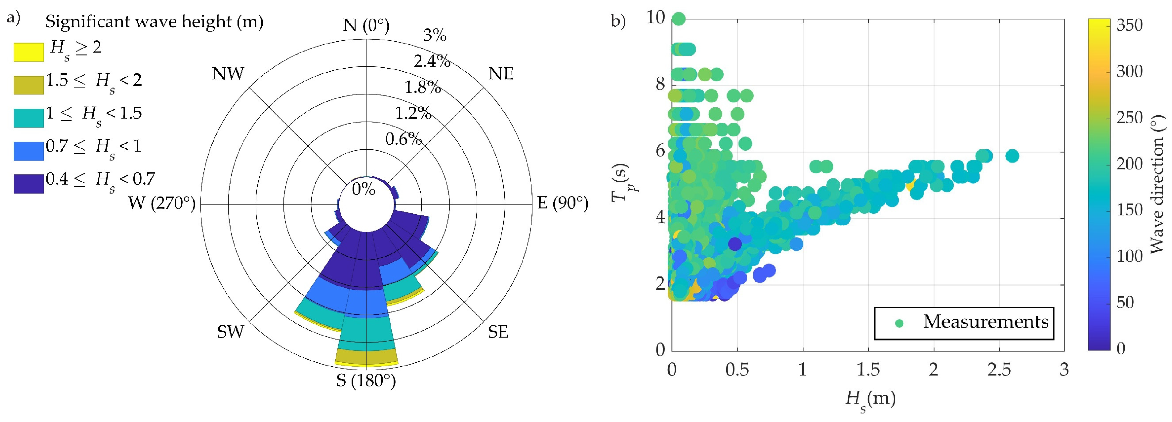
2.3. Evironmental Conditions

Wave parameters were obtained from wave buoy measurements. A wave buoy (DATAWELL DWR MKIII) deployed by the Hydrographic Institute of the Republic of Croatia, in cooperation with the Rijeka Port Authority at 57.5 m depth and measurements covered the camera observation period (Figure 1b).The wave buoy has a diameter of 0.7 m and its location off the coast of Rijeka was at the following geographic coordinates (WGS 84 system): Lat = 45°19′37.80″ N; Lon = 14°23′38.88″ E. The measurement data are stored in the buoy’s internal data logger with a capacity of 2 GB, but the data are also transmitted to the RX-C receiver on shore via the HF antenna connection on the buoy.

From the measurements taken for just over the year, it can be seen that calm conditions with daily significant wave heights up to 0.4 m are dominant (Figure 4). This is due to mild winds, which prevail here throughout the year. Periods of mild winds are intermitted with occasional storms with wind speeds exceeding 30 m/s, rarely lasting more than one day [57]. During these storm events, the maximum hourly significant wave height can reach up to 2.6 m (e.g., in December 2019), with daily average significant wave heights of more than 1.4 m. The most powerful winds in Kvarner Bay are the northeasterly, Bura, and the southeasterly, Jugo. However, the latter has larger fetch in the Kvarner Bay and accordingly higher wave heights and wave periods.

The wave rose in Figure 5 summarizes the hourly significant wave heights and directions recorded by the wave buoy. Figure 5 shows that the rare stormy wave events reach Ploče beach mainly from south and south-southeast directions. During the storms, the wave height increases more than the wave period, which leads to a steepening of the wave field. The wave steepness for these short wavelength waves is relatively steep compared to the open ocean waves, approximately H_s/L₀ = 0.04–0.05 during storm events.

Hourly tidal data are obtained from the nearby tidal gauge station, Bakar, at the northern tip of Bakar Bay (45°18.3′ N, 14°32.4′ E). The tides in the Adriatic Sea have mean tidal amplitudes well below 2 m and at the Bakar station, the mean daily tidal oscillations are 30 cm [66]. In this region, the relative tidal range (RTR = MSR/H_b, where MSR is the mean spring tidal range and H_b is the breaking wave height) is less than 1 and therefore is not dominated by the tides [67,68].

Therefore, the section of the beach profile exposed to wave swash changes only slightly during the tidal cycle, consequently the beach slope varies slightly. However, extremely high water levels (also called Acqua Alta) occasionally occur in this region when tides, storm surges, seiches, and other low-frequency sea level fluctuations overlap [69], but these were not recorded during this study.

2.4. Wave Runup Models and Error Metrics

Estimates from five wave runup equations proposed by [4,17,43,64] were compared with field measurements. The equations and the extent of the parameter space can be found in Appendix B (

Table A2. Table of relevant and well-known empirical wave runup equations tested on beach Ploče; associated range of conditions, beach, and measurement type are shown for each derived equation.

Reference	Equation	Range of Conditions	Measurement and Beach Type
Stockdon, et al. [4]	$R_2=1.1\left[\overline{\eta }+\frac{\sqrt{S_{ig}{}^2+S_{inc}{}^2}}{2}\right]$	$0.07<{\xi }_0<3.55$	Field measurements—sandy beach
	$\overline{\eta }=0.35\tan ({\beta }_S){\left(H_0{L}_0\right)}^{0.5}$	$0.0008<H_0/L_0<0.03$
	$S_{ig}=0.06{\left(H_0{L}_0\right)}^{0.5}$	$0.01<\tan ({\beta }_S)<0.16$
	$S_{inc}=0.75{\left(H_0{L}_0\right)}^{0.5}$
Poate, et al. [17]	$(\mathrm{a})R_2=0.49\tan {({\beta }_S)}^{0.5}{T}_Z{H}_0$	$2m<H_0<7.02m$	Field measurements—gravel beach
	$(\mathrm{b})R_2=0.33\tan {({\beta }_S)}^{0.5}{T}_p{H}_0$	$5.11s<T_p<19.55s$
Didier, et al. [64]	$R_2=0.117{\left(H_0{L}_0\right)}^{0.5}$	$0.3<{\xi }_0<2.5$	Field measurements—sandy, mixed and gravel beach
		$0.00023<D_{50}<0.16$
Holman and Sallenger [43]	$\frac{R_2}{H_0}=0.2+0.83{\xi }_0$	$0.07<{\xi }_0<3.25$	Field measurements—sandy beach

). These equations are hereafter referred to as P16a (Figure 7a), P16b (Poate, et al. [17], Figure 7b), D20 (Didier, et al. [64], Figure 7c), H85 (Holman and Sallenger [43], Figure 7d), and S06 (Stockdon, et al. [4], Figure 7e). Three of these equations (P16a, P16b and D20) are derived for gravel beaches, while S06 and H85 are derived for sandy beaches. These, and in particular S06, are considered here as these are included in many coastal engineering applications.

Morphological characteristics of the beach and their influence on the relative wave runup (a ratio of the wave runup and the significant wave height), are included in the wave runup equations in terms of the Iribarren number or the surf similarity parameter. The Iribarren number is a well-known dimensionless parameter used to combine the morphodynamic characteristics of the beach and surf zone with offshore wave parameters, and is commonly used in wave runup equations [4,10,29,32,43,47,70,71]. The Iribarren number is defined as follows:

$${\xi }_0=\frac{\tan (\beta )}{\sqrt{\frac{H_0}{L_0}}},$$

(1)

where tanβ is the beach slope, H₀ is the offshore deep water wave height and L₀ is deep water wavelength given by:

$$L_0=\frac{g{T}_p^2}{2\pi },$$

(2)

where T_p is the peak wave period, and g is the gravitational acceleration.

The variability of the relative wave runup depends on the reflectivity of the beach, which is determined by the Iribarren number (surf similarity parameter, ξ₀). In general, the relative wave runup increases as the reflectivity of the beach (the surf similarity parameter) increases.

It was also found [3] that including the significant wave height H_s and the peak wave period T_p are not sufficient for prediction of wave runup in certain cases but other features of the spectral shape need to be accounted for. In cases like bimodal seas, wave runup equations using only the peak wave period or the associated wavelength could be less accurate [17,72,73]. Therefore, some studies used the spectral period (estimated from different spectral moments) to account for the variability in the shape of the wave spectra. For example, P16a uses the mean wave period T_z as an equation input, in contrast to P16b, which uses the peak wave period T_p.

On the other hand, Polidoro, et al. [74] used the Goda peakedness parameter, Q_p, to increase the explanatory power of the equation for wave runup. The Goda peakedness value, Q_p, of the wave spectrum, referred to in Section 3.3 and Section 3.4, is defined as:

$$Q_p=\frac{2}{m_0^2}{\displaystyle \int f·S^2\left(f\right)}df$$

(3)

where S(f) is the one-dimensional frequency-energy density spectrum and f is the frequency, and m₀ = (H_s/4)².

The measured runup statistics are compared with prediction from the runup equations. The accuracy of the wave runup equations is examined using the Pearson correlation coefficient (R), the corrected scatter indicator HH proposed by [1], the normalized bias (NBIAS), and the normalized root mean square error (NRMSE), defined in Equations (2)–(5) respectively:

$$R=\frac{{\displaystyle \sum _{i=1}^N\left(\left(P_i-\overline{P}\right)\left(O_i-\overline{O}\right)\right)}}{{\left[\left({\displaystyle \sum _{i=1}^N{\left(P_i-\overline{P}\right)}^2}\right)\left({\displaystyle \sum _{i=1}^N{\left(O_i-\overline{O}\right)}^2}\right)\right]}^{1/2}}$$

(4)

$$HH=\sqrt{\frac{{\displaystyle \sum _{i=1}^N{\left(P_i-O_i\right)}^2}}{{\displaystyle \sum _{i=1}^N{P}_i{O}_i}}}$$

(5)

$$NBIAS=\frac{\overline{P}-\overline{O}}{\overline{O}}$$

(6)

$$NRMSE=\sqrt{\frac{{\displaystyle \sum _{i=1}^N{\left(P_i-O_i\right)}^2}}{{\displaystyle \sum _{i=1}^N{O}_i{}^2}}}$$

(7)

where P_i is the ith prediction of the evaluated model, O_i the ith observation captured by the camera system and N is the number of data points in the time series (or the number of usable footages from the camera system, in this study N = 152). The overbar indicates the mean values, as in $\overline{P}$ is the mean of all prediction values, and $\overline{O}$ is the mean of all observation values. P_i, O_i, $\overline{P}$ and $\overline{O}$ are case specific descriptions for model accuracy evaluation instead of a more general mathematical description of x_i, y_i, $\overline{x}$ and $\overline{y}$ in Equations (4)–(7). For both HH and NRMSE performance indicators, a larger value indicates a higher dispersion error, while a lower value indicates a lower dispersion error when comparing measured and modeled data. Both indicators are always non-negative and show perfect agreement between measured and modeled data at a value of 0.

3. Results

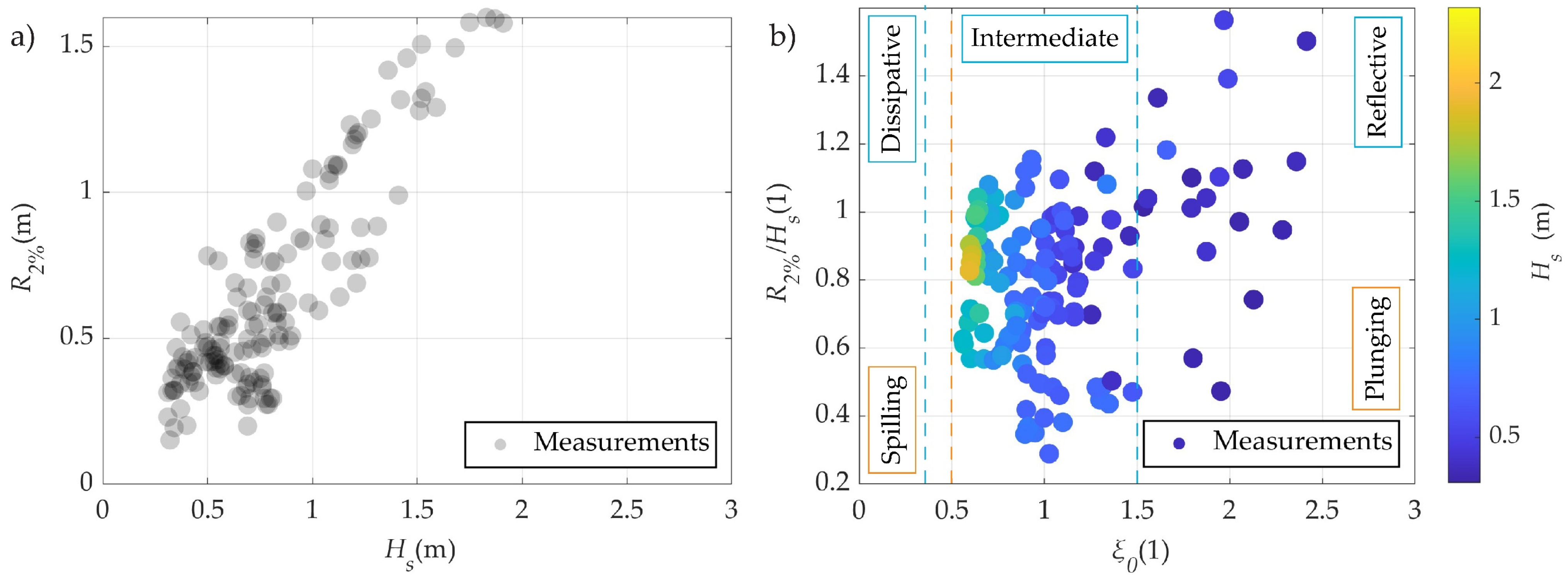
3.1. Description of Field Measurements for the Centerline Profile (Profile 2)

This section shows the wave runup obtained by processing the time-stack images (described in Section 2.2). Significant wave heights, H_s, up to H_s = 2.32 m, with an associated wave period of 5.8 s were recorded in the time period when both the video camera and the wave buoy operated. Wave events with highest significant wave heights resulted in overtopping of the gravel barrier and promenade behind the beach and were therefore excluded from further analysis of wave runup. After excluding events where the gravel barrier crest was overtopped, the maximum observed significant wave height was H_s = 1.85 m (Figure 6a), with an associated wave peak period of 5.5 s. The values of wave runup for all available video segments (N = 152) from early October 2020 to late January 2021 are shown in Figure 6. They increase with the increase in significant wave height offshore, indicating that the swash did not reach saturation during the observation period and for measurements included here (Figure 6a). However, wave runup values vary for the same offshore significant wave height.

Figure 6b shows relative wave runup (ratio of wave runup to significant wave height, R_2%/H_s) as function of the Irribaren number for different significant wave heights (different colors). The beach itself shows reflective behavior (ξ_o > 1.5) in milder wave conditions, while it shows intermediate behavior (ξ_o $\approx$ 0.65 for H_s > 1.5 m) in extreme wave conditions. However, the relative wave runup at extreme wave conditions shows a weak dependence on the surf similarity parameter, with all extreme wave conditions showing a similar Irribaran number of ξ_o $\approx$ 0.65. All observed wave breaker types belong to the group of “plunging breakers”, which were also observed on the camera video data (Figure 3). Variability in measured relative wave runup is even more pronounced than in measured wave runup for the same offshore significant wave height. The observed range of relative runup values range is from 0.2 to 1.6. Even for energetic wave conditions (H_s > 1.5 m), the variability of the relative wave runup is high, with values in the range of 0.6 < R_2%/H_s < 1.1 (almost twice the relative wave runup from minimum to maximum). These indicate that the values of the relative wave runup can differ significantly for the same significant wave height offshore.

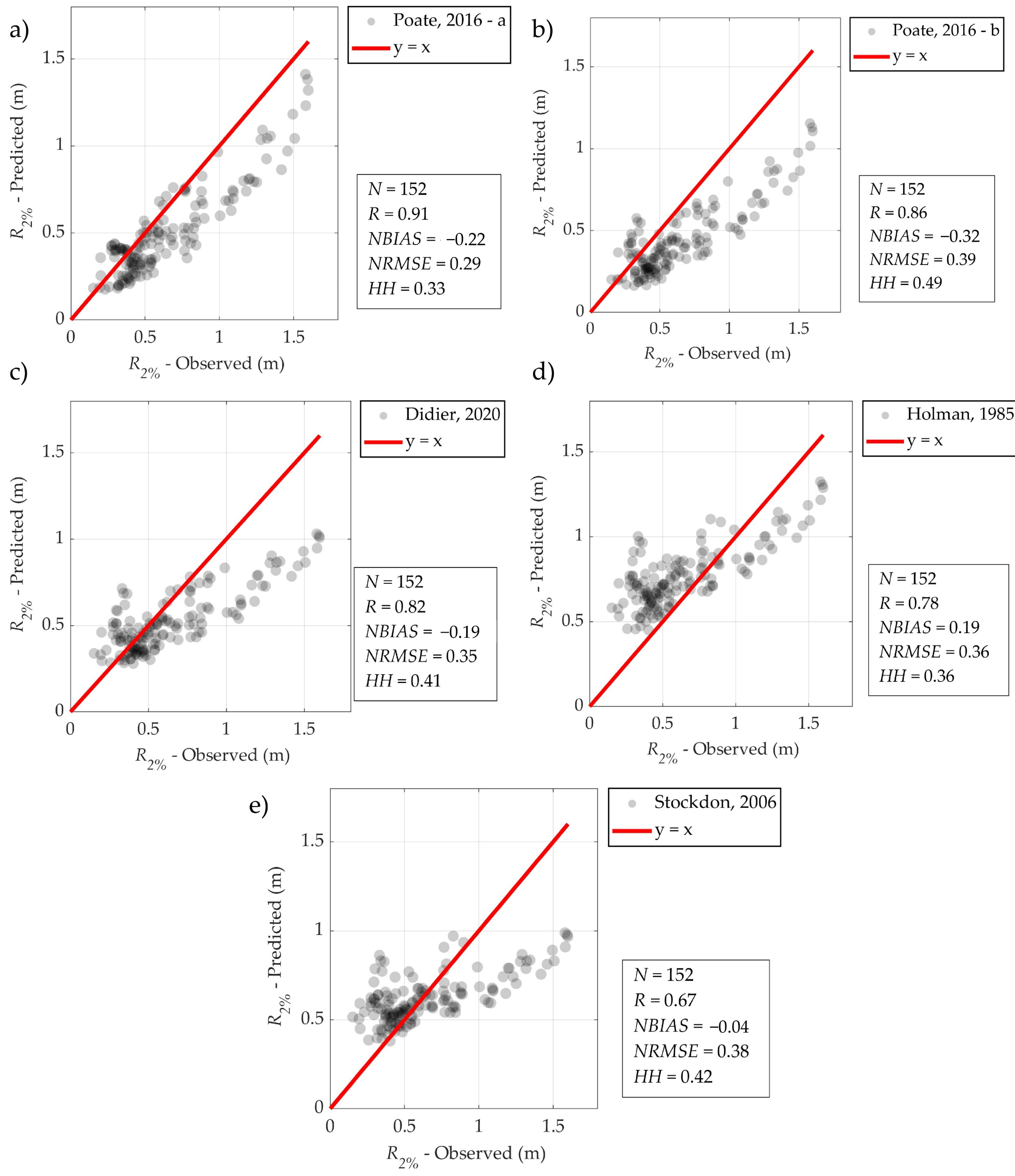
3.2. Comparison with Existing Wave Runup Equations for the Centerline Profile (Profile 2)

In this section, the capability of the existing equations for prediction of wave runup for a micro-tidal gravel beach in fetch-limited wave conditions is examined and compared. Figure 7a–e show the scatter plots between the predicted and observed R_2% for each tested empirical equation for wave runup. Predicted wave runup values using equations, P16a, P16b, D20, H85 and S06 (see Section 2.4 and Appendix B) are plotted versus measured (observed) values in Figure 7. The y = x line shows a perfect fit between the two, and the accuracy parameters are shown next to the scatter plots.

Equation P16a (Figure 7a), formulated specifically for straight pure gravel beaches in unlimited fetch conditions, showed the best accuracy in predicting observed wave runup (R = 0.91, NRMSE = 0.29 in Figure 7a). Using the peak wave period T_p in equation P16b, instead of the mean wave period T_z in P16a, reduced the accuracy of the equation (35% increase in NRMSE) (R = 0.87, NRMSE = 0.39 in Figure 7b). Both equation P16a and equation P16b for wave runup show significant underprediction over the entire range of observed wave runup values (NBIAS = −0.22 and NBIAS = −0.32 for P16a and P16b, respectively). The D20 wave runup equation derived for fetch-limited wave situations showed slightly lower accuracy than the P16a gravel equation (10% lower correlation and 21% higher NRMSE). The NBIAS also showed underprediction, although to a slightly lesser extent than the P16a equation. As expected, equations H85 and S06 for wave runup derived from measurements at open sandy beaches showed the lowest accuracy (R = 0.78 and 0.67 with NRMSE = 0.36 and 0.38 for equations H85 and S06, respectively).

All equations show higher accuracy for low wave runup situations (data are closer to the y = x line for the perfect fit in Figure 7a–e), but as wave runup (and thus offshore wave energy) increases, all equations tend to underestimate to some extent (up to 33% for S06).

Since P16a showed the best accuracy (both strong correlation and small NRMSE) in prediction of the measured wave runup, it has been chosen for further modifications to improve the wave runup predictions for conditions measured in this study, in Section 3.3.

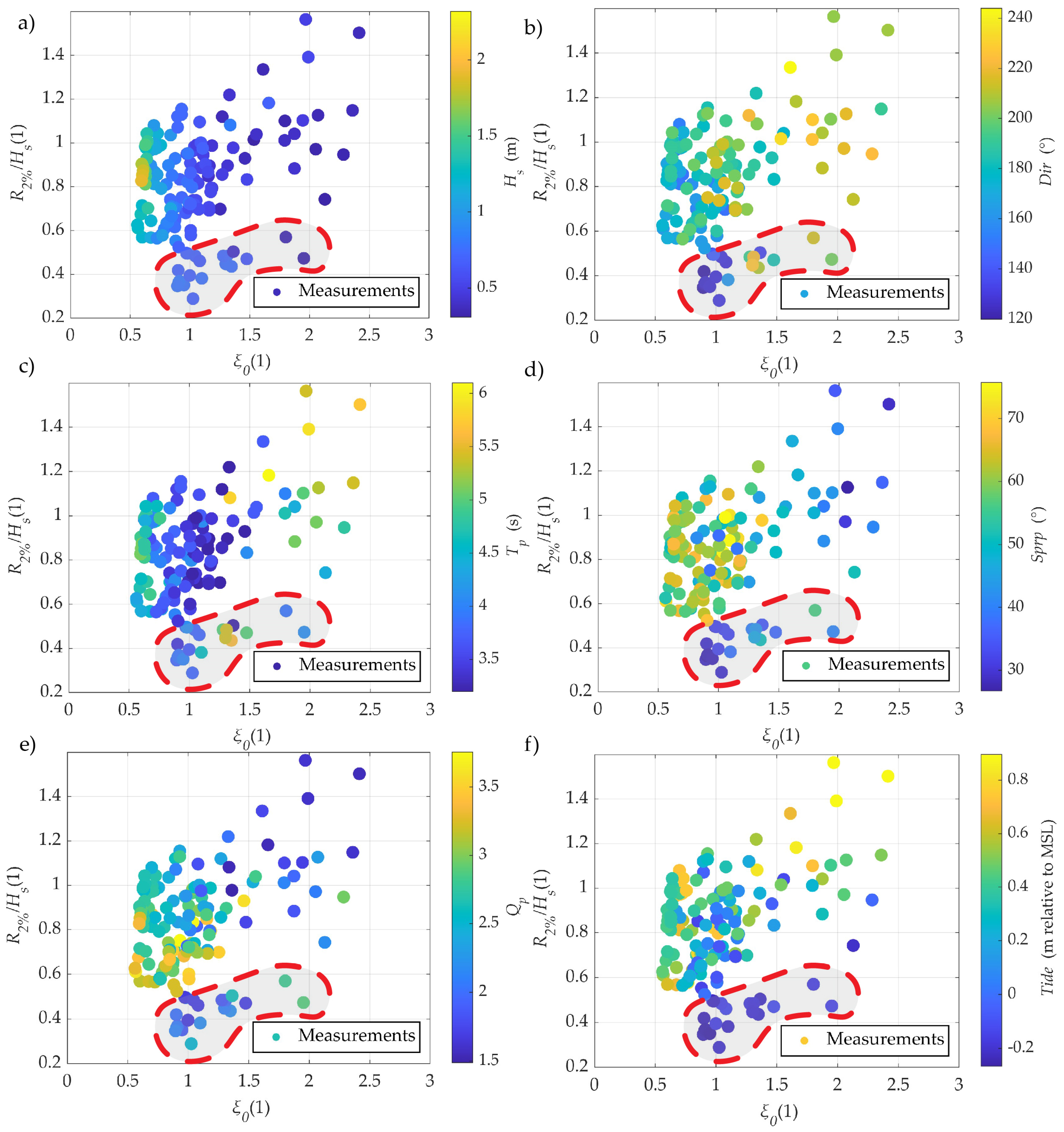
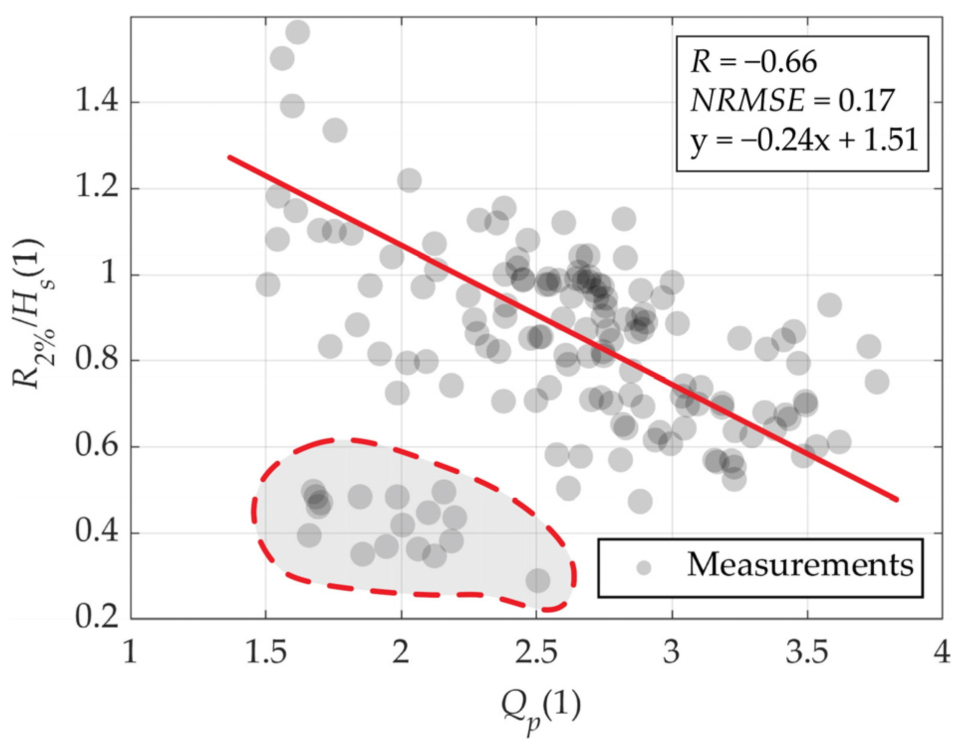
3.3. Influence of Offshore Wave Spectra Parameters on Wave Runup for the Centerline Profile (Profile 2)

Figure 8 shows the relationship between relative wave runup and the offshore surf similarity parameter (Irribaren number) as in Figure 6b but, here, each plot examines the effect of a different wave parameter and a tidal level. Wave parameters and tidal levels are divided into different classes (see color bars) and the data points are colored accordingly. These graphs show that some of these parameters can provide additional explanatory power for the variability of the measured wave runup.

There is a cluster of data points (grouped together and separated from the rest of data points) that reduced the correlation between the relative wave runup and the Irribaren number (this specific cluster is in the area enclosed by a red dashed line in Figure 8). The relative wave runup is below 0.6 for all data measured at very low tidal levels (at −0.2 m below MSL in Figure 8f), for offshore waves with low significant wave heights (H_s < 0.5 m, in Figure 8a), with small directional wave spread (only 30°–50°, in Figure 8d) and an oblique wave direction of 120°–140° (in Figure 8b). For these wave directions, the beach is sheltered to a considerable extent by the rock groyne east of the pocket beach (Figure 1c). The groyne sheltering effect in combination with the lower tides (and thus shallower water depth) resulted in earlier and stronger wave breaking and thus a reduction in relative wave runup. Wave runup for this cluster of points is also small as both the relative wave runup and the offshore significant wave height is small. This makes the rest of the data more relevant, for studies of the effects of waves on the shoreline from a coastal engineering perspective.

Next, a correlation between the wave runup and the Goda peakedness parameter from offshore wave spectra, Q_p is examined in Figure 9 as some grouping of data is detected in Figure 8e. When the cluster of wave events (within the area enclosed by a red dashed line in Figure 8) are not considered, a significant correlation between the relative wave runup and the Goda peakedness parameter is found. As the Goda peakedness parameter increases the relative wave runup tends to decrease. There is a significant correlation of R = −0.66 between Q_p and R_2%/H_s.

Since the Goda peakedness parameter (Q_p) has a significant correlation with relative wave runup (Figure 9), the empirical equation for wave runup P16a is modified by including the Q_p parameter into the equation. Poate’s empirical equation, specifically P16a, was chosen because it showed the best accuracy in predicting wave runup measured at Ploče Beach (Figure 7). The Goda peakedness parameter Q_p is incorporated into the P16a equation in the following way:

$$R_2=0.49\tan {({\beta }_S)}^{0.5}{T}_Z{H}_0·{\left(\frac{a}{Q_p}\right)}^b$$

(8)

where the part of the equation marked in blue is from the original P16a equation (βs is the foreshore slope, T_z is the mean wave period, H₀ is significant wave height), and Q_p is the newly included Goda peakedness parameter, while a and b are constants, which can be determined from measurements.

A genetic algorithm is used to search the parameter space to determine the constants a and b with the aim of finding the global minimum of the defined loss function [75,76]. The loss function for the genetic optimization algorithm is defined as the NRMSE according to Equation (7), between the measured wave runup (O in Equation (7)) and predicted values of the wave runup according to eq. 8 (P in Equation (7)). The population size is set to 200, with a run of 15,200 generations. The obtained values for coefficients a and b are 6.03 and 0.29, respectively. With the included values for the coefficients a and b, Equation (8) takes the following form:

$$R_2=0.82\tan {({\beta }_S)}^{0.5}{T}_Z{H}_0{Q}_p^{-0.29}$$

(9)

Figure 10 shows a strong increase in accuracy using the modified Equation (9) compared to the original P16a equation for wave runup. The dimensional constant on the right-hand side of Equation (9) contains a unit of s⁻¹, showing the empirical nature of the equation. The NRMSE decreased by 31% compared to the P16a equation and eliminated the NBIAS (R = 0.91, NRMSE = 0.20, NBIAS = 0).

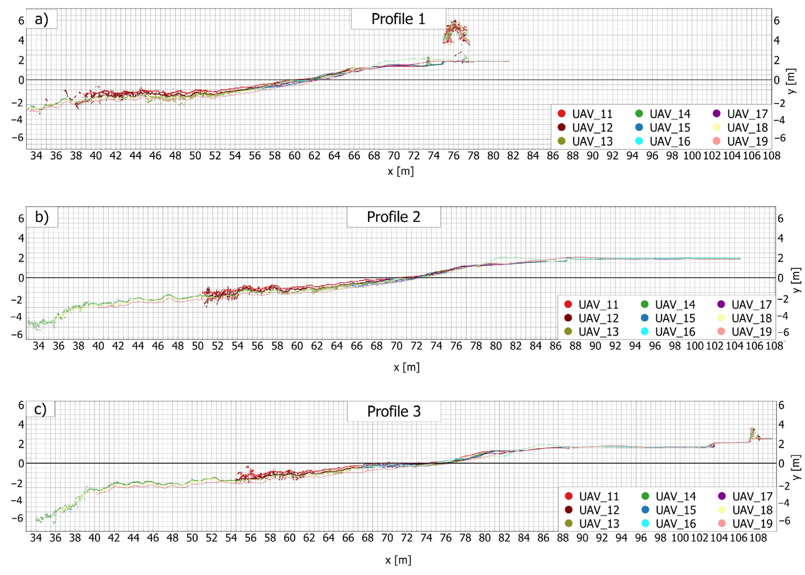
3.4. Alongshore Variability of Wave Runup

Figure 11 compares wave runup (R_2%) measured at the centerline profile (profile 2 in Figure 1d) with runup measured at the profiles to the west and east (profiles 1 and 3, respectively, in Figure 1d).

The scatter plots show that the wave runup measured at the centerline and the west profile is strongly correlated (Figure 11a) (R = 0.96 and NRMSE = 0.16). However, wave runup values on the west profile are 20% larger than those on the centerline profile. On the other hand, the relationship between the wave runup at centerline profile and the eastward profile is not as strong, but still significant (R = 0.87 and NRMSE = 0.37). In this case, the values of the wave runup for the east profile are 29% smaller than those on the centerline profile.

Two factors that potentially influence the observed difference, the alignment of the wave direction with the direction of the beach profiles and beach slope, are examined here.

By comparing, the direction of each profile 1, 2, and 3 (west, centerline and east, respectively) with the dominant wave direction S and SSE (the mean wave direction is 172° for wave events with significant wave heights, H_s > 1 m), it is evident that profile 1 (at 192°) is more aligned with the dominant wave direction than profile 2 (at 205°) and especially profile 3 (at 216°). Moreover, the groyne located to the east has a sheltering effect to the profile 3 for waves from the prevailing SE wave direction (Figure 1d). These differences can partly explain a weaker correlation between the wave runup measured on the profiles 2 and 3 and the larger scatter observed in Figure 11b.

Another factor is beach slope, which is included in Equation (9), P16a and P16b. A steeper beach profile leads to an increase in wave runup. With this in mind, we can observe that the western beach slope (profile 1) is steeper than both profiles 2 and 3 (tanβ = 0.18 for profile 1 and tanβ = 0.14 for profiles 2 and 3). Consequently, a steeper beach slope of profile 1 also contributed to an increase in wave runup.

Overall, with a stronger alignment to the prevailing wave direction and a steeper beach profile, larger wave runup values are expected.

4. Discussion

4.1. Wave Runup

The wave runup shows a strong lineasr relationship with the significant wave height (Figure 6a). There is no indication of saturation of the wave runup. One of the reasons is that the highest wave runup events leading to wave overtopping were not considered here. Another possible reason is that beaches which display significant wave reflectivity, show no saturation of wave runup according to Guza, et al. [77], Guza and Bowen [78]. Wave runup increases with incident significant wave height, just as at Ploče beach, which indicates relatively low energy dissipation at least for conditions considered here. The same behavior was also observed by Guza and Thornton [29] in southern California.

4.2. Application of Existing Wave Runup Equations

A number of different wave runup equations, derived on the basis of laboratory and field measurements, exist and are used by the research community and practitioners. However, all of them have limited applicability in terms of the range of input parameters and are most appropriate for the environmental conditions for which they were developed. In this study, a selection of the most appropriate and well-known wave runup equations [4,17,43,64] (see Appendix B) were used for the calculation of wave runup on Ploče beach, an artificial fetch-limited gravel pocket beach.

Predictions of wave runup using eq. P16a were the most accurate. This is not so surprising considering that the equation was developed for gravel beaches. However, the equation was applied for fetch-limited gravel beaches, conditions not considered before. In addition, both equation P16a and equation P16b were developed from data with high significant wave heights (2 m < H_s < 7.02 m) and associated peak wave periods (5.11 s < T_p < 19.55 s) whereas waves measured offshore of Ploče beach are outside the range of applicability of equations P16a and P16b. The equations are derived for steeper beach slopes (tanβ = 0.07–0.4), which were similar for the beach Ploče. It is interesting to note that eq. P16b, which uses the peak wave period, has a lower accuracy in predicting the wave runup. This is in agreement with the finding from the original work of Poate, et al. [17]. In the original work, the authors concluded that the peak wave period, T_p, cannot convey enough information for a complex wave spectrum, such as a bimodal spectrum. Unfortunately, no spectrum information was made available with the wave data to examine how spectrum shape affects wave runup. Instead, the Goda peakedness parameter, Q_p, was used, and it was found that there is a correlation between wave runup and this parameter. Inclusion of the Goda peakedness parameter into equation P16a improved its accuracy (Section 3.3), suggesting that additional spectral information could be included in the wave runup equation.

Predictions of wave runup by using the D20 equation were slightly less accurate than those obtained using P16a. This is despite the fact that this equation was derived from measurements in fetch-limited environment and that the other parameters measured at Ploče Beach are within the range of measured parameters used for derivation of the D20 equation (0.3 < ξ_o < 2.5 and 0.00023 m < D₅₀ < 0.16 m). The lower accuracy was likely due to other factors, such as the exclusion of beachface slope or swash zone slope from the wave runup equation, as described in [35]. The swash zone is often very narrow at fetch-limited beaches [79], while gravel sediment, such as on Ploče beach, promotes further beach steepening and thus swash zone narrowing. As expected, predictions of wave runup using equations H85 and S06 derived for sandy beaches, as expected, were the least accurate. Eq. S06, which is a widely used equation for wave runup predictions, underpredicted measured runup by over 30% for the most energetic wave events. The underprediction by S06 has already been noted in the literature in some other cases where the surf zone is narrow or absent [17,80], as equation S06 was developed for sandy conditions with broad surf zones.

4.3. Derivation of the New Runup Equation for Fetch-Limited Gravel Pocket Beach Cases

Equation P16a, which yielded the most accurate wave runup on Ploče beach (R = 0.91, NRMSE = 0.29 m, HH = 0.33), was selected for further modification and refinement, with an aim of improving the fit between precited and measured wave runup at Ploče Beach. While the eq. P16a predictions were the most accurate, they still showed substantial underprediction of 22% (NBIAS = −0.22), with some points underpredicting up to 50% (observed runup of R_2% = 1.5 m and predicted runup of R_2% = 1.0 m by eq. P16a in Figure 7a). While predictions from the P16a equation showed a good fit with the original data measured in the UK from which it was derived, the dimensional constant on the right-hand side of the equation (Equation (10)) implies that the equation is appropriate only to use in environments with similar wave and beach conditions. The wave conditions on Ploče beach are outside the range of applicability of the equation P16a (2 m < H_s < 7.02 m) and as it is pointed out the equation needs to be reassessed if used outside of its initial application range [17].

Additional parameters that could potentially improve the wave runup predictions were also examined. As discussed in [3], different wave spectra could have the same significant wave height H_s and peak wave period T_p, but other features of the spectral shape could be left unaccounted for in the empirical equation for wave runup. Consequently, wave runup equations using only the peak wave period or the associated wavelength could be less accurate [17,72,73]. Therefore, some studies used the spectral period (estimated from different spectral moments) to account for the variability in the shape of the wave spectra, while Polidoro, et al. [74] used the Goda peakedness parameter, Q_p.

The wave runup data measured at the Ploče beach showed that the Goda peakedness parameter, Q_p, is inversely proportionate to the wave runup. In other words, an increase in Q_p decreased the wave runup, R_2%. The same was found in the work of Polidoro, et al. [74]. The Q_p parameter was included in the derived equation for wave runup and applied on mixed sand and gravel beaches with extreme bimodal climate. Equally, Polidoro, et al. [74] also observed an inverse effect of the Q_p parameter on the wave runup.

The modified eq. P16a, which included the Goda peakedness parameter, Q_p, and the associated coefficients removed the bias completely from the prediction (from a underprediction of 22% to 0% bias) and reduced the NRMSE by 31%. Site-specific tuning for improving local runup predictions was suggested in [81] as a viable procedure for improving accuracy, but it highlights the importance of environmental conditions at each new site similar to those at the original site for which the equation was derived. Even though the complexity of the new Equation (9) is somewhat increased due to the inclusion of Qp, it is still significantly less complex when compared to the well-known S06 equation (see Table A2). Clearly, the newly developed Equation (9) should be further tested, and additional corrections explored when used under similar wave conditions and on similar beaches. Unfortunately, measurements of wave runup in similar conditions on pocket beaches are extremely rare due to the inherent variability of wave runup along the shoreline, and research rarely addresses this complexity, as noted by [18].

4.4. Effects of Tides and Groundwater Dynamics

Ploče beach is a microtidal beach [23,56,82,83], with an RTR below 1 [64] and hence the influence of the variation in tidal levels on wave runup was not examined. Nevertheless, a cluster of relatively smaller wave runup heights compared to the rest of wave runup was measured at extremely low tide and for oblique wave directions. The remaining of the scatter between predictions using Equation (9) and measurements can be due to a number of different factors, e.g., non-linear interaction between wave runup and beach slope, parameters not included in equations and possibly due to errors in the measured data due to measurement techniques. Nevertheless, the method used is consistent with previously established studies of wave runup observation [4,27,31,84]. Moreover, the swash permeability and groundwater dynamics could add an additional layer of uncertainty [85,86]. Kobayashi, et al. [87] showed that higher swash permeability lowers the expected wave runup on the shoreline. The region where Ploče beach is located is also known for strong groundwater flows from the inland to the sea. These flows are also known to occur at Ploče beach during heavy rains, when emerging flows erode the beach surface and push the gravel down the beach slope and offshore.

4.5. Alongshore Wave Runup Variability

Previous studies rarely consider the alongshore variability of wave runup and only observed wave runup at one beach profile at a time. Gomes da Silva, et al. [3] noted this limitation and called for studies that examine and report the variability of wave runup that represents the real wave condition of a beach. This assumption of low variability in wave runup could be justified for long straight beaches with minimal alongshore variability in beach orientation and morphology. However, the embayed shape of the Ploče beach surrounded by artificial headland-like groynes, results in alongshore variability of the significant wave height and resulting wave runup. On the beach of Ploče we observed an increase in wave runup with increasing alignment of the beach to the wave direction, in combination with a steeper slope, which both contributed to the increase in wave runup on the western profile. The increase in wave runup is 71% from the east to the west profile. This is still significantly lower than the variability observed by [44] on a beach influenced by sand waves with a 3-fold variation in wave runup.

5. Conclusions

This study presents, to our knowledge, first measurements of wave runup on a microtidal artificial pocket beach (or small embayed beach) of gravel sediment (D₅₀ = 3 mm) under fetch-limited wave conditions—Ploče beach in Croatia, which is typical for the eastern Adriatic coast. Wave runup at three profiles along the beach was measured using an Argus-type video camera during a 4-month field observation campaign (described in Section 2.1), covering a range of wave conditions. Time stack data were processed to extract wave runup events, which were then statistically processed (described in Section 2.2). The measured wave runup was compared with predictions from five well known and widely used empirical wave runup equations. The best match between measured and predicted runup was obtained for the Poate, et al. [17] equation P16a equation, which was developed for prediction of wave runup on pure gravel beaches.

A modified equation, based on the P16a equation was developed by adding the Goda peakedness factor, Q_p, to improve its predictions. The coefficient values were obtained by using a genetic algorithm. The statical metrics of the modified equation obtained in this paper are as follows: R = 0.91, NBIAS = 0, NRMSE = 0.2, HH = 0.2. The newly developed Equation (9) completely eliminated the bias (NBIAS = 0) and reduced the NRMSE by 31% in comparison to the unaltered P16a equation.

There was significant alongshore variability in measured wave runup, which increased by 71% from the east to the west profile. Specifically, 29% lower wave runup was measured at the eastern profile than on the centerline profile, while wave runup measured at the western profile showed 19% higher values than on the centerline profile. This observed alongshore variability is due to different orientation of beach profiles and resulting difference in alignments to the prevailing wave direction. In addition, beach profile slopes increased from east to west, from tanβ = 0.14 at profile 2 and 3 to tanβ = 0.18 at profile 1.

Further measurements of wave runup on pocket gravel beaches in fetch-limited conditions are needed to validate the newly developed equation for prediction of wave runup. As with all empirical equations, the user needs to take into account the environmental conditions in which this equation is derived.

References

1. Longuet-Higgins, M.S.; Stewart, R.W. Radiation stresses in water waves; a physical discussion, with applications. Deep Sea Res. Oceanogr. 1964, 11, 529–562. [Google Scholar] [CrossRef]
2. Miche, M. Le Povoir Réfléchissant des Ouvrages Maritimes Exposés à L’action de la Houle. Ann. Ponts Chaussées 1951, 121, 285–319. [Google Scholar]
3. Gomes da Silva, P.; Coco, G.; Garnier, R.; Klein, A.H.F. On the prediction of runup, setup and swash on beaches. Earth-Sci. Rev. 2020, 204, 103148. [Google Scholar] [CrossRef]
4. Stockdon, H.F.; Holman, R.A.; Howd, P.A.; Sallenger, A.H. Empirical parameterization of setup, swash, and runup. Coast. Eng. 2006, 53, 573–588. [Google Scholar] [CrossRef]
5. Ruiz de Alegria-Arzaburu, A.; Masselink, G. Storm response and beach rotation on a gravel beach, Slapton Sands, UK. Mar. Geol. 2010, 278, 77–99. [Google Scholar] [CrossRef]
6. Coco, G.; Senechal, N.; Rejas, A.; Bryan, K.R.; Capo, S.; Parisot, J.P.; Brown, J.A.; MacMahan, J.H.M. Beach response to a sequence of extreme storms. Geomorphology 2014, 204, 493–501. [Google Scholar] [CrossRef] [Green Version]
7. Tomás, A.; Méndez, F.J.; Medina, R.; Jaime, F.F.; Higuera, P.; Lara, J.L.; Ortiz, M.D.; Álvarez de Eulate, M.F. A methodology to estimate wave-induced coastal flooding hazard maps in Spain. J. Flood Risk Manag. 2016, 9, 289–305. [Google Scholar] [CrossRef]
8. Butt, T.; Russell, P. Hydrodynamics and cross-shore sediment transport in the swash-zone of natural beaches. J. Coast. Res. 2000, 16, 255–268. [Google Scholar]
9. Elfrink, B.; Baldock, T. Hydrodynamics and sediment transport in the swash zone: A review and perspectives. Coast. Eng. 2002, 45, 149–167. [Google Scholar] [CrossRef]
10. Van der Meer, J.W.; Stam, C.J.M. Wave runup on smooth and rocky slopes of coastal structures. J. Waterw. Port Coast. Ocean Eng. 1992, 118, 534–550. [Google Scholar] [CrossRef]
11. Madsen, P.A.; Sørensen, O.R.; Schäffer, H.A. Surf zone dynamics simulated by a Boussinesq type model. Part II: Surf beat and swash oscillations for wave groups and irregular waves. Coast. Eng. 1997, 32, 289–319. [Google Scholar] [CrossRef]
12. Lange, A.M.Z.; Fiedler, J.W.; Becker, J.M.; Merrifield, M.A.; Guza, R.T. Estimating runup with limited bathymetry. Coast. Eng. 2021, 172, 104055. [Google Scholar] [CrossRef]
13. Gao, J.L.; Ma, X.Z.; Dong, G.H.; Chen, H.Z.; Liu, Q.; Zang, J. Investigation on the effects of Bragg reflection on harbor oscillations. Coast. Eng. 2021, 170, 103977. [Google Scholar] [CrossRef]
14. Liang, D.; Gotoh, H.; Khayyer, A. Boussinesq modelling of solitary wave and N-wave runup on coast. Appl. Ocean Res. 2013, 42, 144–154. [Google Scholar] [CrossRef]
15. Henderson, C.S.; Fiedler, J.W.; Merrifield, M.A.; Guza, R.T.; Young, A.P. Phase resolving runup and overtopping field validation of SWASH. Coast. Eng. 2022, 175, 104128. [Google Scholar] [CrossRef]
16. Tsung, W.S.; Hsiao, S.C.; Lin, T.C. Numerical simulation of solitary wave run-up and overtopping using Boussinesq-type model. J. Hydrodyn. Ser. B 2012, 24, 899–913. [Google Scholar] [CrossRef]
17. Poate, T.G.; McCall, R.T.; Masselink, G. A new parameterisation for runup on gravel beaches. Coast. Eng. 2016, 117, 176–190. [Google Scholar] [CrossRef] [Green Version]
18. Lashley, C.; Bertin, X.; Roelvink, D. Field measurements and numerical modelling of wave run-up and overwash in the pertuis Breton embayment, France. In Proceedings of the 7th International Conference on the Application of Physical Modelling in Coastal and Port Engineering and Science (Coastlab18), Santander, Spain, 22–26 May 2018; pp. 1–10. [Google Scholar]
19. Nicolae Lerma, A.; Pedreros, R.; Robinet, A.; Senechal, N. Simulating wave setup and runup during storm conditions on a complex barred beach. Coast. Eng. 2017, 123, 29–41. [Google Scholar] [CrossRef]
20. Mase, H. Random wave runup height on gentle slope. J. Waterw. Port Coast. Ocean Eng. 1989, 115, 649–661. [Google Scholar] [CrossRef]
21. Melby, J.A.; Nadal-Caraballo, N.C.; Kobayashi, N. Wave RunUp prediction for flood mapping. Coast. Eng. 2012, 33. [Google Scholar] [CrossRef] [Green Version]
22. Roberts, T.M.; Wang, P.; Kraus, N.C. Limits of wave runup and corresponding beach-profile change from large-scale laboratory data. J. Coast. Res. 2010, 261, 184–198. [Google Scholar] [CrossRef]
23. Atkinson, A.L.; Power, H.E.; Moura, T.; Hammond, T.; Callaghan, D.P.; Baldock, T.E. Assessment of runup predictions by empirical models on non-truncated beaches on the south-east Australian coast. Coast. Eng. 2017, 119, 15–31. [Google Scholar] [CrossRef] [Green Version]
24. Gomes da Silva, P.; Medina, R.; Gonzalez, M.; Garnier, R. Infragravity swash parameterization on beaches: The role of the profile shape and the morphodynamic beach state. Coast. Eng. 2018, 136, 41–55. [Google Scholar] [CrossRef]
25. Holman, R. Extreme value statistics for wave run-up on a natural beach. Coast. Eng. 1986, 9, 527–544. [Google Scholar] [CrossRef]
26. Power, H.E.; Gharabaghi, B.; Bonakdari, H.; Robertson, B.; Atkinson, A.L.; Baldock, T.E. Prediction of wave runup on beaches using Gene-Expression Programming and empirical relationships. Coast. Eng. 2019, 144, 47–61. [Google Scholar] [CrossRef]
27. Ruggiero, P.; Komar, P.D.; McDougal, W.G.; Marra, J.J.; Reggie, A. Wave runup, extreme water levels and the erosion of properties backing beaches. J. Coast. Res. 2001, 17, 407–419. [Google Scholar]
28. Vousdoukas, M.I.; Wziatek, D.; Almeida, L.P. Coastal vulnerability assessment based on video wave run-up observations at a mesotidal, steep-sloped beach. Ocean Dyn. 2012, 62, 123–137. [Google Scholar] [CrossRef]
29. Guza, R.T.; Thornton, E.B. Swash oscillations on a natural beach. J. Geophys. Res. 1982, 87, 483–491. [Google Scholar] [CrossRef]
30. Nielsen, P.; Hanslow, D.J. Wave runup distributions on natural beaches. J. Coast. Res. 1991, 7, 1139–1152. [Google Scholar]
31. Ruessink, B.G.; Kleinhans, M.G.; Van Den Beukel, P.G.L. Observations of swash under highly dissipative conditions. J. Geophys. Res. 1998, 103, 3111–3118. [Google Scholar] [CrossRef]
32. Gallien, T.W.; Sanders, B.F.; Flick, R.E. Urban coastal flood prediction: Integrating wave overtopping, flood defenses and drainage. Coast. Eng. 2014, 91, 18–28. [Google Scholar] [CrossRef]
33. Didier, D.; Bernatchez, P.; Boucher-Brossard, G.; Lambert, A.; Fraser, C.; Barnett, R.; Van-Wierts, S. Coastal flood assessment based on field debris measurements and wave runup empirical model. J. Mar. Sci. Eng. 2015, 3, 560–590. [Google Scholar] [CrossRef]
34. Ramirez, J.A.; Lichter, M.; Coulthard, T.J.; Skinner, C. Hyper-resolution mapping of regional storm surge and tide flooding: Comparison of static and dynamic models. Nat. Hazards 2016, 82, 571–590. [Google Scholar] [CrossRef]
35. Vousdoukas, M.I.; Voukouvalas, E.; Mentaschi, L.; Dottori, F.; Giardino, A.; Bouziotas, D.; Bianchi, A.; Salamon, P.; Feyen, L. Developments in large-scale coastal flood hazard mapping. Nat. Hazards Earth Syst. Sci. 2016, 16, 1841–1853. [Google Scholar] [CrossRef] [Green Version]
36. Johnson, C.N. Rubble beaches versus rubble revetments. In Proceedings ASCE Conference on Coastal Sediments 1987; American Society of Civil Engineers: Reston, VA, USA, 1987; pp. 1216–1231. [Google Scholar]
37. Aminti, P.; Cipriani, L.E.; Pranzini, E. Back to the beach: Converting seawalls into gravel beaches. Coast. Syst. Cont. Margins 2003, 7, 261–274. [Google Scholar]
38. Almeida, L.P.; Masselink, G.; McCall, R.; Russell, P. Storm overwash of a gravel barrier: Field measurements and XBeach-G modelling. Coast. Eng. 2017, 120, 22–35. [Google Scholar] [CrossRef] [Green Version]
39. Austin, M.J.; Masselink, G. Observations of morphological change and sediment transport on a steep gravel beach. Mar. Geol. 2006, 229, 59–77. [Google Scholar] [CrossRef]
40. Austin, M.J.; Buscombe, D. Morphological change and sediment dynamics of the beach step on a macrotidal gravel beach. Mar. Geol. 2008, 249, 167–183. [Google Scholar] [CrossRef]
41. Ivamy, M.C.; Kench, P.S. Hydrodynamics and morphological adjustment of a mixed sand and gravel beach, Torere, Bay of Plenty, New Zealand. Mar. Geol. 2006, 228, 137–152. [Google Scholar] [CrossRef]
42. Masselink, G.; Scott, T.; Poate, T.; Russell, P.; Davidson, M.; Conley, D. The extreme 2013/14 winter storms: Hydrodynamic forcing and coastal response along the southwest coast of England. Earth Surf. Process. Landf. 2016, 41, 378–391. [Google Scholar] [CrossRef] [Green Version]
43. Holman, R.A.; Sallenger, A.H. Setup and swash on a natural beach. J. Geophys. Res. 1985, 90, 945–953. [Google Scholar] [CrossRef]
44. Senechal, N.; Coco, G.; Plant, N.; Bryan, K.R.; Brown, J.; MacMahan, J.H.M. Field Observations of Alongshore Runup Variability Under Dissipative Conditions in the Presence of a Shoreline Sandwave. J. Geophys. Res. Ocean. 2018, 123, 6800–6817. [Google Scholar] [CrossRef]
45. Palmer, T.; Nicholls, R.J.; Wells, N.C.; Saulter, A.; Mason, T. Identification of ‘energetic’ swell waves in a tidal strait. Cont. Shelf Res. 2014, 88, 203–215. [Google Scholar] [CrossRef]
46. Jackson, N.L.; Nordstrom, K.F.; Farrell, E.J. Longshore sediment transport and foreshore change in the swash zone of an estuarine beach. Mar. Geol. 2017, 386, 88–97. [Google Scholar] [CrossRef]
47. Jackson, N.L.; Nordstrom, K.F.; Eliot, I.; Masselink, G. “Low energy” sandy beaches in marine and estuarine environments a review. Geomorphology 2002, 48, 147–162. [Google Scholar] [CrossRef]
48. Sayol, J.M.; Marcos, M. Assessing flood risk under sea level rise and extreme Sea Levels scenarios: Application to the ebro delta (Spain). J. Geophys. Res. Ocean. 2018, 123, 794–811. [Google Scholar] [CrossRef] [Green Version]
49. Bernatchez, P.; Fraser, C.; Lefaivre, D.; Dugas, S. Integrating anthropogenic factors, geomorphological indicators and local knowledge in the analysis of coastal flooding and erosion hazards. Ocean Coast. Manag. 2011, 54, 621–632. [Google Scholar] [CrossRef]
50. Moftakhari, H.R.; AghaKouchak, A.; Sanders, B.F.; Matthew, R.A. Cumulative hazard: The case of nuisance flooding. Earth’s Future 2017, 5, 214–223. [Google Scholar] [CrossRef]
51. Serafin, K.A.; Ruggiero, P.; Stockdon, H.F. The relative contribution of waves, tides, and nontidal residuals to extreme total water levels on U.S. West Coast sandy beaches. Geophys. Res. Lett. 2017, 44, 1839–1847. [Google Scholar] [CrossRef]
52. Hegge, B.; Eliot, I.; Hsu, J. Sheltered sandy beaches of southwestern Australia stable. J. Coast. Res. 1996, 12, 748–760. [Google Scholar]
53. Masselink, G.; Pattiaratchi, C.B. Seasonal changes in beach morphology along the sheltered coastline of Perth, Western Australia. Mar. Geol. 2001, 172, 243–263. [Google Scholar] [CrossRef]
54. Senechal, N.; Coco, G.; Bryan, K.; Macmahan, J.; Brown, J.; Holman, R. Tidal Effects on Runup in Presence of Complex 3D Morphologies under Dissipative Surf Zone Conditions. Coastal Dynamics. 2013, pp. 1483–1494. Available online: https://www.semanticscholar.org/paper/Tidal-effects-on-runup-in-presence-of-complex-3D-S%C3%A9n%C3%A9chal-Coco/eb414c2aae0b742c1471a1bf13384066b9896123 (accessed on 1 January 2023).
55. Ruggiero, P.; Holman, R.A.; Beach, R.A. Wave run-up on a high-energy dissipative beach. J. Geophys. Res. 2004, 109. [Google Scholar] [CrossRef] [Green Version]
56. Guedes, R.M.C.; Bryan, K.R.; Coco, G. Observations of alongshore variability of swash motions on an intermediate beach. Cont. Shelf Res. 2012, 48, 61–74. [Google Scholar] [CrossRef]
57. Tadić, A.; Ružić, I.; Krvavica, N.; Ilić, S. Post-Nourishment Changes of an Artificial Gravel Pocket Beach Using UAV Imagery. J. Mar. Sci. Eng. 2022, 10, 358. [Google Scholar] [CrossRef]
58. Suanez, S.; Cancouet, R.; Floc’h, F.; Blaise, E.; Ardhuin, F.; Filipot, J.F.; Cariolet, J.M. Observations and predictions of wave runup, extreme water levels, and medium-term dune erosion during storm conditions. J. Mar. Sci. Eng. 2015, 3, 674–698. [Google Scholar] [CrossRef] [Green Version]
59. Orford, J.D.; Jennings, S.C.; Pethick, J. Extreme storm effect on gravel-dominated barriers. Mar. Geol. 2011, 290. [Google Scholar] [CrossRef]
60. Orford, J.D.; Carter, R.W.G.; Forbes, D.L. Crestal overtop and washover sedimentation on a fringing sandy gravel barrier coast Carnsore Point, SE Ireland. J. Coast. Res. 1991, 7, 477–488. [Google Scholar]
61. Bouguet, J.Y. Camera Calibration Toolbox for Matlab; CaltechDATA: Pasadena, CA, USA, 2022. [Google Scholar]
62. Bruder, B.L.; Brodie, K.L. CIRN Quantitative Coastal Imaging Toolbox. SoftwareX 2020, 12, 100582. [Google Scholar] [CrossRef]
63. Holland, K.T.; Raubenheimer, B.; Guza, R.T.; Holman, R.A. Runup kinematics on a natural beach. J. Geophys. Res. Ocean. 1995, 100, 4985–4993. [Google Scholar] [CrossRef]
64. Didier, D.; Caulet, C.; Bandet, M.; Bernatchez, P.; Dumont, D.; Augereau, E.; Floc’h, F.; Delacourt, C. Wave runup parameterization for sandy, gravel and platform beaches in a fetch-limited, large estuarine system. Cont. Shelf Res. 2020, 192, 104024. [Google Scholar] [CrossRef]
65. Holman, R.A.; Guza, R.T. Measuring run-up on a natural beach. Coast. Eng. 1984, 8, 129–140. [Google Scholar] [CrossRef]
66. HHI. Peljar za Male Brodove—Drugi Dio: Sedmovraće—Rt. Oštra; Hrvatski Hidrografski Institut: Split, Croatia, 2020; p. 312. [Google Scholar]
67. Masselink, G.; Short, A.D. The effect of tide range on beach morphodynamics and morphology: A conceptual beach model. J. Coast. Res. 1993, 9, 785–800. [Google Scholar]
68. Short, A.D. Australian beach systems—Nature and distribution. J. Coast. Res. 2006, 221, 11–27. [Google Scholar] [CrossRef]
69. Medugorac, I.; Pasaric, M.; Orlic, M. Severe flooding along the eastern Adriatic coast: The case of 1 December 2008. Ocean Dyn. 2015, 65, 817–830. [Google Scholar] [CrossRef]
70. Battjes, J.A. Run-up distributions of waves breaking on slopes. J. Waterw. Harb. Coast. Eng. Div. 1971, 97, 91–114. [Google Scholar] [CrossRef]
71. Roos, A.; Battjes, J.A. Characteristics of Flow in Run-Up of Periodic Waves. Coast. Eng. 1976, 1, 781–795. [Google Scholar] [CrossRef] [Green Version]
72. Montaño, J.K.; Blossier, B.; Osorio, A.F.; Winter, C. The role of frequency spread on swash dyanamics. Geo-Marine Lett. 2020, 40, 243–254. [Google Scholar] [CrossRef]
73. Polidoro, A.; Dornbusch, U.; Pullen, T. Wave Run-Up on Shingle Beaches—A New Method; HR Wallingford: Oxfordshire, UK, 2014. [Google Scholar]
74. Polidoro, A.; Dornbusch, U.; Pullen, T. Improved maximum run-up formula for mixed beaches based on field data. In Proceedings of the ICE Coasts, Marine Structures and Breakwaters Conference, Edinburgh, UK, 18–20 September 2013; pp. 389–398. [Google Scholar]
75. Conn, A.R.; Gould, N.I.M.; Toint, P.L. A Globally Convergent Augmented Lagrangian Algorithm for Optimization with General Constraints and Simple Bounds. Siam J. Numer. Anal. 1991, 28, 545–572. [Google Scholar] [CrossRef] [Green Version]
76. Goldberg, D. Genetic Algorithms in Search Optimization and Machine Learning; Pearson: Upper Saddle River, NJ, USA, 2013. [Google Scholar]
77. Guza, R.T.; Thornton, E.B.; Holman, R.A. Swash on steep and shallow beaches. In Proceedings of the 19th International Conference on Coastal Engineering, Houston, TX, USA, 3–7 September 1984; pp. 708–723. [Google Scholar]
78. Guza, R.T.; Bowen, A.J. Resonant interactions for waves breaking on a beach. In Proceedings of the 15th International Conference on Coastal Engineering, Honolulu, HI, USA, 11–17 July 1976; pp. 560–579. [Google Scholar]
79. Didier, D.; Bernatchez, P.; Marie, G.; Boucher-Brossard, G. Wave runup estimations on platform-beaches for coastal flood hazard assessment. Nat. Hazards 2016, 83, 1443–1467. [Google Scholar] [CrossRef]
80. Baldock, T.E.; Cox, D.; Maddux, T.; Killian, J.; Fayler, L. Kinematics of breaking tsunami wavefronts: A data set from large scale laboratory experiments. Coast. Eng. 2009, 56, 506–516. [Google Scholar] [CrossRef]
81. Plant, N.G.; Stockdon, H.F. How well can wave runup be predicted? Comment on Laudier et al. (2011) and Stockdon et al. (2006). Coast. Eng. 2015, 102, 44–48. [Google Scholar] [CrossRef] [Green Version]
82. Guedes, R.M.C.; Bryan, K.R.; Coco, G. Observations of wave energy fluxes and swash motions on a low-sloping, dissipative beach. J. Geophys. Res. Ocean. 2013, 118, 3651–3669. [Google Scholar] [CrossRef]
83. Guedes, R.M.C.; Bryan, K.R.; Coco, G.; Holman, R.A. The Effects of Tides on Swash Statistics on an Intermediate Beach. J. Geophys. Res. 2011, 116. Available online: https://researchcommons.waikato.ac.nz/handle/10289/5559 (accessed on 1 January 2023). [CrossRef] [Green Version]
84. Didier, D.; Bernatchez, P.; Augereau, E.; Caulet, C.; Dumont, D.; Bismuth, E.; Cormier, L.; Floc’h, F.; Delacourt, C. LiDAR validation of a video-derived beachface topography on a tidal flat. Remote Sens. 2017, 9, 826. [Google Scholar] [CrossRef] [Green Version]
85. Paprotny, D.; Andrzejewski, P.; Terefenko, P.; Furmańczyk, K. Application of empirical wave run-up formulas to the Polish Baltic Sea coast. PLoS ONE 2014, 9, e105437. [Google Scholar] [CrossRef] [Green Version]
86. Villarroel-Lamb, D.; Hammeken, A.; Simons, R. Quantifying the effect of bed permeability on maximum wave runup. In Proceedings of the 19th International Conference on Coastal Engineering, Seoul, Republic of Korea, 15–20 June 2014. [Google Scholar]
87. Kobayashi, N.; Cox, D.T.; Wurjanto, A. Permeability effects on irregular wave runup and reflection. J. Coast. Res. 1991, 7, 127–136. [Google Scholar]
Figure 1. (a) Map of Europe; (b) map of the northern Adriatic Sea indicating the study site and wave bouy; (c) beach Ploče with the indicated camera and central groyne position; (d) Positions of cross shore profiles (1, 2, and 3) selected for the runup analysis.
Jmse 11 00614 g001
Figure 2. Cross shore profiles selected for the runup analysis; (a) the western profile position, which is shown on Figure 1d as profile 1; (b) the centerline profile position, which is shown on Figure 1d as profile 2; (c) the eastern profile position, which is shown on Figure 1d as profile 3; table showing the nine associated UAV surveys between 1 October 2020 and 26 February 2021 is in Appendix A.
Jmse 11 00614 g002
Figure 3. Position of the video monitoring system at the edge of the swimming pool complex at the beach site, one camera per beach cell; observed pixel cross-section of the acquired video gives the cross-shore distance time series of wave uprush, which ultimately results in the water elevation time series on the shoreline.
Jmse 11 00614 g003
Figure 4. The daily averaged and daily maximum significant wave height values observed in front of the Ploče beach during the measuring period of December 2019 to April 2021; the camera observation period (wave runup measurements) is indicated with blue vertical lines.
Jmse 11 00614 g004
Figure 5. (a) The wave rose for the wave buoy during the measuring period (December 2019 to April 2021) in front of the Ploče beach; (b) scatter plot of significant wave heights against peak wave periods during the measuring period with wave direction as coloring.
Jmse 11 00614 g005
Figure 6. (a) wave runup on the centerline profile (profile 2 on Figure 1d) plotted against the incident offshore significant wave heights; (b) Relative wave runup (ratio of 2% wave runup exceedance (R2%) and the significant wave height (Hs)) plotted against the Iribarren number (calculated using the offshore wave parameters); the dashed blue vertical lines separate reflective, intermediate and dissipative beach behavior, while the dashed orange vertical lines separate spilling and plunging breaker type.
Jmse 11 00614 g006
Figure 7. Comparison between observed runup values of fetch-limited pocket gravel beach Ploče and those predicted using the formulae outlined in Appendix B: (a) P16a, (b) P16b, (c) D20, (d) H85, (e) S06.
Jmse 11 00614 g007
Figure 8. Scatter plots of relative run up (R2%/Hs) against Iribarren number (ξo) with the coloring of the data points to reflect certain wave spectra parameters: (a) significant wave height (Hs), (b) wind direction (Dir), (c) peak wave period (Tp), (d) spectral spread (Sprp), (e) Goda peakedness parameter (Qp) and (f) Tide level (relative to MSL for the location); the area enclosed by a red dashed line marks a group of data points of low relative wave runup measured at low tidal levels for waves of low significant wave height, low directional wave spread and with oblique angle of incidence (see for details in Section 3.3).
Jmse 11 00614 g008
Figure 9. Scatter plot of relative run up (R2%/Hs) against Goda peakedness parameter (Qp) on the centerline profile (profile 2 in Figure 1d) on the fetch-limited gravel beach; the area enclosed by a red dashed line marks a cluster of data points that exhibit specific swash behavior, which occurs at highly oblique wave directions, low tides, low significant wave heights, and low wave spread. Detailed information can be found in the text in Section 3.3.
Jmse 11 00614 g009
Figure 10. Comparison between the observed runup values on fetch-limited pocket beach Ploče and those predicted using the modified P16a equation by including the Goda peakedness parameter, Qp (Equation (9)).
Jmse 11 00614 g010
Figure 11. (a) Relationship between the wave runup, R2%, measured on the centerline profile (profile 2 in Figure 1d) and westward profile (profile 1 in Figure 1d); (b) Relationship between the wave runup, R2%, measured on the centerline profile (profile 2 in Figure 1d) and eastward profile (profile 3 in Figure 1d).
Jmse 11 00614 g011
Disclaimer/Publisher’s Note: The statements, opinions and data contained in all publications are solely those of the individual author(s) and contributor(s) and not of MDPI and/or the editor(s). MDPI and/or the editor(s) disclaim responsibility for any injury to people or property resulting from any ideas, methods, instructions or products referred to in the content.