Abstract
The availability of automatic identification system (AIS) data for tracking vessels has paved the way for improvements in maritime safety and efficiency. However, one of the main challenges in using AIS data is often the low quality of the data. Practically, AIS-based trajectory data of vessels are available at irregular time intervals; consequently, large temporal gaps often exist in the historical AIS data. Meanwhile, certain tasks such as waypoint detection using historical data, which involves finding locations along the trajectory where the vessel changes its course (and possibly speed, acceleration, etc.), require AIS messages with a high temporal resolution. High-resolution AIS data are especially required for waypoint detection in critical areas where vessels maneuver carefully because of, e.g., narrow pathways or the presence of islands. One possible solution to address the problem of insufficient AIS data in vessel trajectories is interpolation. In this paper, we address the problem of detecting waypoints in a single representative trajectory with insufficient data using various interpolation-based methods. To this end, a two-step approach is proposed, in which the trajectories are first interpolated, and then the waypoint detection method is applied to the merged trajectory containing both interpolated and observed AIS messages. The numerical results demonstrate the effectiveness of exploiting various interpolation methods for waypoint detection. Moreover, the results of the numerical experiments show that the proposed methodology is effective for waypoint detection in envisaged settings with insufficient data, and outperforms the competing algorithm.
1. Introduction
Continuous efforts have been made in the maritime industry to ensure that vessels are safe, secure, efficient, and adaptive to the environmental dynamics [1]. One of the main steps forward in this direction is the introduction of the automatic identification system (AIS), which transmits and receives messages containing static information such as the name, type, and the International Maritime Organization (IMO) number of the vessel, as well as kinematic information such as the position, speed, and course over the ground of the vessel. Both terrestrial and satellite-based AIS technologies are used in maritime vessels [2,3,4]. However, there are certain limitations and challenges associated with using historical AIS messages due to the quality of data [5]. It is well known that AIS data have quality issues in the form of insufficient or missing AIS messages in some areas [6], coverage gaps due to manipulation of the AIS transmitter [7] by vessels, bad weather conditions [8], messages being spoofed [9], and data incompatibility issues due to various storage and processing systems [10]. The challenge of making navigation decisions using data consisting of sparse AIS messages can become more pertinent when the sailing area is surrounded by islands or offshore wind/oil platforms, or when the depth of the water is insufficient for a given vessel type.
During a voyage, vessels are transmitting their location, speed, course over the ground, and other static and dynamic parameters. Given these parameters and ordered timestamps of the AIS messages, a sequence of AIS messages can be formed, called a trajectory. A vessel’s trajectory contains information derived from AIS messages, and it represents the track of a vessel when it sails from one location (e.g., a port) to another. Usually, vessels of the same type tend to follow or are recommended to follow a common standard path when sailing from one location to another, called a representative trajectory. A representative trajectory can be formed manually by using information such as sea maps, regulations, water depth charts, etc. However, such a manual process is tedious and often unresponsive to dynamic changes in regulations and weather conditions. To improve the safety and efficiency of sailing, the goal is to automate the process of representative trajectory generation. Thus, given the historical AIS data, one can compute these representative trajectories for a given pair of source and destination. However, the challenge often lies in the insufficient quality of historical AIS data. To illustrate the problem of sparse AIS messages for representative trajectory generation, consider a scenario where there is an insufficient number of trajectories and each trajectory has insufficient AIS messages, as illustrated in Figure 1. Each trajectory shows a sporadic pattern in AIS messages in areas near small islands, where a high resolution of AIS messages is required the most. In such a scenario, a collection of historical trajectories can be used to construct a representative trajectory by considering criteria based on, e.g., the distance among trajectories.
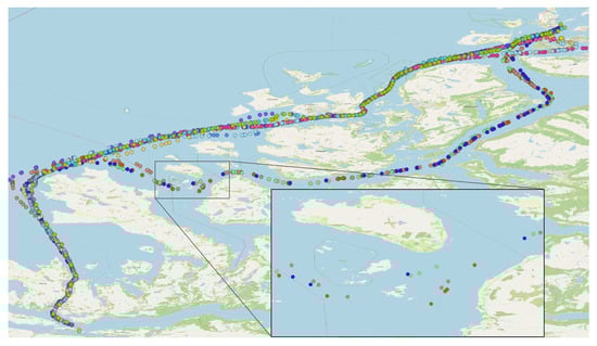
Figure 1.
Multiple trajectories of vessels between Ålesund and Måløy along the Norwegian coast. The dots represent AIS messages in a trajectory. Dots with the same color represent a single trajectory of a vessel. Observe the sparse AIS messages with irregular time intervals in all trajectories in a zoomed-in area. This area is surrounded by small and large islands. The sparse AIS messages in these trajectories pose a challenge for certain tasks in the maritime domain.
Once the representative trajectory between the two ports is estimated, the next task is to compute its waypoints, which provide information to the vessels related to changes in their dynamic features. A waypoint is the position in the AIS message-based trajectory where the vessel changes its course, speed, and possibly other dynamic-point features. A waypoint in the context of the present study is a pair of latitudes and longitudes that can be used by vessels to sail from one port to another. A sequence of waypoints with the minimum number of waypoints from one location (e.g., a port) to another is called a reference route. The goal of this paper is to estimate a reference route between two ports when AIS data are insufficient.
Estimating a representative trajectory and subsequently estimating its waypoints from historical AIS data in critical areas is challenging because vessels do not generally follow a fixed trajectory, precisely due to various reasons such as the size of the vessel, the effect of waves, and weather conditions, to name a few. Hence, trajectories are scattered over a vast navigable area, and estimating a reference route (a sequence of waypoints) becomes more challenging. Two approaches are typically followed in the maritime literature to detect a representative trajectory and its waypoints. (i) In the first approach, a representative aggregated trajectory is computed via, for example, density map information [11]. Here, the representative aggregated trajectory contains samples from multiple trajectories. Subsequently, waypoints of the aggregated trajectory are computed. The challenge with this approach is that the final reference route may not be smooth, owing to the sparse data and AIS messages selected from multiple distinct trajectories. As a result, it will not be feasible for vessels to sail, as the vessel would be redundantly required to change the course more often. Another challenge is that a large number of trajectories with high resolution are required for such an approach. (ii) In the second approach, the waypoints of all trajectories are individually computed and the estimated waypoints are clustered to detect common waypoints of trajectories [12]. Once clusters of waypoints are formed, selecting the center of the clusters becomes a challenge. Moreover, connecting the centers of clusters of waypoints is another significant challenge owing to safety issues, as the connecting lines may pass through un-sailable or restricted areas.
Considering the challenges mentioned above, we propose the following methodology for computing the reference route between two ports when the available data are sparse or insufficient. First, a single representative trajectory based on certain selection criteria, such as trajectories with high resolution in terms of AIS messages and maximum intersection/closeness with an average representative trajectory, is estimated. Then, the waypoints of a single representative trajectory are estimated. However, as previously discussed, the AIS messages typically exhibit a sporadic pattern in a single trajectory in a critical area, as illustrated in Figure 2; we considered the problem of detecting waypoints of a trajectory with missing or insufficient data. This study has focused on and investigated the problem of detecting waypoints for a given single trajectory with insufficient AIS messages, using various interpolation methods. Without interpolation, if we apply the waypoint estimation algorithm, the straight line in Euclidean space (and a great circle in the spherical geometry) connecting the two waypoints may pass through an unsafe area (e.g., land, shallow water). Even without any waypoint estimation, if we attempt to connect AIS messages via the straight line in Figure 2, it can sail through an area very close to land, which is not safe for the vessel.
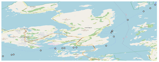
Figure 2.
An overview of sporadic AIS messages in the trajectory of a vessel in a critical area between Ålesund and Måløy along the Norwegian coast. The white dots represent the observed AIS messages. Observe that the AIS messages are recorded at irregular intervals and that the AIS messages are sparse along the route of the vessel.
In this paper, we mainly consider the problem of computing waypoints of a single representative trajectory that has insufficient AIS messages and passes through critical areas. The vessels in such critical areas do not have the flexibility to sail in wider routes due to regulations, shallow water, or islands. On the other hand, in the open sea, the task of computing waypoints from historical data is not a priority as the vessels have the flexibility to follow any path or direction. Waypoint estimation has been investigated in several studies, such as [13,14], and the interpolation of trajectories has been discussed in [15,16]. However, to the best of our knowledge, studies addressing the problem of interpolating a trajectory for waypoint estimation are scarce. This paper proposes a waypoint detection methodology for reference route estimation using the interpolation of AIS trajectories when the data between two locations—for example, ports—are sparse and inadequate.
The contributions of the present paper are as follows:
- An algorithm based on the multidimensional dynamic features of vessels for detecting waypoints of a single trajectory with missing or insufficient data using interpolation methods has been proposed. The proposed algorithm incorporates multiple motion features for the waypoint detection of an AIS-based trajectory.
- Various interpolation methods for improving the resolution of AIS message-based trajectories in critical areas have been investigated.
- Two types of waypoints are detected by the waypoint detection algorithm: waypoints on interpolated AIS messages and waypoints on observed AIS messages. To ensure safety, historical data can be used to replace interpolated waypoints with nearby AIS messages from the historical AIS data (or available true waypoints).
- Numerical results are presented that showcase the effectiveness of various interpolation methods before the waypoint detection algorithms are applied. Furthermore, numerical experiments provide a comparison of the proposed algorithm with an existing algorithm for waypoint detection.
The remainder of this paper is organized as follows: Section 2 discusses the works related to the considered problem in this paper and Section 3 describes the background information, such as definitions and interpolation methods for AIS trajectories. Section 4 presents an overview of the waypoints of the representative trajectory and its detection. The experimental evaluation of the proposed method is presented in Section 5 and conclusions are presented in Section 6.
2. Related Work
One of the main tasks toward achieving vessel awareness in the maritime domain is to estimate a representative trajectory and its waypoints based on historical data using, e.g., clustering algorithms, as proposed in [17,18]. Mostly, such clustering algorithms use various distance metrics [19] for finding the clusters in the data. A kernel density estimation-based method is proposed in [20] to estimate a representative trajectory for maritime traffic, and a verification method is presented. Another common approach is to build a network, often represented by a graph, where nodes denote the stops/waypoints and edges indicate the sailing route among nodes. Once a graph is constructed, graph-theory-based algorithms can be used to tackle estimation tasks, such as finding a path with the minimum number of waypoints between two ports [21]. Other works addressing the problem of building a maritime traffic route network from AIS historical data include [22,23,24].
The problem of waypoint detection has been addressed as a part of trajectory segmentation, for example, greedy Gaussian segmentation (GGS) [25], where the data in each segment are considered to originate from a multivariate Gaussian distribution. The proposed method computes the breakpoints of the segments and then estimates the parameters of each segment. The waypoint detection of AIS trajectories has been considered in several studies. For example, [13,14] presented waypoint detection methods for multiple trajectories to construct graphs with waypoints as nodes. Ref. [26] presented a lightweight algorithm called cumulative sum (CUSUM) to detect vessel maneuvering points. Moreover, [27] proposed a hybrid approach for detecting waypoints in streaming data scenarios. However, all these methods do not take into account the missing values in critical areas and apply methods of waypoint detection on trajectories with insufficient AIS messages, which can have missing values. The problem of insufficient AIS data has been investigated for various maritime domain tasks. A genetic-algorithm-based solution was proposed in [28] to extract a representative route using incomplete data. In addition, [29] dealt with incomplete data for recovering vessel trajectories using a tensor decomposition method. Various interpolation methods for AIS-based trajectories have been discussed in [16,30], as well as kinematic interpolation [15,31], Lagrange interpolation [32], and cubic Hermite spline interpolation [33]. Furthermore, the impact of interpolation on maritime anomaly detection was addressed in [34]. The problem of waypoint detection was considered in [35], where topographic information was included in the algorithm to avoid passing through land or restricted areas. In the next section, we present the background information, including several definitions and interpolation methods. Finally, [36] addresses the problem of low-quality AIS data using kinematic interpolation in a three-step approach consisting of data preprocessing, kinematic estimation, and error clustering. In [37], the authors propose a vessel pattern discovery approach from AIS data based on the clustering of waypoints. However, unlike our work, which targets waypoint detection, both proposed approaches are used in the context of anomaly detection.
3. Background
In this section, we present definitions of the concepts used to formulate the problem. These definitions also assist in explaining the different concepts presented in this paper.
3.1. Definitions
- Trajectory point: A minimal trajectory point () is defined as , where is the longitude of a moving object, is the latitude, and is the time that and were collected. is a set of features related to the motion of the vessel, such as course over the ground, speed over the ground, etc. is the identifier of a moving object, and is the set of all trajectory points. A trajectory point can include additional elements that represent the diverse features of a moving object in an application. The sequence of spatio-temporal points characterizes a trajectory.
- Trajectory: A trajectory is a time-ordered sequence of spatio-temporal points. A formal definition of a raw trajectory for a moving object o is given by , where . A trajectory can be split into smaller parts, called segments or sub-trajectories, which are defined next.
- Segment or Sub-Trajectory: A segment or sub-trajectory is a set of consecutive trajectory points between two waypoints belonging to a raw trajectory that represents a useful pattern or behavior of a moving object.
- Trajectory Point Feature: The trajectory point feature is an attribute that describes the state of a moving object. Examples of trajectory point features include the speed over ground, the course over ground, and acceleration. These features can be present in the observations of trajectory samples or computed from these observations. A combination of these point trajectory features can be exploited to detect the waypoints.
- True Waypoint: The true waypoint is a waypoint that maritime domain experts have manually placed by exploiting all the available information, such as navigation charts, regulations, and the history of navigation in the area.
3.2. Interpolation Methods
Various interpolation methods can be used to interpolate AIS-based trajectories. Interpolating AIS-based trajectories means interpolating the locations (pairs of latitude and longitude) as well as the dynamic features of the vessels, such as course over ground and speed over ground. Most of the tasks in maritime only require interpolating locations; certain tasks, such as waypoint detection, call for the interpolation of dynamic features. While errors introduced due to interpolating features do not pose any significant risk to the safety of vessels, interpolating locations requires attention, as the interpolated locations can be unsafe for vessels sailing through land, shallow water, or other restricted areas.
In this paper, we investigate the following types of interpolation for the interpolation of the AIS-messages-based trajectories for the task of waypoint detection.
3.2.1. Linear Interpolation
Linear interpolation is one of the simplest types of interpolation. Given two values, interpolating the third value between them is simply a point lying on the line connecting the two values. Let , denote the position (in one dimension) of a vessel at time and , respectively. Linear interpolation of position at that satisfies is given by
Similarly, other dynamic features, i.e., speed and course, can be interpolated linearly in the same manner. It is well known that linear interpolation is usually inadequate for interpolating AIS trajectories, as there can be large gaps between two AIS messages. Hence, other types of interpolation are used for the interpolation of AIS trajectories.
3.2.2. Cubic Spline Interpolation
Consider three points , , and for cubic spline interpolation purposes. We require to compute two piecewise cubic splines and to interpolate points among these given values, given by
where and are unknowns. Cubic spline interpolation can be computed by solving the following equations:
The remaining two equations are arbitrary, and some common options include boundary conditions such as natural splines, , and quadratic splines, . Some other types of interpolation methods involve other different options for the remaining equation.
3.2.3. Cubic Hermite Spline Interpolation
Suppose that we want to compute the cubic Hermite spline interpolation between two given points and . A cubic spline for is given by
where are unknowns. The derivative of is given by
Given the first derivative of evaluated at and , i.e., and , the cubic Hermite interpolation in interval is given by solving the following equations for :
We have four unknowns and four equations. Hence, there can be a solution. In the next section, we present the proposed methodology for the waypoint detection of a single representative trajectory with insufficient data.
4. Waypoint Detection in Sparse AIS Data
Thus far, we have introduced the background materials required for the proposed methodology. In this section, we present the main methodology for waypoint detection. First, we describe the model and problem formulation, followed by the proposed solution for the reference route detection and waypoint detection algorithm.
4.1. Model and Problem Formulation
We consider a model based on the multidimensional features of the trajectory points (defined in Section 3). Each trajectory point is mapped to an n-dimensional vector containing various dynamic features related to the motion of the vessel. The (n-dimensional) feature vector corresponding to trajectory point is given by , where is the course over the ground, is the speed over ground, and is the acceleration of the vessel. This is merely an instance of a feature vector that corresponds to a trajectory point. Some of these features are available in the observed trajectory samples, whereas others can be computed from observations. Because time and location information are not explicitly used for waypoint computation, we excluded time and location from the feature vector. The timestamp and location information, such as latitude and longitude, were used in the interpolation stage of the given trajectory.
Given a representative trajectory, i.e., a raw AIS message-based trajectory of a vessel, the goal is to compute its waypoints. Waypoints are locations where vessels change their dynamic features, such as the course over the ground and speed over the ground. However, in the present case, the AIS trajectory has missing values or insufficient data, which means that the waypoint detection algorithm cannot be directly applied to a given sparse trajectory. The problem statement is as follows: given a representative AIS message-based trajectory with insufficient data, compute the breakpoints in the course over ground and the speed of the vessel in the given trajectory. Leveraging these two features, we define a two-dimensional feature vector as , where d denotes the course over the ground, and v denotes the speed over the ground. Formally, given N samples of a trajectory, compute a set of waypoints , where is the i-th waypoint and K is the total number of waypoints such that there is a significant change in and/or with respect to its previous values.
4.2. Proposed Solution for Reference Route Detection Using Interpolation
To solve the problem of the waypoint detection of a representative trajectory with sparse data, a two-step solution is proposed in the present paper. In the first step, a given trajectory with insufficient AIS messages is interpolated using interpolation methods. In the next step, a waypoint detection algorithm is applied to the merged trajectory, which includes both interpolated and observed AIS messages, to estimate the waypoints. The various interpolation methods are introduced in Section 3.2. These interpolation methods are used to interpolate AIS messages in areas in which AIS messages are missing or insufficient for waypoint detection.
To detect waypoints in a single representative trajectory with insufficient data, we interpolate AIS messages along the trajectory and merge them with the observed messages. Subsequently, the waypoint detection algorithm is applied to the merged trajectory containing both the observed and interpolated AIS messages. The locations as well as the features are interpolated in order to apply a waypoint detection algorithm based on multidimensional features. The employed waypoint detection algorithm yields two types of waypoints: (i) waypoints sitting on observed AIS messages, and (ii) waypoints sitting on interpolated AIS messages. Because interpolated waypoints are not always guaranteed to be safe, they can be replaced by the closest nearby observed AIS message (or the true waypoint, if available) from the historical data. Thus, if two consecutive waypoints are not far away from each other, connecting them is safe in most cases in a critical area.
A flowchart of the methodology for reference route detection between the two ports considered in this paper is presented in Figure 3. As illustrated in the flowchart, the proposed methodology comprises several stages. First, trajectories based on AIS messages are retrieved between the two ports to compute a representative trajectory. When a representative trajectory is selected, the features of the given trajectory are computed in the next step, and the projection of the features to the 2D space is computed. Subsequently, interpolation methods are used to interpolate the trajectory features. After interpolation, a waypoint detection algorithm is applied to the merged trajectory. Finally, to improve the safety of the vessels, interpolated waypoints are replaced with possibly available true waypoints or historical AIS messages. Thus, a reference route, i.e., a sequence of waypoints, is obtained.
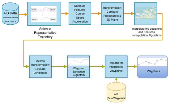
Figure 3.
Overall flowchart of the methodology of reference route estimation between two ports. The focus here is mainly on the waypoint detection together with the interpolation of the representative trajectory.
Next, we introduce the waypoint detection algorithm employed in this paper.
4.3. Waypoint Detection Algorithm
Given a representative trajectory between two locations, the goal is to estimate the waypoints of the trajectory such that, when connecting the waypoints, the connecting lines do not pass through a restricted or unsafe area (land, shallow water, regulated area, offshore platforms, marine life restricted areas, etc.). In this paper, we focus on waypoint detection using multiple dynamic features of maritime vessel trajectories. To this end, we employ a hybrid reactive buffering window (RBW) algorithm for the waypoint detection of a single representative trajectory with missing values or an insufficient number of AIS messages. Regarding the features involved in the decision of the waypoint, we are interested in the speed and course over the ground of the vessel, because these are the two main dynamic features that usually vary at waypoints. Additionally, if the course of a vessel is inaccurate, the speed can provide additional information regarding the waypoint.
| Algorithm 1 Waypoint Detection Using Hybrid Reactive Buffering Window (Hybrid RBW) Algorithm. |
| Input: Buffering window length w, distance threshold , variations threshold r, mean , and covariance |
| Output: A list of trajectory waypoints |
| Initialization: |
|
The underlying model considered in this study is based on the n-dimensional features of the trajectory points, which are mapped to an n-dimensional vector containing various features , as described in Section 4.1. Given trajectory feature vectors , we compute the set of waypoints , where . We assume that the feature vector follows a multidimensional Gaussian distribution, i.e., , where is the mean of the feature vector and is the covariance matrix of the feature vector. The probability density function of the multivariate Gaussian distribution is given by where denotes the determinant of the input matrix. We assume that the feature vector denoted by corresponding to the trajectory sample at the i-th time instant is an independent sample drawn from , and the multidimensional time series is partitioned into K segments. The k-th segment is identified by the parameters and of the Gaussian distribution.
In multidimensional feature-based waypoint detection, when the feature vector follows a Gaussian distribution, the goal is to estimate the locations of the changing points of the considered features, i.e., waypoints. There are available heuristic approaches, such as [25], that present a solution by solving the problem of multidimensional time-series segmentation. To make a decision about the trajectory sample regarding whether the trajectory point is a waypoint in a trajectory or not, we pose a detection problem: the null hypothesis () is that the present sample is a waypoint, whereas the alternate hypothesis () is that the present sample is not a waypoint, mathematically presented as and The underlying idea is that the feature vector follows the same distribution between the two waypoints. To determine a rule for deciding whether a trajectory sample belongs to a segment, we require a test statistic T for a threshold : . However, because the parameters (mean and covariance) are unknown, it is difficult to derive such test statistics. Therefore, we resort to heuristic approaches. In the case of multidimensional features, one of the most popular approaches is to use the Mahalanobis distance, given by , as a measure for hypothesis testing regarding whether the sample belongs to the Gaussian distribution . Observe that is a random variable. The probability distribution of is given by chi-squared with n degrees of freedom [38]. Given the number of features n and the confidence level, we can find the threshold for d such that a sample belongs to a given distribution. Specifically, in order to cover probability with an ellipsoid of radius d, we require , where is the upper percentile from the Chi-squared distribution with n degrees of freedom (see [38] Result 4.7 and [39]).
The waypoint detection algorithm–hybrid RBW is applied to the merged trajectory, which includes both observed and interpolated AIS messages. The interpolated features are the latitude, longitude, course over the ground, and speed over the ground. The overall hybrid RBW algorithm is presented in Algorithm 1. The algorithm works as follows. For each AIS message in a trajectory, it receives the trajectory point and computes its feature vector. If the number of samples is equal to the buffer length w, then the mean vector and sample covariance matrix of the feature vector are computed. However, to detect waypoints before the buffer is filled, the moving average of the previous feature vectors is compared to the current feature vector. Next, the Mahalanobis distance of the present feature vector is computed to compare it with a threshold. If the distance is larger than the threshold, it implies that the present feature vector is significantly different, and a waypoint is detected. This procedure is repeated for all samples of the given representative trajectory. Finally, a list of detected waypoints is produced as a result of the algorithm. In the next section, we present the numerical results based on real AIS data.
5. Experimental Evaluation
To numerically evaluate the proposed methodology for waypoint detection with insufficient data by exploiting interpolation methods, we have investigated the following research questions in this paper.
- RQ1. How do different interpolation methods perform during the prediction/fitting of AIS messages in vessel trajectories?
- RQ2. How do different interpolation methods affect the performance of the waypoint detection algorithms applied to trajectories with missing or insufficient AIS messages?
- RQ3. How does the proposed methodology perform when compared to other waypoint detection algorithms?
5.1. Maritime Datasets
In this paper, the AIS data used in the numerical experiments are owned and provided by Navtor, AS, Norway [40]. To evaluate the performance of waypoint detection methods, we require true labeled data in the form of a reference route, i.e., a sequence of true waypoints between two ports. To this end, we obtained the true waypoints of routes from a publicly available source, Routes and Route Information from the Norwegian Coastal Administration (NCA) [41]. It contains a collection of reference routes (a sequence of waypoints) among all the major ports in Norway. For example, two reference routes from Ålesund to Måløy, retrieved from the NCA website, are shown in Figure 4. These routes are safe and are recommended for sailing as they follow the local rules and regulations. Note that waypoints in critical areas are more frequent than in other areas, as vessels are required to change the direction of motion more often. Observe that the reference routes are merged into one common route in some areas. In addition, incoming and outgoing reference routes are predominantly different and they are required to have at least a minimum separation distance between them to ensure vessel safety.
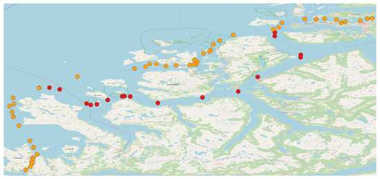
Figure 4.
Two one-way reference routes (true waypoints) from Ålesund to Måløy. Orange dots represent the northern route, while red dots represent the southern route. Note that these reference routes have common passage areas as they merge near the ports of Ålesund and Måløy.
5.2. Performance Evaluation Metrics
In this paper, we use the following metrics for the evaluation of the interpolation and waypoint detection methods.
- Mean Squared Error: To evaluate how well the interpolation methods can predict the missing AIS messages in a vessel trajectory, we utilize mean squared error (MSE), given bywhere is the true value, is the result of interpolation, and N is the total number of samples. In our case, for location interpolation, is a pair of latitude and longitude. MSE requires both the (true) observed AIS messages and the predicted AIS messages.
- Harmonic Mean of Purity and Coverage: Popular metrics for evaluating the performance of segmentation trajectories include purity and coverage. Purity and coverage were formally introduced as the evaluation criteria for segmentation algorithms [42]. We measured the purity and coverage of the estimated segments by comparing them with ground truth data. Purity shows the degree to which a trajectory segment is divided correctly compared with subject-matter expert segmentation. The coverage quantifies the extent to which the algorithm can cover the segments identified by a subject matter expert. Purity is mathematically defined as [42]where S is the set of segments discovered by the segmentation algorithm, is the set of labels provided by a subject-matter expert, k is the number of discovered waypoints, L is the number of expert labels, and is the number of trajectory points inside a segment with label . Coverage is defined as [42]where S is the set of segments discovered by the segmentation algorithm, is the set of segments by a subject-matter expert, is the number of trajectory points of the segment that belongs to the segment, and is the total number of points of the identified segment with a segment identifier equal to segment. The waypoints are treated as breakpoints of the segments. To generate labels inside the segments, we assign the same label (in this case, an integer) to all of the AIS messages between two waypoints. The highest possible value for both purity and coverage is 1.0, and the lowest possible value is 0. The perfect result will have both purity and coverage of 1.0. Since purity and coverage are two orthogonal metrics, we report the harmonic means of purity and coverage, given by , where P and C denote purity and coverage, respectively, to compare the performance of various algorithms [43]. A perfect result, where all the waypoints are correctly detected, would also obtain the harmonic mean of purity and coverage value of 1.
5.3. RQ 1: Performance of Interpolation Methods for Interpolating AIS Trajectories
The present paper is concerned with insufficient data in AIS trajectories for the task of waypoint detection and hence uses interpolation. Therefore, the goal of this research question is to evaluate different interpolation methods when interpolating AIS message-based trajectories.
- Experimental Setup. In order to evaluate the interpolation methods, we removed a number of AIS messages from the trajectories and then predicted these messages using various interpolation methods. Given the missing probability of an AIS message, each AIS message is uniformly selected for removal from the trajectory. It is pertinent to mention that the missing probability of an AIS message cannot be increased beyond a certain limit, as we cannot eliminate a large number of AIS messages from a trajectory and then interpolate the missing ones based on the remaining messages. MSE (defined in Equation (2)) is used to illustrate the performance of the interpolation methods. In this research question, the MSE values for all the methods are averaged across 50 trajectories.
- Results. A comparison of the performance of the interpolation methods, i.e., linear, cubic, and cubic Hermite interpolation, is shown in Figure 5. The MSE is presented against several missing probabilities of an AIS message in a trajectory. It can be observed for all the cases that when the missing probability increases, the MSE of the interpolation methods also exhibits an increasing trend. The cubic Hermite spline interpolation outperformed the other interpolation methods for lower values of missing probabilities. However, when the missing probability is increased beyond a certain limit, the MSE of the cubic Hermite interpolation method becomes higher than those of the linear and cubic interpolation methods. This is expected because interpolation methods require a reasonable amount of data to work properly, and they cannot work in scenarios when there are no adequate data available. This confirms that cubic Hermite interpolation can be used to interpolate AIS messages in the vessel trajectories. To corroborate this observation further, Figure 6 presents a comparison of how these interpolation methods perform while interpolating AIS message-based trajectories. Blue dots denote the observed AIS messages, whereas green, orange, and brown dots indicate cubic Hermite splines, cubic splines, and linear interpolation, respectively. Both linear and cubic spline interpolations can result in positions very close to the islands, whereas cubic Hermite splines yield interpolated locations comparatively in a safer area.
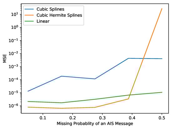 Figure 5. Mean square error of interpolation methods for different values of missing probability of an AIS message. The MSE for all the interpolation methods is averaged across 50 trajectories. The figure shows that cubic Hermite interpolation is appropriate for the interpolation of AIS message-based trajectories.
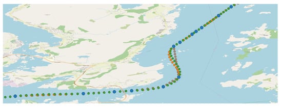 Figure 6. A comparison of the interpolation methods while interpolating a single trajectory in a critical area. Blue dots denote the observed AIS messages; green, orange, and brown represent cubic Hermite splines, cubic splines, and linear interpolation, respectively. Note that cubic Hermite spline interpolation yields safer interpolated AIS messages as compared to linear and cubic spline interpolation.
5.4. RQ2: Interpolation Methods’ Effects on the Waypoint Detection Algorithm
This research question aims to evaluate the effect of interpolation on the waypoint detection task. The main idea of this paper is to use interpolation when the representative trajectory contains an inadequate number of AIS messages. Hence, we evaluate and compare different interpolation methods for waypoint detection.
- Experimental Setup. To answer this research question, we exploited the true labeled data. The true waypoints of a reference route between Ålesund and Måløy were used to evaluate the performance of the proposed methodology for waypoint detection. True labeled data were generated as follows. Given the interpolated trajectory and true waypoints, the closest AIS message in the interpolated trajectory to the true waypoint of the NCA reference route is labeled as a true waypoint of the given interpolated trajectory. This procedure is followed because the given representative trajectory is not exactly the same as the NCA reference route. Hence, the estimated waypoints of the representative route will lie in the vicinity of the NCA true waypoints. To evaluate the performance, we assign the label of true waypoints to the AIS messages along the representative interpolated merged trajectory based on the minimum distance. To illustrate this further, we display an overview of the observed AIS messages, true waypoints from the NCA reference route, estimated waypoints, and labeled waypoints for each representative trajectory containing both the observed and interpolated AIS messages in one area in Figure 7. As discussed, if the representative trajectory closely follows the true waypoints, then the labeled waypoints will also be closer to the true waypoints. In this case, in Figure 7, the representative trajectory of the vessel is following the true waypoints or the true reference route near the bridge but not closely following it in other areas. Consequently, in an area where the representative route follows the true reference route, the labeled waypoints are closer to the true waypoints from the NCA route, compared to areas where the representative trajectory is at a distance from the NCA reference route.
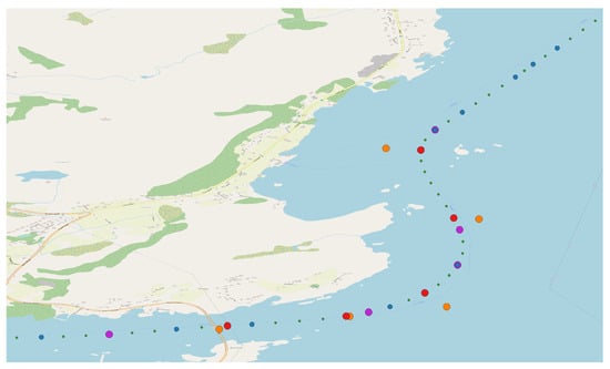 Figure 7. An overview of the observed AIS messages, interpolated AIS messages, true waypoints from the NCA reference route, and the labeled waypoints for each representative trajectory, which are required for the evaluation of the waypoint detection algorithm. Blue dots: observed AIS messages; green dots: interpolated AIS messages; orange dots: true waypoints from the NCA reference route; purple dots: waypoints estimated by the hybrid RBW; red dots: labeled waypoints that are part of the merged trajectory but closest to the true waypoints.
 - Results. The numerical results are presented in Figure 8; performance in terms of the harmonic mean of purity and coverage for the waypoint detection algorithm with various covariance estimators is shown. True labels were manually generated by observing the interpolated trajectory. Different covariance estimators, i.e., shrunk covariance [44], Oracle Approximating Shrinkage (OAS) [44], minimum covariance determinant [45], elliptical envelope [46], and Ledoit-Wolf [47] estimators, have been tested to be used in hybrid RBW for covariance estimation. These are different covariance estimators with diverse properties. The figure demonstrates that all these estimators have almost the same performance in terms of the harmonic mean of purity and coverage. However, the shrunk covariance estimator has a slightly higher harmonic mean of purity and coverage than the other covariance estimators. Moreover, a comparison of the different interpolation methods for waypoint detection performance in the form of the harmonic mean of purity and coverage is illustrated in Figure 9. The figure demonstrates that cubic Hermite interpolation is suitable for waypoint detection when the (representative) trajectory contains insufficient AIS messages. Finally, to have an overview of the waypoint estimation for a representative trajectory, a comparison of the true and estimated waypoints is presented in Figure 10. It can be observed that the estimated waypoints mostly match the locations of the true waypoints. The true waypoints were manually selected according to the trajectory. The trajectory was interpolated using cubic Hermite spline interpolation.
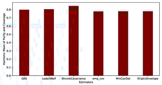 Figure 8. For a single AIS trajectory, harmonic means of purity and coverage for different estimators are presented. Cubic Hermite spline interpolation is used for this experiment. The estimated waypoints are compared to true waypoints for this experiment.
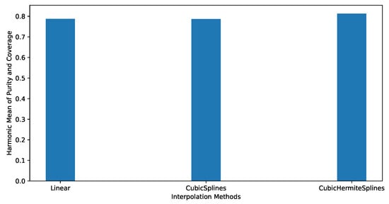 Figure 9. Harmonic of purity and coverage when the representative trajectory is interpolated by using different interpolation methods before applying the waypoint detection method. A comparison of the performance of interpolation methods for the waypoint detection task.
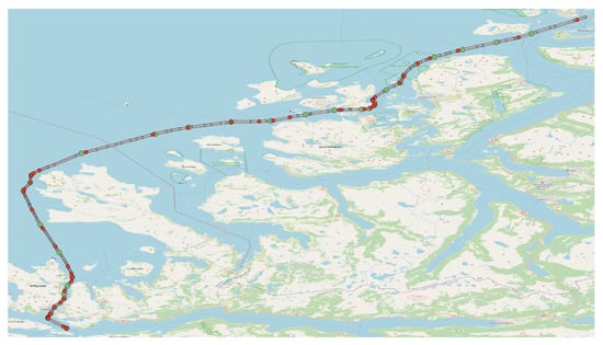 Figure 10. Screenshot of a representative trajectory, estimated waypoints, and the manually selected true waypoints between Ålesund and Måløy. The green dots represent the estimated waypoints, and the red dots represent the manually selected true waypoints. Firstly, the trajectory is interpolated via cubic Hermite spline interpolation and, then, the waypoint estimation algorithm is applied to the merged trajectory containing both interpolated AIS messages and the observed AIS messages. Note that the estimated waypoints are, most of the time, nearby in the vicinity of the true waypoints.
5.5. RQ3: Comparison with Other Waypoint Detection Algorithms
Comparing the proposed methodology for reference route estimation having insufficient AIS data with other algorithms is important. Hence, this research question is dealing with a comparison of the proposed methodology for waypoint detection with other available methods.
- Experimental Setup. We consider a comparison with the CUSUM algorithm [48] applied to the dynamic feature of course over ground. We used the implementation of CUSUM available in [49]. The waypoints of a representative trajectory with inadequate AIS messages are detected. The same interpolation method (i.e., cubic Hermite interpolation) is used for both waypoint detection algorithms.
- Results. Figure 11 compares the proposed method and the commonly known benchmark CUSUM algorithm for waypoint detection. This result is based on the representative trajectory between Ålesund and Måløy. The hyperparameters of CUSUM are tuned such that a high harmonic mean of purity and coverage is obtained. Similarly, the hyperparameters of hybrid RBW are also selected so that a high value of the harmonic mean of purity and coverage is produced. The proposed method has a higher harmonic mean of purity and coverage (0.82) than that of the CUSUM algorithm (0.79); hence, the proposed algorithm outperforms CUSUM in the envisaged scenario for the waypoint detection of a trajectory with sparse data.
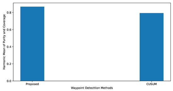 Figure 11. Harmonic mean of purity and coverage vs. waypoint detection algorithms. A comparison of the waypoint detection algorithm in terms of the harmonic mean of purity and coverage. Interpolation period = 60 s.
5.6. Discussion of the Results
We have presented the results of the numerical experiments; however, it is essential to bear in mind that the task of waypoint detection with insufficient data poses various challenges. The results show that cubic Hermite interpolation performs better than other interpolation methods; however, this does not imply that this will always be the case. Cubic Hermite interpolation can also yield interpolated AIS messages in an unsafe area when, for instance, the number of available AIS messages in a trajectory is insufficient. In addition to instability in the results of interpolation methods, the waypoint detection algorithm can miss a potential waypoint or somehow estimate the location of the waypoint with inconsistencies. Furthermore, both incoming and outgoing reference routes generated by the proposed methodology using a single representative trajectory can also be problematic. This is because the estimated reference routes are approximately accurate, and there is usually a very subtle separation between the two routes. Owing to the inaccuracies introduced by interpolation and the waypoint estimation algorithm, there is a possibility that the resulting incoming and outgoing reference routes are unreliable and cannot be followed precisely. The goal of the proposed methodology is to provide a tool for recommendations regarding the reference routes between the two ports to the crew onboard the vessel. Ideally, there would be a universal testing system available to determine whether the provided reference route is safe and according to the maritime regulations in the area. However, this type of testing setup is usually unavailable globally owing to its numerous intricacies. Hence, all these results and discussions reveal that these challenges should be kept in mind for the task of waypoint detection with insufficient AIS data.
6. Conclusions
We propose a methodology for estimating a reference route, which includes estimating a representative trajectory and its waypoints, for a scenario in which the available AIS data between two locations are sparse and insufficient. Interpolation methods were used to tackle the problem of missing values along the trajectory. Three interpolation methods, linear interpolation, cubic spline interpolation, and cubic Hermite spline interpolation, were used and compared in interpolating AIS messages in a trajectory with insufficient data. A waypoint estimation algorithm was presented to estimate the waypoints of the interpolated representative trajectory. The proposed algorithm was experimentally evaluated on a maritime dataset covering the geographic area between Ålesund and Måløy in Norway. The experimental results demonstrated that the proposed methodology is effective in the considered scenario of waypoint detection in sparse AIS data, compared to the existing approaches for waypoint detection, such as CUSUM. The proposed waypoint estimation approach can be used when creating vessel passage plans (consisting of waypoints), which are often created manually and can therefore be prone to errors or require great effort from ship operators.
6.1. Limitations
There are several limitations of the present methodology. First of all, the proposed algorithm has several hyperparameters, which are required to be tuned. Moreover, finding the optimal interpolation time period is also a challenging task for an application. As discussed in Section 5.6, a perfectly safe approach cannot be guaranteed when the AIS data are insufficient.
6.2. Future Work
In future work, we will improve the safety and accuracy of the estimated reference route by incorporating information from alternative sources of data, such as weather information, local regulations, and historical data about the incidents in maritime, to name a few. Furthermore, we will evaluate the proposed approach on additional datasets containing even more sparse AIS messages than the dataset used in the current paper.
Author Contributions
Conceptualization, B.Z., D.M., and T.K.; methodology, B.Z. and D.M.; software, B.Z.; validation, B.Z., D.M. and T.K.; formal analysis, B.Z., D.M. and T.K.; investigation, B.Z.; resources, D.M. and T.K.; data curation, T.K.; writing—original draft preparation, B.Z. and D.M.; writing—review and editing, B.Z., D.M. and T.K.; visualization, B.Z.; supervision, D.M.; project administration, D.M.; funding acquisition, D.M. All authors have read and agreed to the published version of the manuscript.
Funding
This work is supported by ECSEL JU under grant agreement No. 101007260 and the Research Council of Norway under grant agreement No. 329090.
Institutional Review Board Statement
Not applicable.
Informed Consent Statement
Not applicable.
Data Availability Statement
Restrictions apply to the availability of these data. Data were obtained from Navtor, AS, Norway.
Acknowledgments
The authors of the paper would like to thank Joachim Berdal Haga, Chief Research Engineer at Simula, for helping with the code for this work.
Conflicts of Interest
The authors declare no conflict of interest.
Abbreviations
The following abbreviations are used in this manuscript:
| AIS | Automatic identification system |
| CUSUM | Cumulative sum |
| GGS | Greedy Gaussian segmentation |
| IMO | International Maritime Organization |
| MSE | Mean squared error |
| NCA | Norwegian Coastal Administration |
| RBW | Reactive buffering window |
References
- Le Tixerant, M.; Le Guyader, D.; Gourmelon, F.; Queffelec, B. How can Automatic Identification System (AIS) data be used for maritime spatial planning? Ocean Coast. Manag. 2018, 166, 18–30. [Google Scholar] [CrossRef]
- Tu, E.; Zhang, G.; Rachmawati, L.; Rajabally, E.; Huang, G.B. Exploiting AIS Data for Intelligent Maritime Navigation: A Comprehensive Survey From Data to Methodology. IEEE Trans. Intell. Transp. Syst. 2018, 19, 1559–1582. [Google Scholar] [CrossRef]
- Lee, E.; Mokashi, A.J.; Moon, S.Y.; Kim, G. The Maturity of Automatic Identification Systems (AIS) and Its Implications for Innovation. J. Mar. Sci. Eng. 2019, 7, 287. [Google Scholar] [CrossRef]
- Dominguez, A.G. Smart Ships: Mobile Applications, Cloud and Big Data on Marine Traffic for Increased Safety and Optimized Costs Operations. In Proceedings of the International Conference on Artificial Intelligence, Modelling and Simulation, Madrid, Spain, 18–20 November 2014; pp. 303–308. [Google Scholar]
- Claramunt, C.; Ray, C.; Salmon, L.; Camossi, E.; Hadzagic, M.; Jousselme, A.; Andrienko, G.; Andrienko, N.; Theodoridis, Y.; Vouros, G. Maritime data integration and analysis: Recent progress and research challenges. Adv. Database Technol. EDBT 2017, 2017, 192–197. [Google Scholar]
- Last, P.; Bahlke, C.; Hering-Bertram, M.; Linsen, L. Comprehensive analysis of automatic identification system (AIS) data in regard to vessel movement prediction. J. Navig. 2014, 67, 791–809. [Google Scholar] [CrossRef]
- Kontopoulos, I.; Chatzikokolakis, K.; Zissis, D.; Tserpes, K.; Spiliopoulos, G. Real-time maritime anomaly detection: Detecting intentional AIS switch-off. Int. J. Big Data Intell. 2020, 7, 85–96. [Google Scholar] [CrossRef]
- Mazzarella, F.; Vespe, M.; Alessandrini, A.; Tarchi, D.; Aulicino, G.; Vollero, A. A novel anomaly detection approach to identify intentional AIS on-off switching. Expert Syst. Appl. 2017, 78, 110–123. [Google Scholar] [CrossRef]
- Ray, C.; Gallen, R.; Iphar, C.; Napoli, A.; Bouju, A. DeAIS project: Detection of AIS spoofing and resulting risks. In Proceedings of the OCEANS, Genova, Italy, 18–21 May 2015; pp. 1–6. [Google Scholar]
- Ikonomakis, A.; Nielsen, U.D.; Holst, K.K.; Dietz, J.; Galeazzi, R. Validation and correction of auto-logged position measurements. Commun. Transp. Res. 2022, 2, 100051. [Google Scholar] [CrossRef]
- Wu, L.; Xu, Y.; Wang, Q.; Wang, F.; Xu, Z. Mapping global shipping density from AIS data. J. Navig. 2017, 70, 67–81. [Google Scholar] [CrossRef]
- Onyango, S.O.; Owiredu, S.A.; Kim, K.I.; Yoo, S.L. A Quasi-Intelligent Maritime Route Extraction from AIS Data. Sensors 2022, 22, 8639. [Google Scholar] [CrossRef]
- Arguedas, V.F.; Pallotta, G.; Vespe, M. Maritime traffic networks: From historical positioning data to unsupervised maritime traffic monitoring. IEEE Trans. Intell. Transp. Syst. 2017, 19, 722–732. [Google Scholar] [CrossRef]
- Vespe, M.; Visentini, I.; Bryan, K.; Braca, P. Unsupervised learning of maritime traffic patterns for anomaly detection. In Proceedings of the IET Data Fusion & Target Tracking Conference: Algorithms & Applications, London, UK, 16–17 May 2012. [Google Scholar]
- Long, J.A. Kinematic interpolation of movement data. Int. J. Geogr. Inf. Sci. 2016, 30, 854–868. [Google Scholar] [CrossRef]
- Nguyen, V.S.; Im, N.k.; Lee, S.m. The interpolation method for the missing AIS data of ship. J. Navig. Port Res. 2015, 39, 377–384. [Google Scholar] [CrossRef]
- Lee, J.S.; Lee, H.T.; Cho, I.S. Maritime Traffic Route Detection Framework Based on Statistical Density Analysis From AIS Data Using a Clustering Algorithm. IEEE Access 2022, 10, 23355–23366. [Google Scholar] [CrossRef]
- Zygouras, N.; Spiliopoulos, G.; Zissis, D. Detecting representative trajectories from global AIS datasets. In Proceedings of the IEEE International Intelligent Transportation Systems Conference (ITSC), Indianapolis, IN, USA, 19–22 September 2021; pp. 2278–2285. [Google Scholar]
- Besse, P.C.; Guillouet, B.; Loubes, J.M.; Royer, F. Review and perspective for distance-based clustering of vehicle trajectories. IEEE Trans. Intell. Transp. Syst. 2016, 17, 3306–3317. [Google Scholar] [CrossRef]
- Lee, J.S.; Son, W.J.; Lee, H.T.; Cho, I.S. Verification of novel maritime route extraction using kernel density estimation analysis with automatic identification system data. J. Mar. Sci. Eng. 2020, 8, 375. [Google Scholar] [CrossRef]
- Silveira, P.; Teixeira, A.; Guedes-Soares, C. AIS based shipping routes using the Dijkstra algorithm. TransNav Int. J. Mar. Navig. Saf. Sea Transp. 2019, 13, 565–571. [Google Scholar] [CrossRef]
- Lei, P.R.; Tsai, T.H.; Peng, W.C. Discovering maritime traffic route from AIS network. In Proceedings of the Asia-Pacific Network Operations and Management Symposium (APNOMS), Kanazawa, Japan, 5–7 October 2016; pp. 1–6. [Google Scholar]
- Wang, G.; Meng, J.; Han, Y. Extraction of maritime road networks from large-scale AIS data. IEEE Access 2019, 7, 123035–123048. [Google Scholar] [CrossRef]
- Zhang, S.K.; Shi, G.Y.; Liu, Z.J.; Zhao, Z.W.; Wu, Z.L. Data-driven based automatic maritime routing from massive AIS trajectories in the face of disparity. Ocean Eng. 2018, 155, 240–250. [Google Scholar] [CrossRef]
- Hallac, D.; Nystrup, P.; Boyd, S. Greedy Gaussian segmentation of multivariate time series. Adv. Data Anal. Classif. 2019, 13, 727–751. [Google Scholar] [CrossRef]
- Lamm, A.; Hahn, A. Detecting maneuvers in maritime observation data with CUSUM. In Proceedings of the IEEE International Symposium on Signal Processing and Information Technology (ISSPIT), Bilbao, Spain, 18–20 December 2017; pp. 122–127. [Google Scholar]
- Dobrkovic, A.; Iacob, M.E.; Van Hillegersberg, J. Using machine learning for unsupervised maritime waypoint discovery from streaming AIS data. In Proceedings of the Proceedings of the International Conference on Knowledge Technologies and Data-driven Business, Graz, Austria, 18–21 October 2015; pp. 1–8. [Google Scholar]
- Dobrkovic, A.; Iacob, M.E.; van Hillegersberg, J. Maritime pattern extraction and route reconstruction from incomplete AIS data. Int. J. Data Sci. Anal. 2018, 5, 111–136. [Google Scholar] [CrossRef]
- Liu, C.; Chen, X. Vessel track recovery With incomplete AIS data using tensor CANDECOM/PARAFAC decomposition. J. Navig. 2014, 67, 83–99. [Google Scholar] [CrossRef]
- Jie, X.; Chaozhong, W.; Zhijun, C.; Xiaoxuan, C. A novel estimation algorithm for interpolating ship motion. In Proceedings of the International Conference on Transportation Information and Safety (ICTIS), Banff, AB, Canada, 8–10 August 2017; pp. 557–562. [Google Scholar]
- Guo, S.; Mou, J.; Chen, L.; Chen, P. Improved kinematic interpolation for AIS trajectory reconstruction. Ocean Eng. 2021, 234, 109256. [Google Scholar] [CrossRef]
- Kontopoulos, I.; Varlamis, I.; Tserpes, K. A distributed framework for extracting maritime traffic patterns. Int. J. Geogr. Inf. Sci. 2021, 35, 767–792. [Google Scholar] [CrossRef]
- Zhang, D.; Li, J.; Wu, Q.; Liu, X.; Chu, X.; He, W. Enhance the AIS data availability by screening and interpolation. In Proceedings of the International Conference on Transportation Information and Safety (ICTIS), Banff, AB, Canada, 8–10 August 2017; pp. 981–986. [Google Scholar]
- Abreu, F.H.; Soares, A.; Paulovich, F.V.; Matwin, S. A trajectory scoring tool for local anomaly detection in maritime traffic using visual analytics. ISPRS Int. J. Geo-Inf. 2021, 10, 412. [Google Scholar] [CrossRef]
- Lee, W.; Cho, S.W. AIS Trajectories Simplification Algorithm Considering Topographic Information. Sensors 2022, 22, 7036. [Google Scholar] [CrossRef] [PubMed]
- Guo, S.; Mou, J.; Chen, L.; Chen, P. An Anomaly Detection Method for AIS Trajectory Based on Kinematic Interpolation. J. Mar. Sci. Eng. 2021, 9, 609. [Google Scholar] [CrossRef]
- Pallotta, G.; Vespe, M.; Bryan, K. Vessel Pattern Knowledge Discovery from AIS Data: A Framework for Anomaly Detection and Route Prediction. Entropy 2013, 15, 2218–2245. [Google Scholar] [CrossRef]
- Johnson, R.A.; Wichern, D.W. Applied Multivariate Statistical Analysis; Prentice Hall: Upper Saddle River, NJ, USA, 2014; Volume 6. [Google Scholar]
- Bajorski, P. Statistics for Imaging, Optics, and Photonics; John Wiley & Sons: Hoboken, NJ, USA, 2011; Volume 808. [Google Scholar]
- Available online: https://navtor.com/ (accessed on 2 March 2023).
- Available online: https://routeinfo.no/ (accessed on 2 March 2023).
- Soares Júnior, A.; Moreno, B.N.; Times, V.C.; Matwin, S.; Cabral, L.d.A.F. GRASP-UTS: An algorithm for unsupervised trajectory segmentation. Int. J. Geogr. Inf. Sci. 2015, 29, 46–68. [Google Scholar] [CrossRef]
- Etemad, M. Novel Algorithms for Trajectory Segmentation Based on Interpolation-Based Change Detection Strategies. Ph.D. Thesis, Dalhousie University, Halifax, NS, Canada, 2020. [Google Scholar]
- Chen, Y.; Wiesel, A.; Eldar, Y.C.; Hero, A.O. Shrinkage Algorithms for MMSE Covariance Estimation. IEEE Trans. Signal Process. 2010, 58, 5016–5029. [Google Scholar] [CrossRef]
- Rousseeuw, P.J. Least median of squares regression. J. Am. Stat. Assoc. 1984, 79, 871–880. [Google Scholar] [CrossRef]
- Rousseeuw, P.J.; Driessen, K.V. A fast algorithm for the minimum covariance determinant estimator. Technometrics 1999, 41, 212–223. [Google Scholar] [CrossRef]
- Ledoit, O.; Wolf, M. A well-conditioned estimator for large-dimensional covariance matrices. J. Multivar. Anal. 2004, 88, 365–411. [Google Scholar] [CrossRef]
- Gustafsson, F.; Gustafsson, F. Adaptive Filtering and Change Detection; Wiley: New York, NY, USA, 2000; Volume 1. [Google Scholar]
- Duarte, M. Detecta: A Python Module to Detect Events in Data. Available online: https://github.com/demotu/detecta (accessed on 2 March 2023).
Disclaimer/Publisher’s Note: The statements, opinions and data contained in all publications are solely those of the individual author(s) and contributor(s) and not of MDPI and/or the editor(s). MDPI and/or the editor(s) disclaim responsibility for any injury to people or property resulting from any ideas, methods, instructions or products referred to in the content. |
© 2023 by the authors. Licensee MDPI, Basel, Switzerland. This article is an open access article distributed under the terms and conditions of the Creative Commons Attribution (CC BY) license (https://creativecommons.org/licenses/by/4.0/).