Article

Research on Underwater Image Restoration Technology Based on Multi-Domain Translation

1
School of Information Science and Engineering, University of Jinan, Jinan 250022, China
2
Shandong Provincial Key Laboratory of Network-Based Intelligent Computing, Jinan 250022, China
3
School of Information Science and Engineering, Chongqing Jiaotong University, Chongqing 400074, China
*
Authors to whom correspondence should be addressed.
J. Mar. Sci. Eng. 2023, 11(3), 674; https://doi.org/10.3390/jmse11030674
Submission received: 22 February 2023 / Revised: 18 March 2023 / Accepted: 20 March 2023 / Published: 22 March 2023
(This article belongs to the Special Issue Advances in Underwater Robots for Intervention)

Abstract

:
Underwater images are crucial in various underwater applications, including marine engineering, underwater robotics, and subsea coral farming. However, obtaining paired data for these images is challenging due to factors such as light absorption and scattering, suspended particles in the water, and camera angles. Underwater image recovery algorithms typically use real unpaired dataset or synthetic paired dataset. However, they often encounter image quality issues and noise labeling problems that can affect algorithm performance. To address these challenges and further improve the quality of underwater image restoration, this work proposes a multi-domain translation method based on domain partitioning. Firstly, this paper proposes an improved confidence estimation algorithm, which uses the number of times a sample is correctly predicted in a continuous period as a confidence estimate. The confidence value estimates are sorted and compared with the real probability to continuously optimize the confidence estimation and improve the classification performance of the algorithm. Secondly, a U-net structure is used to construct the underwater image restoration network, which can learn the relationship between the two domains. The discriminator uses full convolution to improve the performance of the discriminator by outputting the true and false images along with the category to which the true image belongs. Finally, the improved confidence estimation algorithm is combined with the discriminator in the image restoration network to invert the labels for images with low confidence values in the clean domain as images in the degraded domain. The next step of image restoration is then performed based on the new dataset that is divided. In this way, the multi-domain conversion of underwater images is achieved, which helps in the recovery of underwater images. Experimental results show that the proposed method effectively improves the quality and quantity of the images.

1. Introduction

The study and application of marine resources is crucial aspect of the academic field of human development. The use of Autonomous Underwater Vehicles (AUVs) has emerged as a significant tool for exploring and studying marine resources, particularly in marine development and coastal defense. The visual information collected by the AUV’s vision system plays a pivotal role in detecting and understanding the underwater environment. However, due to challenges posed by light absorption and scattering in underwater environments, images captured by AUVs often suffer from blurring and color degradation. To address these issues, numerous academic methods have been proposed, which are broadly categorized into three approaches: the first is based on the Jaffe–McGlamery underwater imaging model [1,2,3], the second is based on the dark channel prior (DCP) [4,5,6], and the third is based on deep learning methods. In recent years, the field of computer vision has seen significant advancements in the application of deep learning, which make it a highly effective tool for addressing underwater image problems in the academic realm.
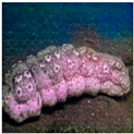
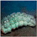
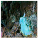
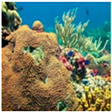
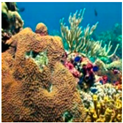
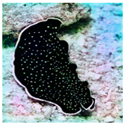
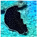
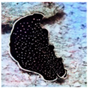
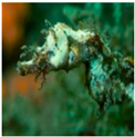
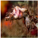
For deep learning methods, data is crucial, and high-quality datasets can significantly enhance the efficacy of model training. However, obtaining the paired real datasets for underwater image acquisition poses a significant challenge. As a result, unpaired real datasets are often obtained using subjective methods [7] or a combination of subjective and objective [8] division methods. Unfortunately, such division methods can lead to poor-quality datasets, which are shown in Figure 1.
In Figure 1c,d are both in the clean domain, but their clarity differs, with (c) being of poor quality. Most of the current research on underwater image restoration employs synthetic datasets, which are categorized as paired and unpaired. The SUID dataset [9] and the Li dataset [10] synthesize underwater images using ground truth images. Moreover, the proposed Cyclic Consistency Network (CycleGAN) [11] addresses the issue of the paired dataset’s unavailability. Cycle consistency enables the conversion of images between two distinct domains. For EUVP’s paired dataset, CycleGAN uses real underwater images to obtain reduced ground truth. On the other hand, UGAN [12] and UFO-120 [13] use CycleGAN to generate distorted underwater datasets based on real ground images. The degraded images in the UIEB [14] dataset were real underwater images, while the ground truth was obtained from various conventional methods. The UUIE [15] dataset is unpaired and comprises images from EUVP and UIEB datasets, as well as some high-quality in-air images in this dataset from ImageNet [16] or that were collected from the internet. Paired synthetic datasets were generated after processing using several algorithms. It is crucial to note that there exists a difference in data distribution between synthetic and real data, which leads to variations in training results.
For classification tasks for deep learning, validating a model not only requires correct predictions, but also requires an awareness of the confidence level during the predictions. Overconfident predictions can make the network model unreliable; hence, there is the need to address this issue. Moon et al. [17] proposed a solution by training deep neural networks using a novel loss function named Correctness Ranking Loss. This method regularizes class probabilities to provide a better confidence estimate by ranking them based on the ordinal number of confidence estimation. However, as the number increases in the training epoch, the ranking process changes steadily and successively, and subsequent sequential numerical rankings do not work.
When the data distributions of the source and target domains differ but the tasks are the same, domain adaptation enables the interconversion between different domains and utilizes information-rich source domain samples to improve the performance of the target domain model. The success of Generative Adversarial Networks (GANs) [18] in the field of image-to-image translation [19] provides a feasible approach to performing image translation between two or more domains in an unsupervised manner. While traditional GAN networks are unidirectional, CycleGAN [11] consists of two mirror-symmetric GANs that form a ring network. The purpose of this model is to learn the mapping relationship from the original input to the target domain from the source domain. In recent years, CycleGAN and its modifications have successfully restored underwater images using synthetic paired datasets for training [20,21,22,23]. Unpaired datasets were also used for training [24,25]. During GAN training, pattern collapse is prone to occur, which leads to high image degradation when the image orientation changes. This degradation is not ideal for underwater image datasets. CycleGAN utilizes cycle consistency to achieve conversion between two domains, but for domains that number more than two, more than one model needs to be learned. The StarGAN [26] proposal solves the multi-domain problem by using only one model to translate between different domains.
Taking inspiration from StarGAN and considering the variations in the quality of underwater image datasets, the objective of this work is to partition the dataset and conduct training in several domains to accomplish the restoration of underwater images. First, an improved confidence estimation algorithm is proposed for the dataset classification process. The algorithm attends to the current state of each sample to capture the dynamic changes in the network. It uses the frequency of consecutive correctly predicted samples during the training process as the probability of correctness, which is ranked with the confidence estimate to obtain reliable predictions. Secondly, an image restoration network with an auxiliary classifier in the discriminator is built. The auxiliary classifier can output the class of the image based on the judgment of whether the image is true or false. Lastly, the improved confidence estimation algorithm is combined with the image restoration network discriminator to improve the classification performance of the dataset. On the one hand, the improved confidence estimation algorithm can obtain the confidence value of the sample, and use the inversion label of the sample with a low confidence value in the clean domain as the distorted domain to classify the image. On the other hand, the ability of the discriminator to discriminate between true and false images is also enhanced. This restores the distorted underwater images and enhances their visual quality. The subsequent sections of this academic paper are structured as follows: The methodology is described in detail in Section 2. The experimental results, along with quantitative and qualitative evaluations, are presented in Section 3. Finally, Section 4 presents the conclusion and potential avenues for future research.

2. Proposed Method

This section presents the details of multi-domain translation in this work. The proposed improved confidence estimation method is first described in Section 2.1. Then, Section 2.2 describes the details of the multi-domain translation network module, including the network module used for training and the loss function.

2.1. Confidence Estimation Improvement Method

In accordance with [17], the authors proposed a new method of training deep neural networkswith a novel loss function, called Correctness Ranking Loss, which regularizes class probabilities to be better confidence estimates in terms of ordinal ranking according to confidence. The authors’ proposed method is easy to implement and can be applied to existing architectures without any modification. The Correctness Ranking Loss L C R function proposed by the authors is shown in Equation (1).
L C R x i , x j = max ( 0 , g c i , c j k i k j + | c i c j | )
In (1), for a pair of x i and x j , c i and c j are the proportion of correct events of x i over the total number of examinations (i.e., c i ), and k i , k j represent the confidence of each sample, respectively. | c i c j | represents margin. For a pair with c i > c j , the CRL will be zero when k i is larger than k j + | c i c j | , but, otherwise, a loss will be incurred. g c i , c j is shown in Equation (2).
g c i , c j = 1 ,         i f   c i > c j 0 ,         i f   c i = c j 1 ,         o t h e r w i s e
The method in this paper is to add a coefficient in front of | c i c j | , as is shown in Equations (3) and (4).
L C R x i , x j = max 0 , g c i , c j k i k j + λ c i c j
λ = 1 1 2 n
In Equations (3) and (4), n represents the number of consecutive correct predictions on a sample, and λ is expressed as the stability of correct predictions. Specifically, assume that “×” represents that the classifier predicts the sample label incorrectly, and “√” represents that the classifier predicts the sample label correctly. Then, if the history of continuous judgment is [×], then λ = 0 ; if the history of continuous judgment is [×√], then λ = 1 ( 1 2 ) 1 ; if the history of continuous judgment is [×√√], then λ = 1 ( 1 2 ) 2 ; if the history of judgment is [×√√××√√√], then λ = 1 ( 1 2 ) 3 . The purpose is that the more consecutive correct times there are, the higher the confidence. Therefore, the improved algorithm takes the number of consecutive correct predictions of samples during training as a coefficient to obtain a good confidence estimation in terms of ordinal ranking according to confidence to obtain more accurate predictions.
During extended periods of training in the deep neural network, the network’s state is constantly changing, thus resulting in dynamic shifts in the network’s evaluation of the samples. In the later stages of training, the confidence estimation may not change significantly. So, unlike Moon’s method, the purpose of the improvement is to emphasize the current state of the sample rather than its historical state, which is more indicative of the network’s current performance. This is accomplished by pushing the number of correct predictions from the back to the front, thereby resulting in a more accurate representation of the network’s current state.

2.2. Underwater Image Restoration Network

This section mainly introduces the network used for underwater image restoration, including the generator and discriminator network architecture and loss function.

2.2.1. Generator Network

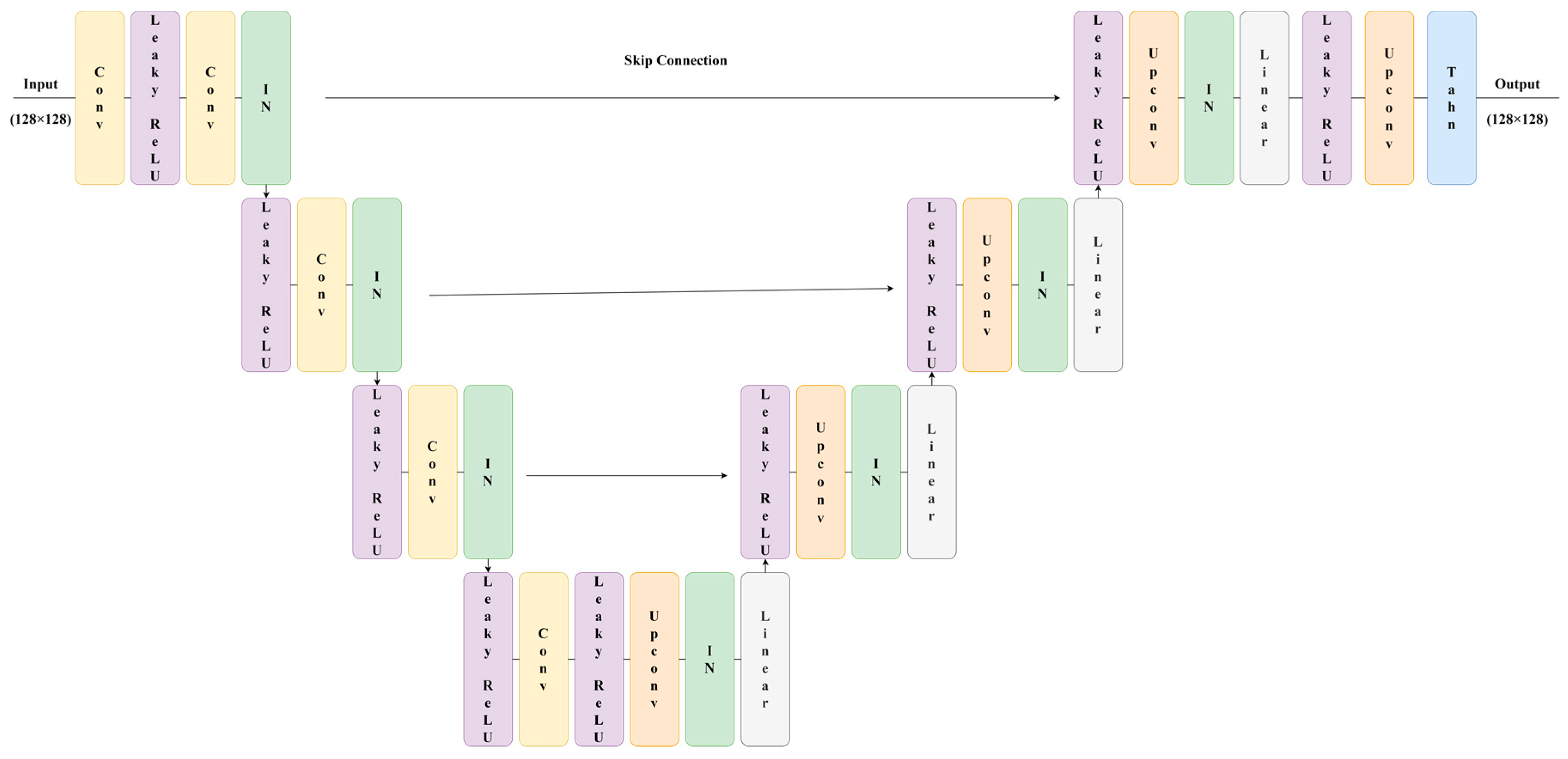
The generator translates an input image into an output image in the target domain and uses Adaptive Instance Normalization (AdaIN) [27] to inject label information into the generator. Then, it generates fake images. The network architecture of the generator is shown in Figure 2.
As is shown in Figure 2, the generator in this study employs the U-net [28] architecture, which includes both up sampling and down sampling. The network undergoes three rounds of up sampling and three rounds of down sampling. The “Upconv” layer represents the up-sample layer that uses a transposed convolution operator. The “Tanh” layer represents the non-linear activation function, Tanh. Additionally, intermediate skip connections enable the network to retain low-level features while performing feature fusion with high-level information. Instance normalization [29] is denoted as “IN”. During up sampling, the IN layer is replaced with the Adaptive Instance Normalization (AdaIN) layer, which consists of the IN and Linear layers. The AdaIN layer incorporates label information through one-hot encoding, thereby allowing the generator to learn the label information of the domain.

2.2.2. Discriminator Network

The discriminator learns to distinguish between real and fake images, whether it is a real image or a fake image generated by the generator, and classifies the real images. The network architecture of the discriminator is shown in Figure 3.
As is shown in Figure 3, the discriminator inputs an image that passes through the convolution layer and finally outputs values. The discriminator adopts the output mode of ACGAN [30] and has two outputs. The first 3*3 convolution output judges the authenticity of the image, with the real image judged as true and the false image is judged as false. The second 1*1 convolution outputs the probability that this picture belongs to two classes, and the maximum class probability is used as the confidence estimation. Furthermore, spectral normalization [31] is added to the discriminator during training to stabilize the training process.

2.2.3. Loss

Adversarial Loss: The adversarial loss is a general loss function of the GAN, which makes the generated image more consistent with the distribution of the target domain, as is shown in Equation (5). The generator G tries to minimize L a d v , and the discriminator D tries to maximize it.
L a d v = E x log D x + E z [ log ( 1 D ( G ( z ) ) ) ]
Domain Classification Loss: For a given input image x and a domain label c , the goal is to translate x into an output image y that is properly classified to the target domain c . To achieve this condition, add an auxiliary classifier on top of D and impose the domain classification loss when optimizing both D and G. The domain classification loss for real images is used to optimize D , as is shown in Equation (6).
L c l s r = E x , c [ log D c l s ( c | x ) ]
The domain classification loss for fake images is used to optimize G , as is shown in Equation (7).
L c l s f = E x , c [ log D c l s ( c | G ( x , c ) ) ]
The term D c l s ( c | x ) represents a probability distribution over domain labels computed by D . By minimizing this objective, D learns to classify a real image x to its corresponding original domain c . Assume that the input image and domain label pair ( x , c ) are given by the training data. G tries to minimize this objective to generate images that can be classified as the target domain c .
Reconstruction Loss: As is shown in Equation (8), G takes as its input the translated image G x , c and the original domain label c , and it tries to reconstruct the original image x . The L1 norm is used as the reconstruction loss.
L r e c = E x , c , c = [ | | x G ( G x , c , c ) | | 1 ]
Identity Loss: When calculating the identity loss of generator G , G inputs y to generate ŷ . Then, use the L1 loss of y and ŷ as the identity loss of G . Correspondingly, the identity loss of generator F is the L1 loss of input x and generated x , as is shown in Equation (9).
L i d e n G , F = E y p d a t a ( y ) [ | | G ( y ) y | | 1 ] + E x p d a t a x [ | | F ( x ) x | | 1 ]
The objective functions to optimize G and D are shown in Equations (10) and (11).
L D = L a d v + λ c l s L c l s r
L G = L a d v + λ c l s L c l s f + λ r e c L r e c + λ i d e n L i d e n
where λ c l s , λ r e c , and λ i d e n are hyper-parameters that control the relative importance of the domain classification, reconstruction loss, and identity loss. λ c l s = 1, λ r e c = 10, and λ i d e n = 1 in the underwater image restoration experiments.

3. Experimental Results

In this section, experiments have been conducted. Section 3.1 comprises the experiments to obtain the improved confidence estimation. Section 3.2 combines the improved confidence estimation method with the built underwater image restoration network to conduct image restoration experiments. Section 3.3 is an experiment that consists of dividing the dataset and then performing multi-domain translation in two stages.

3.1. Confidence Improvement Experiment

In this section, the related issues of training details are described in detail, and then the experimental results are evaluated using different evaluation metrics.

3.1.1. Training Details

In this experiment, PyTorch libraries [32] were used to implement the experiment. The ResNet50 [33] model was trained using SGD, the momentum was 0.55, the initial learning rate was 0.1, the weight decay was 10 5 , and it was trained for 100 epochs. The initial learning rate was set to 0.001 for VGG16 [34] training and ResNet50. The dataset was unpaired from the EUVP dataset [6], 90% of which was used as a training set, and 10% was used as the test set. For data augmentation, the size of the images was adjusted to (128 + 16) × (128 + 16) and then randomly cropped to 128 × 128. When testing, we adjusted the image to (128 + 16) × (128 + 16) and then cropped the center to 128 × 128.

3.1.2. Evaluation Metrics

In [17], to measure ordinal ranking performance, five common metrics were used: the accuracy, the Area Under the Risk–Coverage Curve (AURC) that was defined to be the error rate as a function of coverage, the Excess-AURC (E-AURC) that was a normalized AURC [35], the Area Under the Precision–Recall Curve that used errors as the positive class (AUPR-Error), and the False Positive Rate at 95% True Positive Rate (FPR-95%-TPR). For calibration, we used the Expected Calibration Error (ECE) [36] and the Negative Log Likelihood (NLL).
The improved method proposed in this paper was compared with the method of [17] and the baseline model without the improved method. In this experiment, the baseline model used the ResNet50 network and VGG16 network to do a binary classification task. The dataset used the unpaired files in the EUVP dataset. The loss function used Cross Entropy Loss. Moon’s [17] method added a CRL loss to the baseline, and the method proposed in this paper is based on Moon’s improved method. The obtained comparison results are shown in Table 1 and Table 2.
In Table 1 and Table 2, the AURC and E-AURC values were multiplied by 10 3 , and the NLL was multiplied by 10 for clarity. All remaining values are percentages. The symbol “↑” indicates that higher values are better, and the symbol “↓” indicates that lower values are better. The results in the first row represent the results obtained by the baseline model. The second line is the improvement made by Moon [17] for calculating confidence estimation, and the third line is the improvement proposed in this paper. It can be seen that the accuracy of the improved method is the same as that of Moon’s method, and other indicators had good performance.
In addition, to verify the effect of the proposed method on Deep Ensembles [37], a comparison of experiments was carried out in Table 3. In the training process, all models were trained with SGD with a momentum of 0.9, an initial learning rate of 0.1, and a weight decay of 10 4 . The batch size was 128, and 300 epochs were trained. At 100 epochs and 150 epochs, the learning rate was reduced by a factor of 10. All training results were averaged from experiments using five different random seeds.
The CIFAR-10/100 datasets [38] and the SVHN dataset [39] were exported from the torchvision package of the PyTorch library. For their data augmentation, a random horizontal flip and a 32 × 32 after-filling of 4 pixels per side were used. The standard data augmentation scheme of random cropping was used.
In Table 3, the CIFAR-10 dataset showed improvements in all metrics. Additionally, the SVHN and CIFAR-100 datasets also showed significant improvements in most metrics. Thus, the standard depth model trained with the proposed method improved the quality of confidence estimation and, thus, improved the better performance of the model. However, the improved confidence value estimation algorithm had some limitations, such as a degradation in the performance of the method when for multiple classification tasks.

3.2. Underwater Image Restoration Experiment

In image restoration experiments, it is first necessary to combine the improved confidence estimation algorithm with the image restoration network. Specifically, the improved algorithm is applied to the discriminator of the network, and the class probability of the real image output from the discriminator is continuously optimized to improve the capability of the discriminator.
In the process of image restoration, the training is divided into two stages. The first stage is to add the method of Section 3.1 to the auxiliary classifier of the discriminator to improve the classification performance of the auxiliary classifier. The translation performed in the first stage is the translation of the undivided poor domain and the good domain. After the first stage is completed, the dataset is divided, and the second stage of training is carried out according to the newly divided dataset. A schematic diagram of each stage is shown in Figure 4.
As is shown in Figure 4, the first stage of the training process is the transformation between the distorted domain and the clean domain, and the second stage is the inverse labeling of samples with low confidence values in the clean domain to the distorted domain. Then, both domains are transformed to the domain with high confidence values in the clean domain. For these images, it did not particularly conform to the characteristics of the good domain, and the label needed to be reversed into a distorted domain, so the method in the right figure of Figure 4 was used in the second stage of training. According to the confidence value, domains below 0.55 are considered domains with low confidence values in the clean domain, and inverting their labels as distorted domains can improve the final restoration effect. The label adopted one-hot encoding, and the largest class probability among the two probabilities output by the auxiliary classifier in the discriminator was used as the confidence value. In this section, experiments were performed using Moon’s [17] method and the improved confidence value method combined with image restoration networks, respectively.

3.2.1. Training Details

The dataset used in the experiments and the image restoration process in this section are the same as in Section 3.1. This work uses Adam optimizer [40] with beta1 = 0.5, beta2 = 0.999 and learning rate lr = 0.0001. Additionally, the weight decay value of the discriminator optimizer was 1 × 10⁻⁵.

3.2.2. Evaluation Metrics

We inverted the label value of the sample with a low confidence value, set five random seeds, conducted five experiments, and took the average value. The experimental setup is the same as in Section 3.2. The results are shown in Table 4.
In Table 4, the two average values represent the average metrics of Moon’s method and the method mentioned in this paper after training with five random seeds, respectively. It can be seen that the proposed method was well improved compared to the Moon’s method. Therefore, the next step of the division experiment could be carried out.

3.3. Division Experiment of Underwater Image Restoration

This section builds on Section 3.2, but differs by dividing the training process into two stages. After completion of the first stage, the dataset was divided based on the confidence estimation, and the corresponding index was stored. A threshold was set based on the confidence for division, with a value of 0.55 used in this case, thereby separating higher and lower confidence domains. At the beginning of the second stage, which starts between 50–80 epochs, respectively, the lower confidence domain labels in the good domain were reversed to indicate distorted domains and continued to run through 100 epochs. The test set used the “Inp” file in the “test_sample” folder in EUVP. Table 5 and Table 6 present the comparison results of the experiment’s quantitative and qualitative evaluation.

3.3.1. Quantitative Evaluation

For a quantitative evaluation of the restored images, the UIQM [41] can be used for comparison. UIQM includes three underwater image attribute metrics: Underwater Image Colorimetric Metric (UICM), Underwater Image Sharpness Metric (UISM), and Underwater Image Contrast Metric (UIConM). The higher the UIQM score, the more consistent the results are with human visual perception.
In Table 5, the first row shows the UIQM values obtained from the test set after training using the Section 3.2 method for images without label inversion, which demonstrate an improvement in values. The second and third rows display the UIQM values after label inversion using different epochs. The results show that UIQM values with label inversion performed better than those without inversion, regardless of the epoch. This is because the divided dataset filtered out more blurred images in the clean domain, thereby demonstrating the effectiveness of the proposed method.

3.3.2. Qualitative Evaluation

For the qualitative assessment, the results of the second phase of the test starting from the 80th epoch were chosen to be compared with the results of the unreversed labels, in addition to the DCP method using as a comparison. The results are shown in Table 6.
Table 6 compares the restoration result obtained without dividing the dataset with the restoration result obtained by dividing it into 80s. The traditional method DCP was also used for comparison. The first column shows the original underwater image, and the second column shows the repair result of the low-confidence sample without reversing and low-confidence samples. Although the undivided restoration results improved, the overall appearance was red, while the DCP method produced a dark restoration result. Bycomparison, the division results exhibited a better visual restoration effect. The results show that the proposed method is effective for underwater image restoration, as it achieved good outcomes in both qualitative and quantitative evaluations.

4. Conclusions

This work aimed to improve the visual quality of images by introducing an improved confidence estimation algorithm. The algorithm divides the dataset using the number of consecutive correct predictions during the training period as a confidence estimation, which serves as a real probability ranking to obtain better prediction results. This method improved the classification performance. Moreover, this work built an image restoration network that demonstrated an enhancement in image quality. Finally, the performance of the final image restoration was further improved by applying the improved confidence estimation algorithm to the image restoration network and inverting labels for images with low confidence values in the clean domain as degenerated domain. The experimental results show that the multi-domain transformation method based on domain partitioning is highly effective. Both qualitative and quantitative evaluations confirm improved image restoration quality. It is important to note that the proposed method can preprocess the dataset before network training to enhance the recovery results, and it can be extended to other underwater image restoration networks without the need for additional nodes to output confidence values. Therefore, this method can be added to the algorithms of other authors. However, it does not perform well for extremely blurry images, as is shown in Table 7. Future research will concentrate on restoring blurred images.
Table 7 shows that the network’s recovery of highly blurred images is unsatisfactory and results in further distortion. Therefore, our future work will concentrate on enhancing the processing of such images.

Author Contributions

Conceptualization, methodology, software, validation, investigation, data curation, writing—original draft preparation, T.X.; review and editing, T.X., T.Z. and J.Z. All authors have read and agreed to the published version of the manuscript.

Funding

This research was supported by the Natural Science Foundation of China under Grand (No. 52171310), the National Natural Science Foundation of China (No. 52001039), Research Fund from Science and Technology on Underwater Vehicle Technology Laboratory (No. 2021JCJQ-SYSJJ-LB06903). Shandong Natural Science Foundation in China (No. ZR2019LZH005).

Institutional Review Board Statement

Not applicable.

Informed Consent Statement

Not applicable.

Data Availability Statement

Suggested Data Availability Statements are available at https://irvlab.cs.umn.edu/resources/euvp-dataset (accessed on 10 December 2021).

Acknowledgments

The authors would like to thank the editors and reviewers for their advice.

Conflicts of Interest

The authors declare no conflict of interest.

References

  1. McGlamery, B.L. A computer model for underwater camera systems. Int. Soc. Opt. Photonics 1980, 208, 221–231. [Google Scholar]
  2. Jaffe, J.S. Computer modeling and the design of optimal underwater imaging systems. IEEE J. Ocean. Eng. 1990, 15, 101–111. [Google Scholar] [CrossRef]
  3. Zhou, J.; Wei, X.; Shi, J.; Chu, W.; Lin, Y. Underwater image enhancement via two-level wavelet decomposition maximum brightness color restoration and edge refinement histogram stretching. Opt. Express 2022, 30, 17290–17306. [Google Scholar] [CrossRef] [PubMed]
  4. He, K.; Sun, J.; Tang, X. Single image haze removal using dark channel prior. IEEE Trans. Pattern Anal. Mach. Intell. 2010, 33, 2341–2353. [Google Scholar] [CrossRef] [PubMed]
  5. Liang, Z.; Ding, X.; Wang, Y.; Yan, X.; Fu, X. GUDCP: Generalization of Underwater Dark Channel Prior for Underwater Image Restoration. IEEE Trans. Circuits Syst. Video Technol. 2021, 32, 4879–4884. [Google Scholar] [CrossRef]
  6. Zhou, Y.; Wu, Q.; Yan, K.; Feng, L.; Xiang, W. Underwater image restoration using color-line model. IEEE Trans. Circuits Syst. Video Technol. 2018, 29, 907–911. [Google Scholar] [CrossRef]
  7. Islam, M.J.; Xia, Y.; Sattar, J. Fast underwater image enhancement for improved visual perception. IEEE Robot. Autom. Lett. 2020, 5, 3227–3234. [Google Scholar] [CrossRef] [Green Version]
  8. Chen, L.; Tong, L.; Zhou, F.; Jiang, Z.; Li, Z.; Lv, J.; Dong, J.; Zhou, H. A Benchmark dataset for both underwater image enhancement and underwater object detection. arXiv 2020, arXiv:2006.15789. [Google Scholar] [CrossRef]
  9. Hou, G.; Zhao, X.; Pan, Z.; Yang, H.; Tan, L.; Li, J. Benchmarking underwater image enhancement and restoration, and beyond. IEEE Access 2020, 8, 122078–122091. [Google Scholar] [CrossRef]
  10. WaterGAN: Unsupervised generative network to enable real-time color correction of monocular underwater images. IEEE Robot. Autom. Lett. 2017, 3, 387–394. [CrossRef] [Green Version]
  11. Zhu, J.Y.; Park, T.; Isola, P.; Efros, A.A. Unpaired image-to-image translation using cycle-consistent adversarial networks. In Proceedings of the IEEE International Conference on Computer Vision, Venice, Italy, 22–29 October 2017; pp. 2223–2232. [Google Scholar] [CrossRef]
  12. Fabbri, C.; Islam, M.J.; Sattar, J. Enhancing underwater imagery using generative adversarial networks. In Proceedings of the 2018 IEEE International Conference on Robotics and Automation (ICRA), Brisbane, Australia, 21–25 May 2018; IEEE: Piscataway, NJ, USA, 2018; pp. 7159–7165. [Google Scholar] [CrossRef] [Green Version]
  13. Islam, M.J.; Luo, P.; Sattar, J. Simultaneous enhancement and super-resolution of underwater imagery for improved visual perception. arXiv 2020, arXiv:2002.01155. [Google Scholar] [CrossRef]
  14. Li, C.; Guo, C.; Ren, W.; Cong, R.; Hou, J.; Kwong, S.; Tao, D. An underwater image enhancement benchmark dataset and beyond. IEEE Trans. Image Process. 2019, 29, 4376–4389. [Google Scholar] [CrossRef] [PubMed] [Green Version]
  15. Hong, L.; Wang, X.; Xiao, Z.; Zhang, G.; Liu, J. WSUIE: Weakly supervised underwater image enhancement for improved visual perception. IEEE Robot. Autom. Lett. 2021, 6, 8237–8244. [Google Scholar] [CrossRef]
  16. Deng, J.; Dong, W.; Socher, R.; Li, L.-J.; Li, K.; Fei-Fei, L. Imagenet: A large-scale hierarchical image database. In Proceedings of the 2009 IEEE Conference on Computer Vision and Pattern Recognition, Miami, FL, USA, 20–25 June 2009; IEEE: Piscataway, NJ, USA, 2009; pp. 248–255. [Google Scholar] [CrossRef] [Green Version]
  17. Moon, J.; Kim, J.; Shin, Y.; Hwang, S. Confidence-aware learning for deep neural networks. In Proceedings of the International Conference on Machine Learning, PMLR, Virtual, 13–18 July 2020; pp. 7034–7044. [Google Scholar] [CrossRef]
  18. Goodfellow, I.; Pouget-Abadie, J.; Mirza, M.; Xu, B.; Warde-Farley, D.; Ozair, S.; Courville, A.; Bengio, Y. Generative adversarial networks. Commun. ACM 2020, 63, 139–144. [Google Scholar] [CrossRef]
  19. Isola, P.; Zhu, J.Y.; Zhou, T.; Efros, A.A. Image-to-image translation with conditional adversarial networks. In Proceedings of the IEEE Conference on Computer Vision and Pattern Recognition, Honolulu, HI, USA, 21–26 July 2017; pp. 1125–1134. [Google Scholar] [CrossRef]
  20. Li, C.; Guo, J.; Guo, C. Emerging from water: Underwater image color correction based on weakly supervised color transfer. IEEE Signal Process. Lett. 2018, 25, 323–327. [Google Scholar] [CrossRef] [Green Version]
  21. Liu, P.; Wang, G.; Qi, H.; Zhang, C.; Zheng, H.; Yu, Z. Underwater image enhancement with a deep residual framework. IEEE Access 2019, 7, 94614–94629. [Google Scholar] [CrossRef]
  22. Park, J.; Han, D.K.; Ko, H. Adaptive weighted multi-discriminator CycleGAN for underwater image enhancement. J. Mar. Sci. Eng. 2019, 7, 200. [Google Scholar] [CrossRef] [Green Version]
  23. Maniyath, S.R.; Vijayakumar, K.; Singh, L.; Sharma, S.K.; Olabiyisi, T. Learning-based approach to underwater image dehazing using CycleGAN. Arab. J. Geosci. 2021, 14, 1908. [Google Scholar] [CrossRef]
  24. Wang, P.; Chen, H.; Xu, W.; Jin, S. Underwater image restoration based on the perceptually optimized generative adversarial network. J. Electron. Imaging 2020, 29, 033020. [Google Scholar] [CrossRef]
  25. Zhai, L.; Wang, Y.; Cui, S.; Zhou, Y. Enhancing Underwater Image Using Degradation Adaptive Adversarial Network. In Proceedings of the 2022 IEEE International Conference on Image Processing (ICIP), Bordeaux, France, 16–19 October 2022; IEEE: Piscataway, NJ, USA, 2022; pp. 4093–4097. [Google Scholar] [CrossRef]
  26. Choi, Y.; Choi, M.; Kim, M.; Ha, J.W.; Kim, S.; Choo, J. Stargan: Unified generative adversarial networks for multi-domain image-to-image translation. In Proceedings of the IEEE Conference on Computer Vision and Pattern Recognition, Salt Lake City, UT, USA, 18–22 June 2018; pp. 8789–8797. [Google Scholar] [CrossRef]
  27. Huang, X.; Belongie, S. Arbitrary style transfer in real-time with adaptive instance normalization. In Proceedings of the IEEE International Conference on Computer Vision, Venice, Italy, 22–29 October 2017; pp. 1501–1510. [Google Scholar] [CrossRef]
  28. Ronneberger, O.; Fischer, P.; Brox, T. U-net: Convolutional networks for biomedical image segmentation. In Proceedings of the Conference on Medical image Computing and Computer-Assisted Intervention, Munich, Germany, 5–9 October 2015; Springer: Cham, Switzerland, 2015; pp. 234–241. [Google Scholar] [CrossRef] [Green Version]
  29. Ulyanov, D.; Vedaldi, A.; Lempitsky, V. Instance normalization: The missing ingredient for fast stylization. arXiv 2016, arXiv:1607.08022. [Google Scholar] [CrossRef]
  30. Odena, A.; Olah, C.; Shlens, J. Conditional image synthesis with auxiliary classifier gans. In Proceedings of the International Conference on Machine Learning, PMLR, Sydney, Australia, 6–11 August 2017; pp. 2642–2651. [Google Scholar] [CrossRef]
  31. Miyato, T.; Kataoka, T.; Koyama, M.; Yoshida, Y. Spectral normalization for generative adversarial networks. arXiv 2018, arXiv:1802.05957. [Google Scholar] [CrossRef]
  32. Paszke, A.; Gross, S.; Massa, F.; Lerer, A.; Bradbury, J.; Chanan, G.; Killeen, T.; Lin, Z.; Gimelshein, N.; Antiga, L.; et al. Pytorch: An imperative style, high-performance deep learning library. Adv. Neural Inf. Process. Syst. 2019, 32. [Google Scholar] [CrossRef]
  33. He, K.; Zhang, X.; Ren, S.; Sun, J. Deep residual learning for image recognition. In Proceedings of the IEEE Conference on Computer Vision and Pattern Recognition, Las Vegas, NV, USA, 27–30 June 2016; pp. 770–778. [Google Scholar] [CrossRef] [Green Version]
  34. Simonyan, K.; Zisserman, A. Very deep convolutional networks for large-scale image recognition. arXiv 2014, arXiv:1409.1556. [Google Scholar] [CrossRef]
  35. Geifman, Y.; Uziel, G.; El-Yaniv, R. Bias-reduced uncertainty estimation for deep neural classifiers. In Proceedings of the International Conference on Learning Representations, New Orleans, LA, USA, 6–9 May 2019. [Google Scholar] [CrossRef]
  36. Naeini, M.P.; Cooper, G.; Hauskrecht, M. Obtaining well calibrated probabilities using bayesian binning. In Proceedings of the Twenty-Ninth AAAI Conference on Artificial Intelligence, Austin, TX, USA, 25–30 January 2015. [Google Scholar] [CrossRef]
  37. Lakshminarayanan, B.; Pritzel, A.; Blundell, C. Simple and scalable predictive uncertainty estimation using deep ensembles. Adv. Neural Inf. Process. Syst. 2017, 30, 6402–6413. [Google Scholar] [CrossRef]
  38. Krizhevsky, A.; Hinton, G. Learning Multiple Layers of Features from Tiny Images; Technical Report TR-2009; University of Toronto: Toronto, ON, Canada, 2009. [Google Scholar]
  39. Netzer, Y.; Wang, T.; Coates, A.; Bissacco, A.; Wu, B.; Ng, A.Y. Reading Digits in Natural Images with Unsupervised Feature Learning. In Proceedings of the NIPS Workshop on Deep Learning and Unsupervised Feature Learning, Granada, Spain, 12–17 December 2011; Available online: https://storage.googleapis.com/pub-tools-public-publication-data/pdf/37648.pdf (accessed on 5 January 2023).
  40. Kingma, D.P.; Ba, J. Adam: A method for stochastic optimization. arXiv 2014, arXiv:1412.6980. [Google Scholar] [CrossRef]
  41. Panetta, K.; Gao, C.; Agaian, S. Human-visual-system-inspired underwater image quality measures. IEEE J. Ocean. Eng. 2015, 41, 541–551. [Google Scholar] [CrossRef]
Figure 1. Examples of the underwater synthetic dataset EUVP [7]. (a,b): distorted image. (c,d): clean image.
Jmse 11 00674 g001
Figure 2. The architecture of the generator.
Jmse 11 00674 g002
Figure 3. The architecture of the discriminator.
Jmse 11 00674 g003
Figure 4. Overview of domain translation.
Jmse 11 00674 g004
Table 1. Comparison of ResNet50.
MethodAccuracy
(↑)
AURC
(↓)
EAURC
(↓)
AUPR
(↑)
FPR
(↓)
ECE
(↓)
NLL
(↓)
Brier
(↓)
Baseline [17]93.829.177.2244.1141.14.773.4310.67
Moon [17]94.066.14.346.3739.061.21.848.83
Proposed94.065.844.0347.4338.720.961.88.77
Table 2. Comparison of VGG16.
MethodAccuracy
(↑)
AURC
(↓)
EAURC
(↓)
AUPR
(↑)
FPR
(↓)
ECE
(↓)
NLL
(↓)
Brier
(↓)
Baseline [17]98.581.671.6726.733.331.240.962.53
Moon [17]97.951.41.1936.5923.081.480.763.32
Proposed98.580.910.8121.122.221.090.562.66
Table 3. Experimental results based on DenseNet-121 network.
Model
Dataset
MethodAccuracy
(↑)
AURC
(↓)
EAURC
(↓)
AUPR
(↑)
FPR
(↓)
ECE
(↓)
NLL
(↓)
Brier
(↓)
DenseNet-121
CIFAR-10
Baseline [17]88.76 ± 0.4420.21 ± 2.1213.61 ± 0.4649.08 ± 2.4156.58 ± 2.397.86 ± 0.195.71 ± 0.0918.81 ± 1.04
Moon [17]89.17 ± 0.1918.62 ± 2.412.52 ± 1.2449.13 ± 2.3854.57 ± 5.103.21 ± 0.093.59 ± 0.0316.15 ± 0.48
Proposed89.22 ± 0.118.25 ± 0.8512.22 ± 0.3449.96 ± 0.8253.39 ± 2.482.99 ± 0.043.54 ± 0.0115.99 ± 0.21
DenseNet-121
CIFAR-100
Baseline [17]60.49 ± 0.79158.38 ± 54.4267.33 ± 8.8774.51 ± 0.3767.46 ± 0.3518.59 ± 0.1318.67 ± 0.2357.23 ± 1.22
Moon [17]62.63 ± 0.34141.51 ± 15.4160.87 ± 1.6274.29 ± 0.5665.78 ± 3.2514.36 ± 0.0215.95 ± 0.0852.39 ± 0.6
Proposed62.6 ± 0.52140.53 ± 18.3459.75 ± 2.2974.43 ± 0.3266.21 ± 0.7714.54 ± 0.3315.85 ± 0.152.32 ± 0.82
DenseNet-121
SVHN
Baseline [17]95.45 ± 0.038.85 ± 2.57.8 ± 2.540.47 ± 5.1337.54 ± 6.73 ± 0.022.45 ± 0.017.7 ± 0.08
Moon [17]95.83 ± 0.015.53 ± 0.044.65 ± 0.0545.07 ± 4.1431.91 ± 4.640.65 ± 0.0031.64 ± 0.0016.43 ± 0.02
Proposed95.99 ± 0.035.29 ± 0.024.47 ± 0.0243.87 ± 3.7631.29 ± 3.640.63 ± 0.0011.59 ± 0.0036.20 ± 0.04
Table 4. Comparison between the improved method and the original method in the underwater image restoration network.
ModelRandom
Seed
AccuracyAURCEAURCAUPRFPRECENLLBrier
Moon [17]10094.497.425.8733.7148.572.611.698.66
10194.337.856.2132.6361.113.031.849.13
10294.968.166.8737.940.622.471.767.64
10394.027.795.9739.09503.281.849.21
10491.3415.211.3451.1450.914.762.812.44
Average
Value
93.839.287.2538.8950.243.231.999.42
93.768.376.2639.8246.583.381.799.24
Proposed10096.064.53.7227.57482.321.26.67
10194.4910.328.7738.4251.432.81.888.73
10292.287.924.875730.614.561.910.01
10394.177.65.8733.643.242.841.78.68
10491.8111.58.0542.5259.624.372.2712.11
Table 5. The UIQM value comparison of a different epoch.
Input UIQM
2.57 ± 0.55
Not Inversion3.22 ± 0.33
Label Inversed 50th60th70th80th
3.24 ± 0.343.24 ± 0.323.24 ± 0.313.26 ± 0.4
Table 6. Qualitative comparison of the underwater images.
Original ImageNot ReverseDCP80th
Jmse 11 00674 i001Jmse 11 00674 i002Jmse 11 00674 i003Jmse 11 00674 i004
Jmse 11 00674 i005Jmse 11 00674 i006Jmse 11 00674 i007Jmse 11 00674 i008
Jmse 11 00674 i009Jmse 11 00674 i010Jmse 11 00674 i011Jmse 11 00674 i012
Jmse 11 00674 i013Jmse 11 00674 i014Jmse 11 00674 i015Jmse 11 00674 i016
Jmse 11 00674 i017Jmse 11 00674 i018Jmse 11 00674 i019Jmse 11 00674 i020
Table 7. Badly translated images.
Original imageJmse 11 00674 i021Jmse 11 00674 i022Jmse 11 00674 i023
Restored imageJmse 11 00674 i024Jmse 11 00674 i025Jmse 11 00674 i026
Disclaimer/Publisher’s Note: The statements, opinions and data contained in all publications are solely those of the individual author(s) and contributor(s) and not of MDPI and/or the editor(s). MDPI and/or the editor(s) disclaim responsibility for any injury to people or property resulting from any ideas, methods, instructions or products referred to in the content.