Course-Keeping Performance of a Container Ship with Various Draft and Trim Conditions under Wind Disturbance

Abstract

IMO presented the standard for ship’s manoeuvrability which every ship is recommended to satisfy. Although it specifies a full load and even keel condition as the condition at which the standard applies, practically, ships are operated under various loading conditions of cargo. From this viewpoint, the authors have conducted manoeuvring tests of a container ship under five loading conditions with different combinations of the draft and trim, and one of the authors established the manoeuvring mathematical model of the ship for each condition so far. This study focuses on the course-keeping performance of the same ship under these loading conditions under wind disturbance. It is the aim of this study to discuss both the influences of loading condition and wind condition simultaneously on the check helm and attitude of the ship while maintaining the target course. For this purpose, the arrangement of containers and their weight distribution were designed as exact as possible. For example, the ship with a trim by bow, which is commonly preferred for fuel efficiency, needs to have a larger check helm for course keeping, especially under the condition of wind disturbance diagonally from behind. This kind of knowledge would be useful for safe navigation.

1. Introduction

The IMO presents a standard for ship manoeuvrability which every ship is recommended to satisfy for navigation safety [1]. Although it specifies a full load and even keel condition as the conditions at which the standard applies, ships are operated under various loading conditions of cargoes in daily navigation. In particular, in the case of a container ship, the number of cargoes is influenced by the shipping market, affecting the displacement or daft of the ship. In addition, trim, which is an important factor in improving fuel efficiency, has been an interesting concern in recent years (e.g., [2,3]). Although such a loading condition or ship’s attitude, that is, draft and trim, is likely to affect the navigation performance, there have been few studies on its effect on manoeuvrability compared to those on the resistance and propulsive performances. From this viewpoint, the authors have conducted free-manoeuvring experiments for a container ship with five different loading conditions, such as even keel/full loaded condition, shallow draft/light loaded condition, and deep draft/overloaded condition, in addition to trim by stern condition and trim by bow condition [4]. CFD analysis was also applied to explain the trim and draft effects on hydrodynamic force characteristics. Furthermore, one of the authors continuously established a manoeuvring mathematical model of the subject ship based on captive model experiments [5].

In general, the effect of wind on a ship’s motion characteristics is significant. For ex-ample, Zhou et al. [6] quantitatively analysed and estimated the impacts of external conditions (wind and current) on ship behaviour in ports and waterways based on AIS data. Regarding studies on ships’ motion under wind, Yoshimura and Nagashima [7] discussed the manoeuvring motion of a PCC through the free-running model test and simulation in uniform wind. Hasegawa et al. [8] discussed the comparison of the course-keeping ability of a PCC when installing a normal rudder and high-lift rudder in windy conditions. Nagarajan et al. [9] developed the mathematical model of a VLCC and carried out full-scale course-keeping simulations under gusting wind conditions. Paroka et al. [10] also ran the simulation to discuss the wind effect on the ship manoeuvrability of an Indonesian ro-ro ferry in steady wind. Im and Tran [11] estimated the equilibrium state of a behaviour of a training ship under the influence of wind. Some other numerical studies have also been performed so far (e.g., [12,13]). Since a container ship has a large windage area due to the large number of containers on the deck, it has been also a major research target. Andersen [14] investigated a post-Panamax container ship through a series of wind tunnel tests. Janssen [15] presented RANS CFD simulations of wind loads on a container ship and validated with Andersen [14]. Seok and Park [16] also numerically studied the effect of the presence of the superstructure on the resistance, trim, and sinkage of an 8000 TEU-class container ship.

As seen from those references, although there have been many studies so far, most studies have only focused on one loading condition, and no studies have discussed the effect of the combination of the loading condition (or ship’s attitude) and wind on the manoeuvring performance. Because the authors found that the change of course stability was highly sensitive to the loading conditions [4], it is interesting to the change the course-keeping performance, which is the most fundamental factor for navigation safety, by considering both hydrodynamic force acting on the hull under water and aerodynamic force on the hull/containers above water simultaneously. In this study, the superstructure and container arrangement of the subject container ship were designed for five different loading conditions, and the wind force and moment acting on the ship were estimated using an authorized empirical formula. Subsequently, the difference in the course-keeping performance of the ship under different loading conditions and under various wind conditions was investigated.

The structure of this article is as follows. Section 2 through 5 outline the methodology. The subject ship is described in Section 2, and the manoeuvring mathematical model, including the motion equations and the formulations of forces and moments acting on the ship, are explained in Section 3. The over-deck objects are designed and wind forces are estimated in Section 4. The mathematical model is validated in Section 5. The results and discussions for the course-keeping performance under wind are presented in Section 6 (dynamic simulation) and Section 7 (equilibrium state). Finally, Section 8 provides the conclusions.

2. Subject Ship (KCS Container Ship)

2.1. Principal Dimensions

The subject ship in this study is the container ship KCS [17], which has been developed for research purposes. Many studies have been conducted using this ship (e.g., [18,19]), and the authors’ previous studies [4,5] have also used it as well.

Table 1. Length and breadth of the subject ship.

Item	Symbol	Real Scale	Model Scale
Length	$L$ [m]	230	3.057
Breadth	B [m]	32.2	0.428

lists the length and breadth of this ship. Other principal dimensions, such as the draft and displacement, are explained in the following section.

Table 2. Principal dimensions of the propeller and rudder of the subject ship.

Item		Symbol	Real Scale	Model Scale
Propeller	Diameter	$D_P$ [m]	7.9	0.105
	Pitch ratio	P/$D_P$	0.997	0.997
Rudder	Height	$H_R$ [m]	9.9	0.132
	Cord length	$B_R$ [m]	5.5	0.0731
	Aspect ratio	$\Lambda$	1.8	1.8
	Area w/ horn	$A_R$ [m2]	54.43	0.0096

lists the principal dimensions of the propeller and the rudder. Notably, the hydrodynamic force data, measured in the towing tank experiment using a 1/75.24-scale model [5], were used for the simulation. Therefore, the model- and real-scale dimensions are listed in these tables.

This ship has a 230 (m) full-scale length between perpendiculars and can load 3600 TEU (twenty-foot equivalent unit) containers. Because this type of container ship is handy and can avoid getting caught in the depth restriction of most harbours, many ships have been in service and may continue to be one of the standard container ship sizes in the future.

2.2. Loading Conditions

Five loading conditions were set for the subject ship in this study. Hereafter, they are named after their drafts and trims. EK, which represents the full-load draft and even keel, is the standard among the considered conditions. S-EK has a shallow draft with an even keel, which assumes that a small number of containers are loaded on the ship. D-EK has a deep draft and an even keel and was designed to be slightly heavier than EK. Such an overload condition was also set up to investigate the risk of reduced manoeuvrability when the load condition was overweighed. Meanwhile, in terms of the trim series, TS represents the trim by the stern, and TB represents the trim by the bow. They have the same draft at the midship as EK. The loading conditions are presented in

Table 3. Loading conditions, i.e., drafts, displacement, block coef., of the subject ship.

Symbol	S-EK	TS	EK	TB	D-EK
$d_a$ [m]	9.6	11.99	10.8	9.6	11.99
$d_m$ [m]	9.6	10.8	10.8	10.8	11.99
$d_f$ [m]	9.6	9.6	10.8	11.99	11.99
$\nabla$ [m3]	44,889	52,044	52,044	52,044	59,625
$C_b$	0.631	0.651	0.651	0.651	0.671

, where $d_a$, $d_m$, and $d_f$ represent the draft at the AP, midship, and FP; and $\nabla$ and $C_b$ represent the displacement and block coefficient, respectively. The position of the centre of gravity and the radius of gyration are described in the following section.

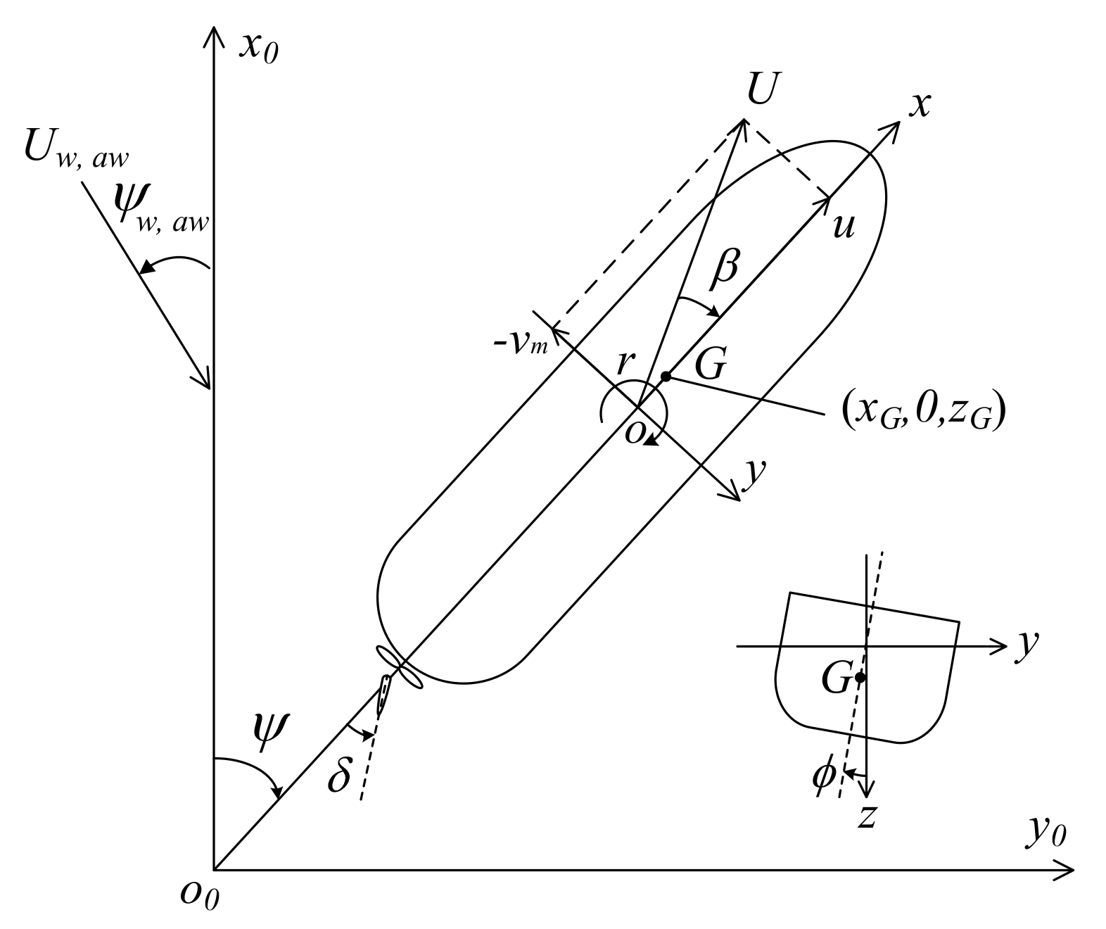
2.3. Coordinate Systems

Four degrees-of-freedom motions: surge, sway, yaw, and roll motions, were considered. They are based on the right-hand coordinate system shown in Figure 1. The space-fixed coordinate system $o_0$-$x_0{y}_0{z}_0$ was considered with the plane referring to the still water surface. The heading angle of the ship $\psi$, true wind angle ${\psi }_w$, and apparent wind angle ${\psi }_{aw}$ were defined as the angles from the $x_0$ axis. In addition, the horizontal body axis coordinate system [20], that is, $o$-$xyz$, was considered, where the origin was set at the midship, and the $x$- and $y$-axes were on the bow and starboard sides, respectively. The $z$ axis was vertically directed downward. The roll angle $\varphi$ takes positive when the ship was inclined to the right. $G$ represents the position of the centre of gravity (C.G.) of the ship, and its position is expressed as ($x_G$, 0, $z_G$). $u$ and $v_m$ are the surge and sway velocities at the midship, respectively, which are used to calculate ship speed $U$ and hull drift angle $\beta$. $U_w$ and $U_{aw}$ are the true and apparent wind velocities, respectively. Furthermore, $r$ is the yaw rate, and the rudder angle is denoted as $\delta$.

3. Manoeuvring Mathematical Model

The manoeuvring mathematical model of this container ship was established in [5], which included one of the authors of this study. It is based on the MMG model which is a standard ship manoeuvring model [21].

3.1. Motion Equations

Motion equations with four degrees of freedom were defined as follows: These are ordinary differential equations based on a ship-fixed coordinate system.

$$\begin{array}{l}\left(m+m_x\right)\dot{u}-\left(m+m_y\right)v_{m}r-m{x}_G{r}^2+m{z}_{G}r\dot{\varphi }=X\\ \left(m+m_y\right){\dot{v}}_m+\left(m+m_x\right)ur+m{x}_G\dot{r}-\left(m_y{\alpha }_z+m{z}_G\right)\ddot{\varphi }=Y\\ \left(I_{zz}+J_{zz}+m{x}_G^2\right)\dot{r}+m{x}_G\left({\dot{v}}_m-z_G\ddot{\varphi }+ur\right)=N\\ \left(I_{xx}+J_{xx}+m{z}_G^2\right)\ddot{\varphi }-\left(m_y {\alpha }_z+m{z}_G\right){\dot{v}}_m-m{z}_G \left(x_G\dot{r}+ur\right)=K\end{array}\}$$

(1)

where the time derivative is distinguished by placing a dot above the variable. $m$ is the mass of the ship. $m_x$ and $m_y$ are the added messes in surge and sway. $I_{zz}$ is the moment of inertia, $J_{zz}$ is the added moment of inertia with respect to the yaw motion, while $I_{xx}$ and $J_{xx}$ are those moments of inertia with respect to the roll motion. ${\alpha }_z$ is the vertical acting point of the added mass in sway. On the right-hand side, $X$ and $Y$ are the hydrodynamic surge and sway forces acting on the ship without the added mass components. $N$ and $K$ are the hydrodynamic yaw and roll moments without the added moments of the inertial components, respectively.

3.2. Formulation of Hydrodynamic Forces and Moments

The hydrodynamic forces and moments acting on the ship were formulated as follows.

$$\begin{array}{l}X=X_H+X_P+X_R+X_A\\ Y=Y_H+Y_R+Y_A\\ N=N_H+N_R+N_A\\ K=-Y_H z_H-Y_R z_R-mg\overline{GM}\varphi +K_{\dot{\varphi }}\dot{\varphi }+K_{\dot{\varphi }\dot{\varphi }}\dot{\varphi }\left|\dot{\varphi }\right|+K_A\end{array}\}$$

(2)

where the subscripts H, P, R, and A signify the hull, propeller, rudder, and wind, respectively. In terms of the roll moment, the first and second terms represent the roll moment owing to the hull sway force and ruder normal force where $z_H$ and $z_R$ are the vertical acting points of them from G. The roll restoring moment is considered as the third term, where $\overline{GM}$ is the distance between the centre of gravity and the metacentre, and $g$ is the gravitational acceleration. The roll damping moment is expressed by the sum of the fourth and fifth terms where $K_{\dot{\varphi }}$ and $K_{\dot{\varphi }\dot{\varphi }}$ are the roll damping coefficients.

3.2.1. Hull Force

The hydrodynamic forces and moment on the hull are formulated as follows.

$$\begin{array}{l}{X}_H=1/2\rho L{d}_m{U}^2{X}_H^{\prime }\\ Y_H=1/2\rho L{d}_m{U}^2{Y}_H^{\prime }\\ N_H=1/2 \rho L{d}_m U^2{N}_H^{\prime }\end{array}\}$$

(3)

where

$$\begin{array}{l}{X}_H^{\prime }=-R_0^{\prime }+X_{vv}^{\prime }{v_m^{\prime }}^2+X_{vr}^{\prime }{v}_m^{\prime }{r}^{\prime }+X_{rr}^{\prime }{r^{\prime }}^2+X_{vvvv}^{\prime }{v_m^{\prime }}^4+X_{v\varphi }^{\prime }{v}_m^{\prime }\varphi +X_{r\varphi }^{\prime }{r}^{\prime }\varphi +X_{\varphi \varphi }^{\prime }{\varphi }^2\\ Y_H^{\prime }=Y_v^{\prime }{v}_m^{\prime }+Y_r^{\prime }{r}^{\prime }+Y_{vvv}^{\prime }{v_m^{\prime }}^3+Y_{vvr}^{\prime }{v_m^{\prime }}^2{r}^{\prime }+Y_{vrr}^{\prime }{v}_m^{\prime }{r^{\prime }}^2+Y_{rrr}^{\prime }{r^{\prime }}^3\\ +Y_{\varphi }^{\prime }\varphi +Y_{vv\varphi }^{\prime }{v_m^{\prime }}^2\varphi +Y_{rr\varphi }^{\prime }{r^{\prime }}^2\varphi +Y_{v\varphi \varphi }^{\prime }{v}_m^{\prime }{\varphi }^2+Y_{r\varphi \varphi }^{\prime }{r}^{\prime }{\varphi }^2\\ N_H^{\prime }=N_v^{\prime }{v}_m^{\prime }+N_r^{\prime }{r}^{\prime }+N_{vvv}^{\prime }{v_m^{\prime }}^3+N_{vvr}^{\prime }{v_m^{\prime }}^2{r}^{\prime }+N_{vrr}^{\prime }{v}_m{r^{\prime }}^2+N_{rrr}^{\prime }{r^{\prime }}^3\\ +N_{\varphi }^{\prime }\varphi +N_{vv\varphi }{v_m^{\prime }}^2 \varphi +N_{rr\varphi }^{\prime }{r^{\prime }}^2\varphi +N_{v\varphi \varphi }^{\prime }{v}_m^{\prime }{\varphi }^2+N_{r\varphi \varphi }^{\prime }{r}^{\prime }{\varphi }^2\end{array}\}$$

(4)

where the prime sign signifies non-dimensionality. $\rho$ is the water density. $R_0^{\prime }$ is the resistance coefficient when running straight. The hydrodynamic force derivatives, for example, $X_{vr}^{\prime }$, $X_{v\varphi }^{\prime }$, $Y_v^{\prime }$, $Y_{vvr}^{\prime }$, $N_r^{\prime }$, $N_{r\varphi \varphi }^{\prime }$, represent the magnitude of the force and moment due to manoeuvring motions, such as sway, yaw, and roll, or these coupled motions.

3.2.2. Propeller Force

The propeller force was calculated using the thrust with the thrust deduction factor $t_P$.

$$X_P=\left(1-t_P\right)\rho n_P^2{D}_P^4{K}_T$$

(5)

where

$$K_T=K_0+K_1{J}_P+K_2{J}_P{}^2$$

(6)

where $K_{0,1,2}$ are the coefficients of the propeller thrust open-water characteristic, $K_T$. The number of propeller rotations is denoted as $n_P$, and the propeller advance ratio, $J_P$, is expressed as follows:

$$J_P=u\left(1-w_P\right)/\left(n_P{D}_P\right)$$

(7)

where $w_P$ is the wake coefficient at the propeller position, and it is assumed to change according to the manoeuvring motions, as follows:

$$w_P=\left(w_{P0}-w_{Pmin}\right)\exp \left(-C_0{\beta }_P^2\right)+w_{Pmin}$$

(8)

where $w_{P0}$ is the effective wake fraction during the straight running. $C_0$ and $w_{Pmin}$ are the coefficients representing the wake behaviour against ${\beta }_P$, which is the geometrical inflow angle to the propeller during manoeuvring. This is defined as follows.

$${\beta }_P=\beta -x_P^{\prime }{r}^{\prime }+z_P^{\prime }{\dot{\varphi }}^{\prime }$$

(9)

where $x_P$ and $z_P$ are the longitudinal and vertical coordinates, respectively, of the propeller positions.

3.2.3. Rudder Force

The rudder force was formulated as follows.

$$\left.\begin{array}{c}{X}_R=-\left(1-t_R\right)F_N\sin \delta \cos \varphi \\ Y_R=-\left(1+a_H\right)F_N\cos \delta \cos \varphi \\ N_R=-\left(x_R+a_H{x}_H\right)F_N\cos \delta \cos \varphi \end{array} \right\}$$

(10)

where $t_R$, $a_H$, and $x_H$ denote the rudder–hull interaction factors. The rudder normal force $F_N$ was formulated as follows.

$$F_N=1/2\rho A_R{f}_{\alpha }\left(u_R^2+v_R^2\right)\sin \left\{\delta -ta{n}^{-1}\left(\frac{u_R}{v_R}\right)\right\}$$

(11)

where $f_{\alpha }$ denotes the gradient of the lift coefficient of the rudder. $u_R$ is the propeller-accelerated axial inflow velocity at the rudder and is expressed as follows:

$$u_R=\epsilon u\left(1-w_P\right)\sqrt{\frac{D_P}{H_R}{\left\{1+\frac{k_x}{\epsilon }\left(\sqrt{1+\frac{8K_T}{\pi J_P^2}}-1\right)\right\}}^2+\left(1-\frac{D_P}{H_R}\right)}$$

(12)

where $k_x$ is the flow acceleration rate due to the propeller and $\epsilon$ is the wake fraction ratio at the propeller and rudder positions. The lateral inflow velocity at the rudder, $v_R$, is expressed as follows by considering the flow straightening coefficient, ${\gamma }_R$, which reduces the geometrical inflow angle during manoeuvring:

$$v_R=U{\gamma }_R\left(\beta -l_R^{\prime }{r}^{\prime }+z_R^{\prime }{\dot{\varphi }}^{\prime }\right)$$

(13)

The term in the blanket represents the effective inflow angle at the rudder, where $l_R^{\prime }$ is the effective longitudinal coordinate of the rudder position.

3.2.4. Wind Force

Fujiwara et al. [22] proposed a method to estimate the longitudinal and lateral wind forces and yaw and roll moments for various ships based on the form-related parameters of the ship. It was developed through regression analysis using various wind tunnel experimental data from many wind tunnels. In their reference, the validation was conducted by comparing the estimated value with those of other methods, and the authors proved that the standard error against the experimental data was smaller than that of the others. It is considered a practical method of estimating the wind forces and moments. Its use is recommended by the ITTC [23] in the case of an unavailability of wind tunnel measurements. For example, the lateral wind force, $Y_A$, was calculated by the following equation, where the first term on the right-hand side expresses the lateral component of the cross-flow drag, and the second term expresses that of the lift and induced drag.

$$Y_A=\frac{1}{2}{\rho }_a{U}_{aw}^2{A}_L\left\{C_{CF}{\sin }^2{\psi }_{aw}+C_{YLI}\left(\cos {\psi }_{aw}+\frac{1}{2}{\sin }^2{\psi }_{aw}\cos {\psi }_{aw}\right)\frac{1}{2}\sin 2{\psi }_{aw}\right\}$$

(14)

where

$$C_{CF}={\alpha }_0+{\alpha }_1\frac{A_F}{B{H}_{BR}}+{\alpha }_2\frac{H_{BR}}{L_{OA}}$$

(15)

$$C_{YLI}=\pi \frac{A_L}{L_{OA}^2}+\left\{\begin{array}{c}{\gamma }_{10}+{\gamma }_{11}\frac{A_F}{L_{OA}B} \left(0^{°}\le {\psi }_{aw}\le {90}^{°}\right)\\ {\gamma }_{20}+{\gamma }_{21}\frac{A_{OD}}{L_{OA}^2} \left({90}^{°}\le {\psi }_{aw}\le {180}^{°}\right)\end{array}\right.$$

(16)

where ${\rho }_a$ is the air density. Some parameters related to the windage area were used, that is, $A_F$: projected frontal area above waterline, $A_L$: projected lateral area above waterline, $H_{BR}$: height to top of superstructure, $A_{OD}$: lateral projected area of superstructure and containers on the deck, $L_{OA}$: ship length overall, and ${\mathsf{\alpha }}_i$ and ${\mathsf{\gamma }}_{ij}$ where $i$, $j$ take 0, 1, or 2: regression parameters.

4. Estimation of Wind Forces Acting on the Ship

The hydrodynamic water forces acting on the KCS were measured through towing tank tests, and all experimental coefficients have already been identified [5]. Because the ship model used in the experiment had no objects on the deck, it was necessary to design the superstructure and arrange the containers according to each loading condition.

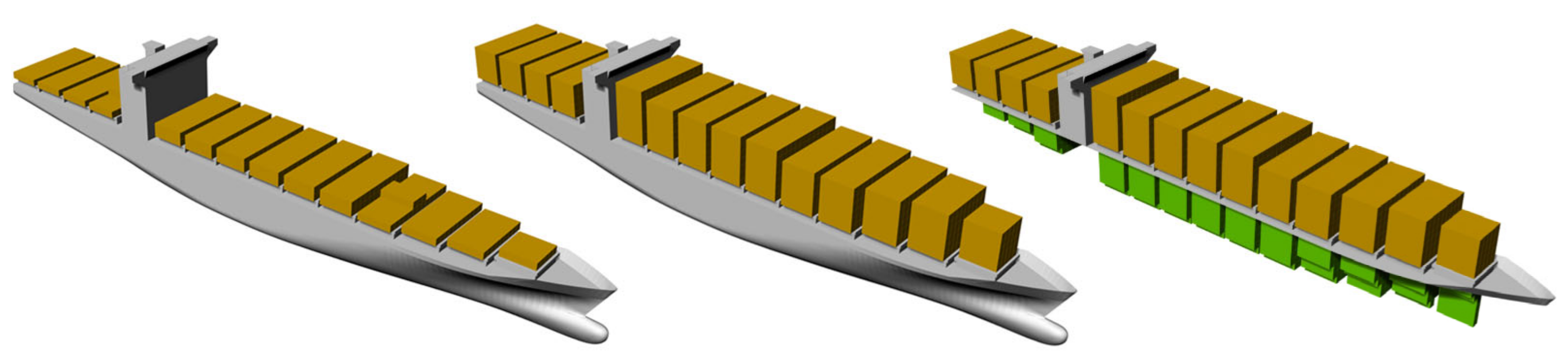
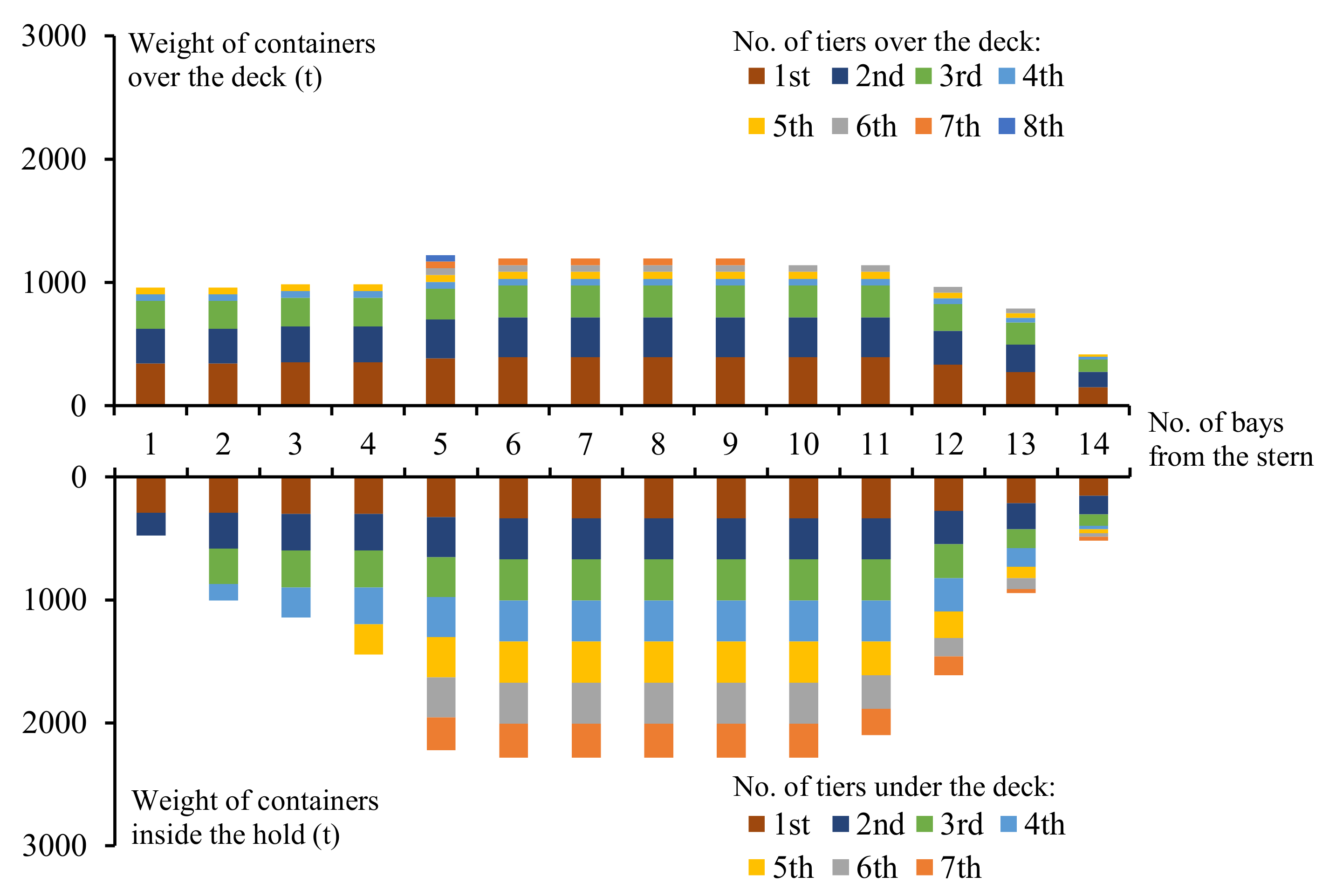
4.1. Design of the Over-Deck Objects

KCS is a 3600 TEU (twenty-foot equivalent unit) container ship with a ship length of 230 (m). In this study, the KCS in EK, that is, the full-load and even keel conditions, were designed to load 1800 FEU (forty-foot equivalent unit (FEU) dry containers (12.192 (m) × 2.438 (m) × 2.591 (m)). The minimum weight per container was assumed as 3.74 (t) for an empty container (self-weight of a container), and the maximum weight was assumed as 30.48 (t) for a full-load container. The total weight of the containers was considered as the weight after excluding the lightweight, which was assumed to be 16,323 (t), from the displacement. The container arrangement and container weight distribution were designed considering the available space in the hold and on deck, the prescribed draft, trim, longitudinal position of the C.G. and its height position to achieve a positive GM. The maximum height of the stacked containers was adjusted to ensure the visibility from the bridge.

Figure 2 illustrates 3D images of the KCS loading containers, that is, S-EK, EK, and EK without the hull image under the deck. Figure 3 shows the weight of the containers on each tier at each bay below the deck (inside the hold) and over the deck in the case of EK; the x-axis indicates the number of container bays in the longitudinal position from the stern, and the legend indicates the number of tiers from the deck. For example, the data x = 6 and “3rd” in the upper figure represent the total weight of the containers positioned on the third tier above the deck at the sixth bay. In the hold, the containers were reduced in the area close to the bow and stern because of the narrow hull width. This resulted in a reduced container weight in that area. Because of the GM, the number of containers on the higher tier over the deck was also small. For TB and TS, which had the same displacement as EK, their weight distribution was designed to achieve the prescribed trim and the proper position of the centre of gravity, assuming the same number of containers, i.e., 1800 FEU, were loaded, and their arrangement was maintained in the same manner as EK. An overloading condition, D-EK, was achieved by arranging overweight containers, of which the per unit weight was assumed to be 1.2-times heavier than a full-load container inside the hold. Meanwhile, S-EK reduced the number of containers to 1025 FEU because of the small displacement, and the arrangement of the containers and their weight distribution were adjusted. Figure 4 shows a comparison of the weight distributions of the containers in the longitudinal direction among the five loading conditions designed in this study.

The radiuses of gyration, $k_{xx}$ and $k_{zz}$, i.e., the moments of inertia of the ship around the $x$ and $z$ axes, were calculated based on the weight distribution of containers in each condition, assuming that those of the naked hull were 0.25 $L$ and 0.25 $B$, respectively. They are listed in

Table 4. Position of the centre of gravity, $\overline{\mathit{GM}}$ and radiuses of gyrations of the ship.

Symbol	S-EK	TS	EK	TB	D-EK
$x_G \left[\mathrm{m}\right]$	−2.17	−7.77	−3.41	0.50	−4.86
$\overline{KG} \left[\mathrm{m}\right]$	11.86	14.67	14.32	14.26	14.70
$\overline{GM} \left[\mathrm{m}\right]$	3.03	0.60	0.63	0.40	0.36
$k_{xx}/B$ [-]	0.329	0.382	0.378	0.378	0.374
$k_{zz}/L$ [-]	0.238	0.246	0.246	0.234	0.247

, along with the position of the C.G. of the ship where $\overline{\mathit{KG}}$ is its height from the keel, and $\overline{\mathit{GM}}$ is the metacentre height. The vertical position of the C.G. of the naked hull was assumed to be half of the draft.

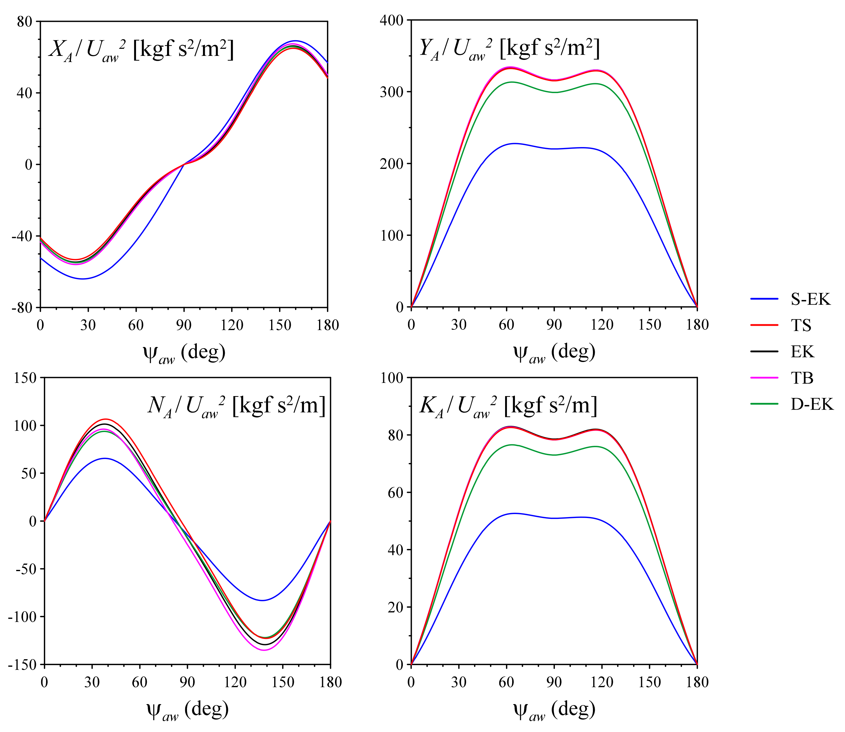
4.2. Estimation of Wind Forces and Moments

Table 5. Representative parameters related to the windage area.

Symbol	S-EK	TS	EK	TB	D-EK
$A_F$ [m2]	1234	1182	1198	1212	1159
$A_L$ [m2]	3934	5665	5676	5670	5391
$C_{MC}$ [m]	−5.40	−2.83	−4.64	−6.37	−4.78
$H_C$ [m]	9.29	13.27	13.31	13.36	12.76

lists the main parameters related to the windage area under each loading condition. $C_{MC}$ is the longitudinal coordinate of the centre of the projected lateral windage area from the midship, and $H_C$ is its height from the waterline. These are important for the yaw and roll moment levers. Because of the same arrangements of containers on the deck among EK, D-EK, TB, and TS (notably, the weight distribution of containers among them was different), there was no significant difference in the lateral windage area, $A_L$. On the other hand, S-EK had a smaller lateral windage area because of the small number of containers on the deck. The frontal windage area, $A_F$, was nearly the same because of the common superstructure, which was the tallest structure on board. The wind force in the longitudinal and lateral directions, $X_A$, $Y_A$, and wind moment in the yaw and roll, $N_A$, $K_A$, were estimated by Fujiwara et al. [22].

The parameters were divided by $U_{aw}^2$ to eliminate the effect of the wind speed and identify the difference due to the difference in the windage area. Figure 5 shows these values against the apparent wind angle ${\psi }_{aw}$. The wind surge force and yaw moment varied to achieve their peaks when the apparent wind blew diagonally in forward or backward directions, whereas the wind lateral force and roll moment appeared larger when the wind blew from the side around ${\psi }_{aw}$ = 90°. The magnitudes of the wind force and moment were proportional to the frontal and lateral windage areas.

5. Validation of the Manoeuvring Mathematical Model

Since the manoeuvring mathematical model of the subject ship was already validated in [5], some representative results are introduced here. The $\pm 35$ (°) turning tests were simulated, and their trajectories are compared with the experimental results in Figure 6. The initial ship speed was 0.86 (m/s). Evidently, the simulation results were able to capture the difference in trajectories due to the difference in draft and the difference in trim observed in the experimental results, thus confirming the validity of the manoeuvring mathematical model of the subject ship.

6. Course-Keeping Simulation

In the previous study [4], the authors discussed the influence of loading conditions on course stability based on eigenvalue analysis, considering the linear hydrodynamic force terms acting on the hull. It was found that even a slight change in the draft and trim from the standard EK impacted the course stability. In this study, a course-keeping simulation was executed to investigate how the ship manoeuvres according to the loading conditions and how the motion changes depending on the wind disturbances. PD (Proportional-Derivative) control with respect to the heading angle and yaw rate was adopted. All calculations were conducted on a real scale. The total resistance coefficient was calculated using a three-dimensional extrapolation method, considering the viscous resistance based on the Reynolds number of the real-scale ship. The wake fraction factor of the scaled model was also converted to a real-scale value using the ITTC formula [24].

6.1. No True Wind Conditions

First, only the wind due to self-propulsion was considered, that is, the no true wind condition. The situation in which the ship with the initial heading angle (${\psi }_0$) of 5 (°) at the initial ship speed ($U_0$) of 24 (kt) attempted to adjust the heading angle to 0 (°) using the PD controller was considered. Figure 7 shows the time series of the heading angle ($\psi$) of the ship under different loading conditions, where the black line shows the result of the proportional control, that is, proportional gain 1 and derivative gain 0. Because this is the most basic steering pattern, the ship’s inherent course stability was intensely reflected in the resultant manoeuvring motions.

The initial heading angle converged in EK, S-EK, and TS. Notably, it converged soon in the case of S-EK. Meanwhile, it gradually diverged in the deep-draft condition, D-EK, and the trim by bow condition, TB. The authors previously discussed the influence of the loading conditions (i.e., draft and trim) on the manoeuvring force and the resultant course stability based on eigenvalue analysis [4], where the course stability tended to deteriorate as the ship’s draft depended or the trim by bow became larger. These characteristics can be confirmed from the results of the simulations. The red line shows the result of the PD control, where both the P and D gains were set to 1. In general, the derivative gain acted as a damper, and the oscillation was suppressed. Indeed, the heading angles in D-EK and TB converged successfully.

In conclusion, it becomes difficult for the operator to manoeuvre the ship in a deep-draft condition (D-EK) or in a trim-by-bow condition (TB). However, it seems possible to manoeuvre the ship stably by considering a derivative control, that is, quick and sensitive steering against the disturbance of motions, so that the overshoot angle is suppressed and the ship can run on the target course smoothly.

6.2. Influence of the Ship Speed and True Wind Angle

This section focuses on EK under true wind conditions. The black line in Figure 8 shows the result of the course-keeping simulation where the ship with ${\psi }_0$ = 5 (°) attempted to maintain the course through PD control while running at $U_0$ = 24 (kt) under the true wind condition of $U_w$ = 9.26 (m/s) and ${\psi }_w$ = 90 (°). Both the proportional and derivative gains were set to one. Owing to its high speed, the rudder force seemed enough to countermeasure the wind force. Thus, the initial disturbances of the motions converged smoothly. The red line represents the simulation results of the ship at $U_0$ = 6 (kt), which was assumed as the harbour speed under the same wind conditions. Focusing on the yaw rate ($r^{\prime }$), a longer time was required for the initial disturbance to converge because the rudder force became small, owing to the small inflow velocity when moving slowly. The rudder angle ($\delta$) changed more dynamically and reached a larger value than in the case of 24 (kt) after the yaw motion was converged. The resultant hull drift angle ($\beta$) also increased in the negative direction. When running at 24 (kt), the roll angle ($\varphi$) was larger than 6 (kt), which may have been due to the larger roll moment induced by the wind because of the faster apparent wind speed. The blue and green lines show the simulation results where $U_0$ = 6 (kt), $U_w$ = 9.26 (m/s) and ${\psi }_w$ = 45 (°) and 135 (°), respectively. By comparing these lines and the red line, the influence of the true wind angle on the course-keeping performance can be discussed. Because of the heading wind when ${\psi }_w$ = 45 (°), the air drag increased with an increase in the apparent wind speed. Thus, a drop in the surge speed ($u^{\prime }$) and the resultant increase in the hull drift angle were observed. The opposite tendency was observed when ${\psi }_w$ = 135 (°) where the wind blew to the ship from the behind, that is, following the wind condition.

Notably, the heading and hull drift angles did not coincide. This indicates that the ship drifted downwind. To maintain a straight course without any deviation, PD control for the lateral displacement should be considered. This is discussed in detail in Section 6.4.

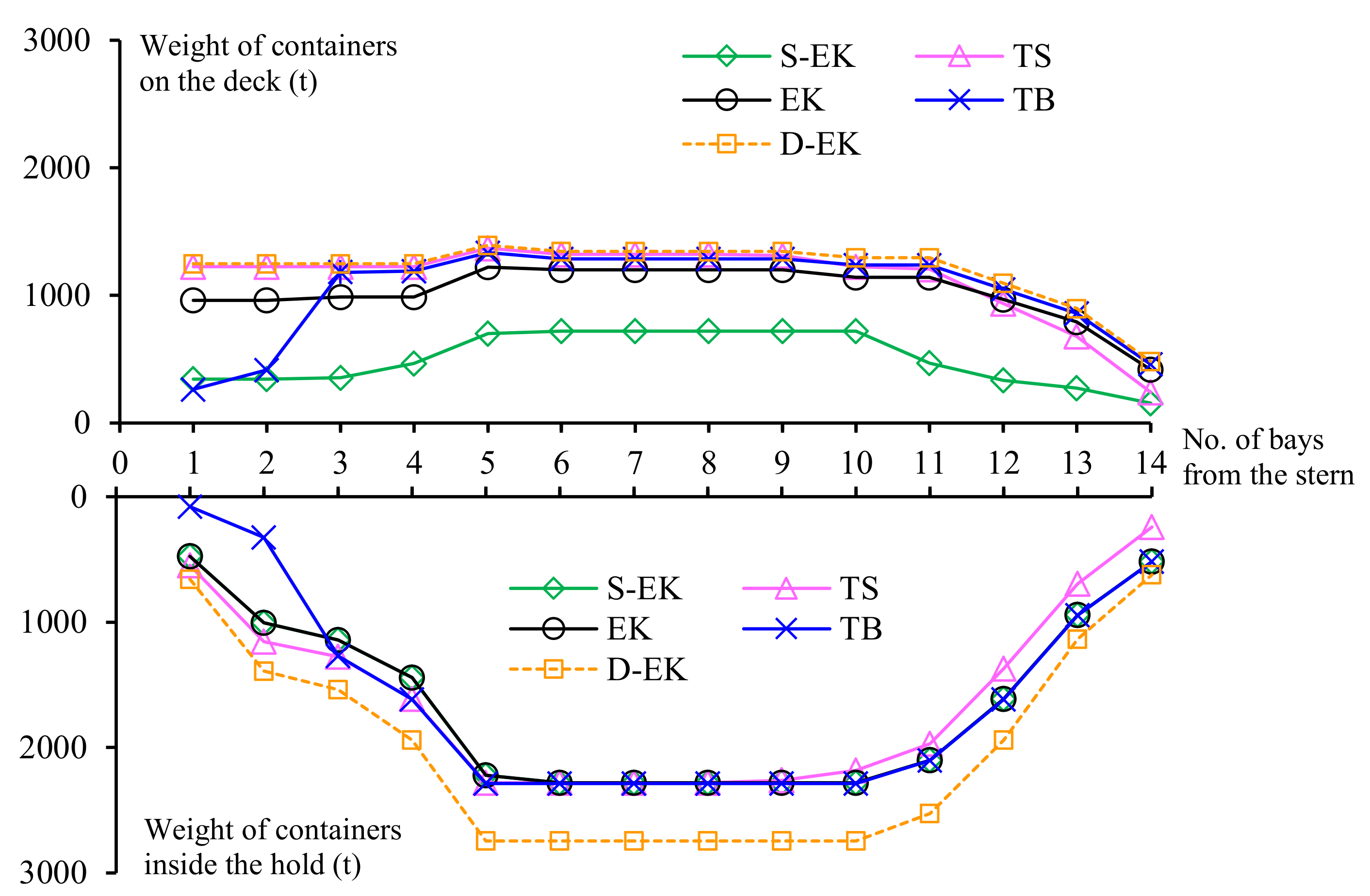
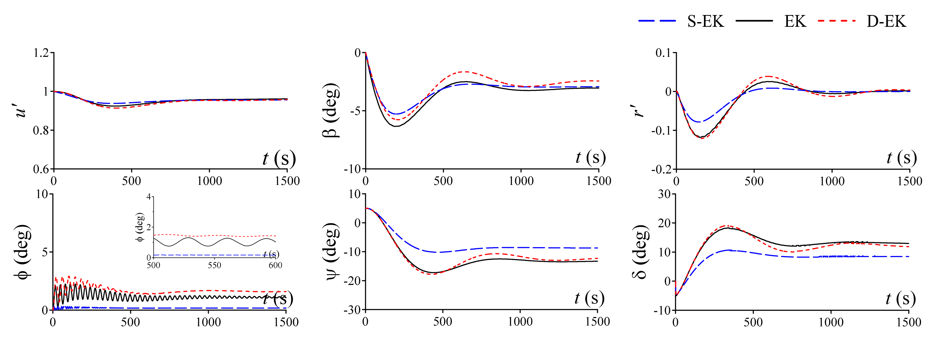
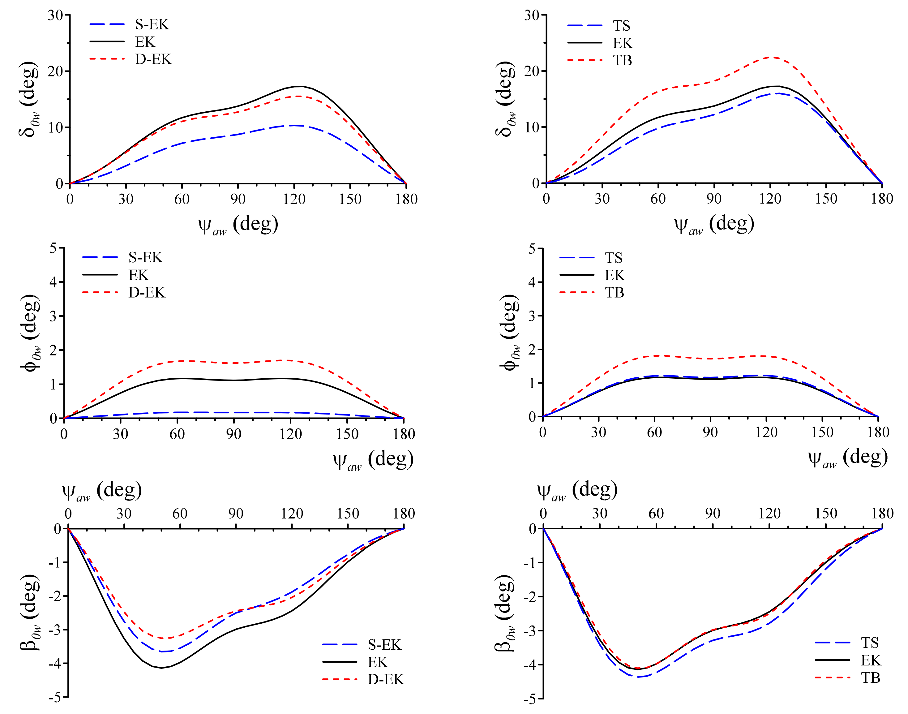
6.3. Influence of Trim and Draft Conditions

Figure 9 shows the results of the draft series, EK, S-EK, and D-EK, where they run at $U_0$ = 6 (kt) with ${\psi }_0$ = 5 (°) under the true wind condition, i.e., $U_w$ = 9.26 (m/s) and ${\psi }_w$ = 90 (°), using both the proportional and derivative control gains 1. S-EK, which had a small windage area owing to the small number of containers, demonstrated a remarkable difference from EK and D-EK. D-EK, which had a larger displacement or inertia force, had larger oscillation in motion than EK.

Figure 10 shows the results of the trim series, EK, TB, and TS, in the same situation as that in Figure 9. The oscillation of the motions was larger in TB, which was characterized as a loading condition with unstable course stability. The yaw rate increased quickly, and the resultant motions tended to be overshot. This indicates that sensitive steering against the ship motions, which implies an increase in the derivative control gain, is important for steady navigation. Compared to D-EK, which also had unstable course stability, the large roll motion continued longer in TB. This was because the submerged hull of TB was smaller than that of D-EK, causing a small damping of the roll motion. When the ship takes the trim by bow, such unstable course stability and large continuous roll motions should be carefully considered.

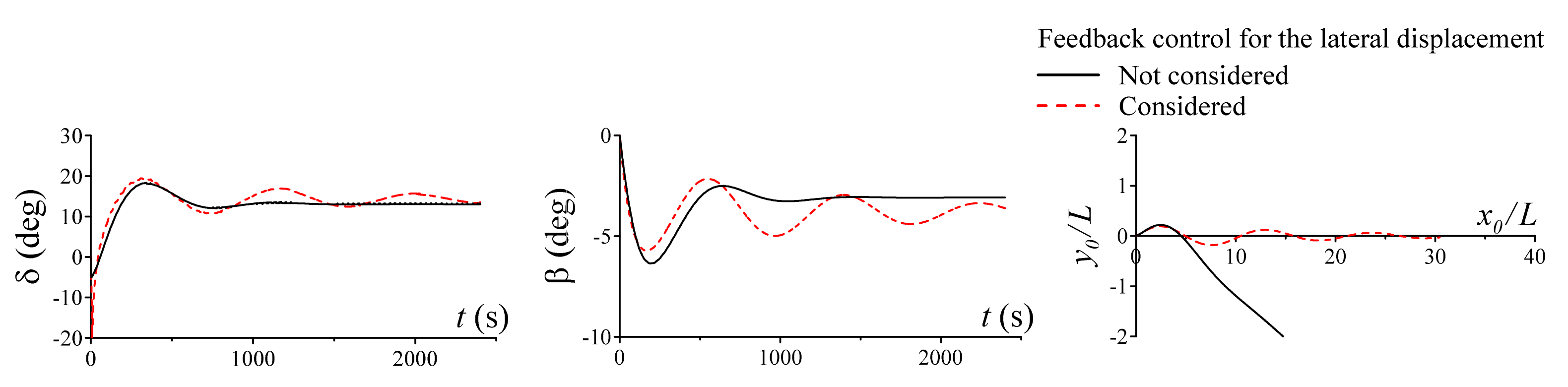
6.4. PD Control Designed to Maintain the Straight Course

As discussed in Section 6.2, the autopilot based on PD control for yaw motion could not stop drifting downwind under wind pressure. Therefore, to maintain a straight course, PD control for the lateral displacement was additionally considered. As an example, Figure 11 shows the states of EK while performing course keeping by the PD control with and without considering the feedback gains for the lateral displacement and its time derivative, that is, the lateral velocity. The initial conditions were ${\psi }_0$ = 5 (°) and $U_0$ = 6 (kt), and true wind conditions were $U_w$ = 9.26 (m/s) and ${\psi }_w$ = 90 (°).

In the case of no consideration, that is, the PD control only for yaw motion with control gains of 1, the ship’s track gradually deviated from the original course (the $x$-axis). On the other hand, in the case of consideration, that is, the PD control for yaw and lateral displacement whose gains were tuned properly, the ship was able to maintain a straight course through steering dynamically. The resultant hull drift angle appears to be larger than that in the case without consideration.

7. Equilibrium State under Wind

An equilibrium state under wind is defined as the steady state while maintaining an original straight course without any deviation, wherein every external force and moment are balanced. The check helm angle (rudder angle), hull drift angle, and roll angle in the equilibrium state were identified based on course-keeping simulations. The PD control for yaw and lateral displacement was considered to avoid deviation from the original course. Each control gain was tuned for this purpose.

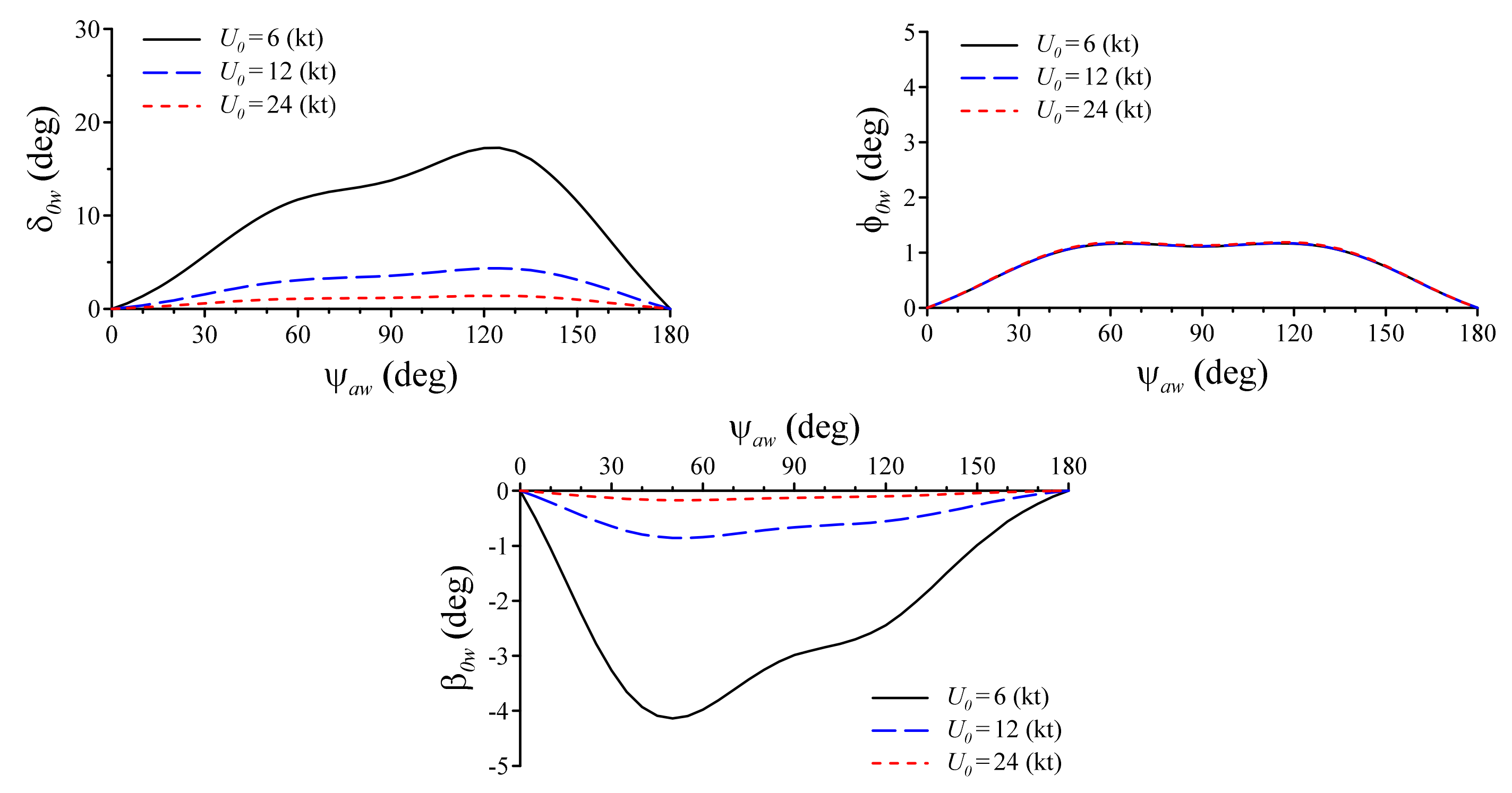
7.1. Influence of the Apparent Wind Speed under the Constant Ship Speed

EK sailing at a constant speed of $U_0$ = 6 (kt), assuming navigation near a coast or harbour, was considered. At such a slow speed, the influence of the wind on the ship’s manoeuvrability was relatively strong. Figure 12 shows the check helm (${\delta }_{0w}$), hull drift (${\beta }_{0w}$), and roll angles (${\varphi }_{0w}$) in the equilibrium state with respect to the apparent wind angle from 0 (°) to 180 (°). The three lines in each subfigure represent the results of the different ratios of the apparent wind speed to the ship speed, that is, 1, 2, and 3. For example, in the case of $U_{aw}/U_0=3$, the true wind speed ($U_w$) was equivalent to the Beaufort scale (BF) from 4 to 6, that is, a moderate breeze (BF4) at ${\psi }_{aw}=0^{°}$ and strong breeze (BF6) at ${\psi }_{aw}={180}^{°}$.

The result of $\frac{U_{aw}}{U_0}=1$ indicates that each angle required for course-keeping increased when the apparent wind blew against the hull from the side. Their angles drastically increased with an increase in the apparent wind speed; for example, in the case of $U_{aw}/U_0=3$ and ${\psi }_{aw}=90$ (°), the check helm angle was 13.8 (°), in spite of only 1.4 (°) in the case of $U_{aw}/U_0=1$ and the same ${\psi }_{aw}$ as above. In particular, the largest check helm angle was required at approximately ${\psi }_{aw}$ = 125 (°). As shown in Figure 5, a lateral wind force exhibited a positive peak around this wind angle, which caused the ship to drift away in the starboard direction (see the coordinate system in Figure 1). In addition, a large negative moment in yaw caused by the wind caused the ship to turn in the counter-clockwise direction. Thus, the ship requires a large positive check helm angle which moves it in the port direction and a clockwise moment to maintain balance.

However, the absolute hull drift angle showed the largest angle around ${\psi }_{aw}=50$ (°) at which the large lateral wind force to the starboard and clockwise wind moment acted on the ship. To reduce the starboard movement, a positive rudder angle is required to generate a rudder force in the port direction. Because the direction of the yaw moment due to the rudder force is clockwise and in the same direction as that due to the wind force, the ship must take the negative hull drift angle to cancel these yaw moments by the hydrodynamic yaw moment acting on the hull. Therefore, the peak of the hull drift angle appeared around this apparent wind angle.

The roll angle in the equilibrium state did not exhibit a significant peak. Equation (2) signifies that it was influenced by the rudder force ($Y_R$), which correlated with the rudder angle and reached a maximum around ${\psi }_{aw}$ = 125 (°), and the hull force ($Y_H$), which correlated with the hull drift angle and reached a maximum value around ${\psi }_{aw}$ = 50 (°). Because of the apparent wind angle around which $Y_H$ and $Y_R$ peak did not overlap, the roll angle tended to be flat without any significant peaks and achieved a small value overall.

7.2. Influence of the Ship Speed under the Constant Apparent Wind Speed

Assuming the apparent wind speed to be constant, $U_{aw}$ = 9.26 (m/s), the equilibrium states of EK at ship speeds of $U_0$ = 6, 12, and 24 (kt) are shown in Figure 13, where the apparent wind angle is taken as the horizontal axis. Notably, the results for $U_0$ = 6 (kt) are the same as those for $U_{aw}/U_0=3$ in Figure 12.

When the ship speed was high, the check helm angle became significantly smaller. This appears to be because the propeller rotation speed for self-propelling increased when the ship speed was high. This caused the flow speed at the rudder to become much faster, resulting in a larger rudder force. Similarly, the hull drift angle was also affected by the speed of the ship. Because the hydrodynamic force acting on the hull increased as the ship speed increased, and even a small hull drift angle could be balanced by the wind moment. Meanwhile, the influence of the ship speed on the roll angle was not significant. This may be because the direction of the hull force, $Y_H$, and rudder force, $Y_R$, were opposite, and the increments of both forces associated with the increase in ship speed may have cancelled each other.

These results indicate that one must be careful of an expected large check helm and the ship’s attitude for course keeping when navigating a harbour or coastal areas in which the ship speed is commonly slow. However, it is also possible to reduce these values by slightly increasing the ship speed under such circumstances. Thereby, a greater safety margin for manoeuvring could be expected. When sailing at a navigation speed of 24 (kt), the ship is supposed to be able to maintain the course with a sufficiently small check helm and hull drift angles under the wind conditions considered here.

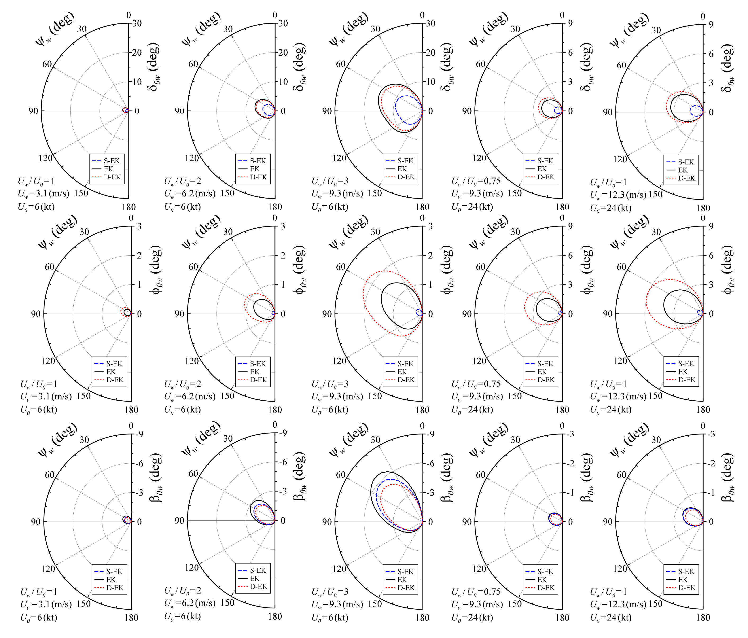
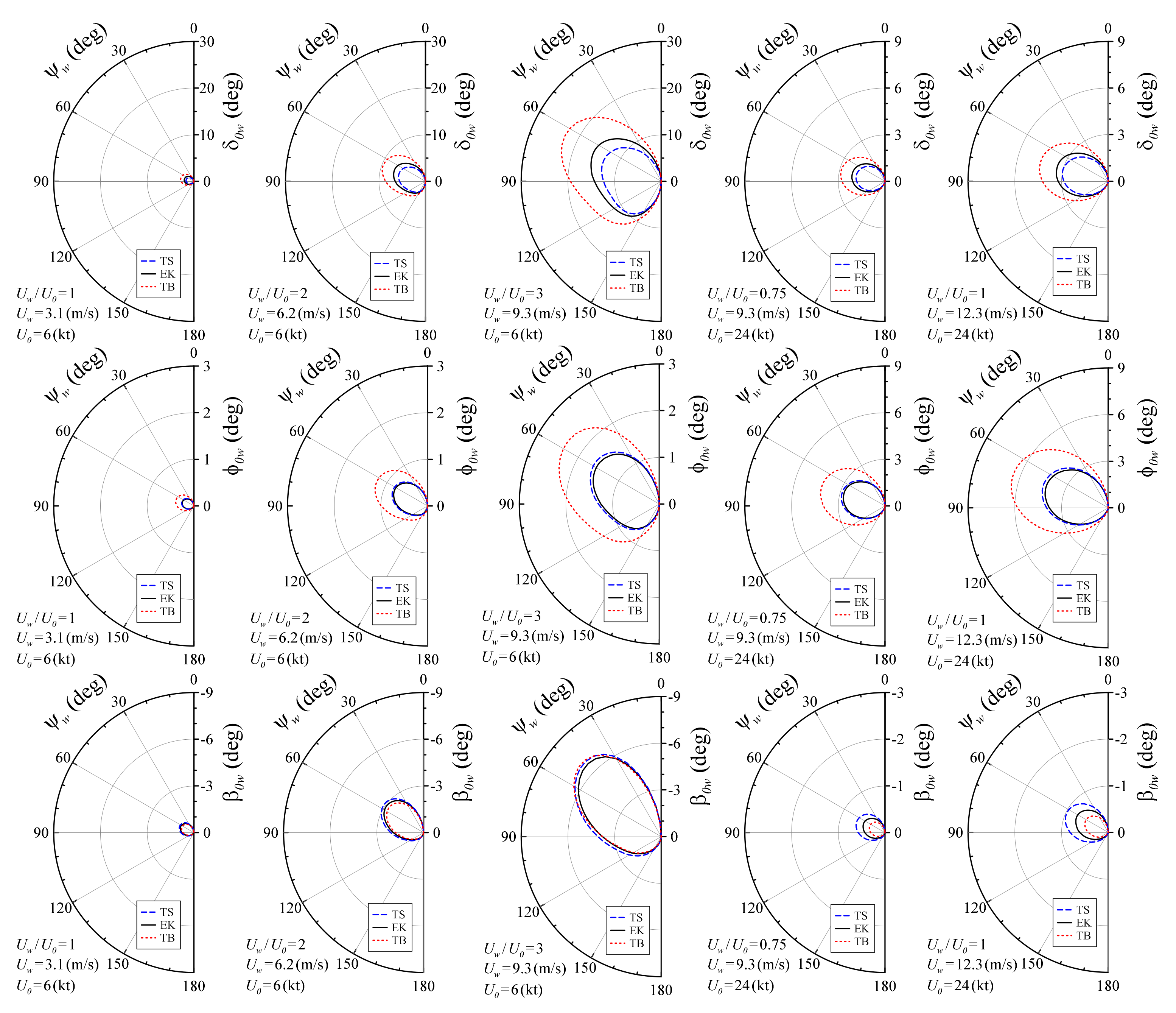
7.3. Influence of the Loading Condition under the Constant Ratio of the Apparent Wind and Ship Speeds

The influence of the loading conditions on the equilibrium states was investigated. The apparent wind speed was assumed to be $U_{aw}$ = 9.26 (m/s), whereas the ship speed was $U_0$ = 6 (kt). The results of the draft series are arranged on the left, and those of the trim series are shown on the right in Figure 14.

Focusing on the draft series, the check helm angle of S-EK was smaller than that of EK. This resulted from the small windage area, owing to the small number of containers, as shown in Figure 2. It seems that D-EK requires a slightly smaller check helm angle than EK. Because of the deeper draft and larger drag, a higher propeller rotational speed, in which a larger rudder force is expected, is required for self-propelling. Thus, even a small check helm angle may have been enough. The hull drift angles of S-EK and D-EK were smaller than those of EK. The reason for this difference can be discussed in the same way as above. The roll angle for course keeping under the same apparent wind angle seemed to increase in the order of S-EK, EK, and D-EK. The significant small roll angle of S-EK was due to the large GM because of the low position of the centre of gravity. On the other hand, the large roll angle of D-EK was due to the small GM, as listed in Table 4.

Focusing on the check helm angle in the trim-series condition, the ship with the trim by bow required a larger check helm angle, that is, 22.5 (°) in TB, 17.3 (°) in EK, and 16 (°) in TS around ${\psi }_{aw}=125$ (°). The authors’ previous study [4] presented the rudder force and resultant rudder moment increase in the order of TB, EK, and TS. They were correlated with the propeller rotation speed for self-propulsion, owing to their resistance and self-propulsive performance. Because TB ran at a lower propeller load, it needed to take a larger check helm angle to increase the rudder force to balance the wind force. In terms of the hull drift angle in the equilibrium state, TS had a larger absolute value overall. As discussed in [4], because of the deep draft at the stern in TS, the acting point of the hull drift force, which was positioned at the fore of the hull, moved backward toward the midship. This resulted in a smaller yaw damping moment in hull drift conditions. Therefore, a large hull drift angle is required to balance the yaw moment caused by wind. Meanwhile, the influence of the loading conditions on the roll angle in the equilibrium state can be explained by the difference in the GM. In the case of TB, in which the draft at the stern was shallow, the hull shape around the stern under water became thin, which resulted in a smaller second moment of the water surface area than EK and TS. Because the radius of the metacentre was proportional to this moment of area, the vertical position of the metacentre was lower, resulting in the smaller GM. It caused the large roll angle of TB.

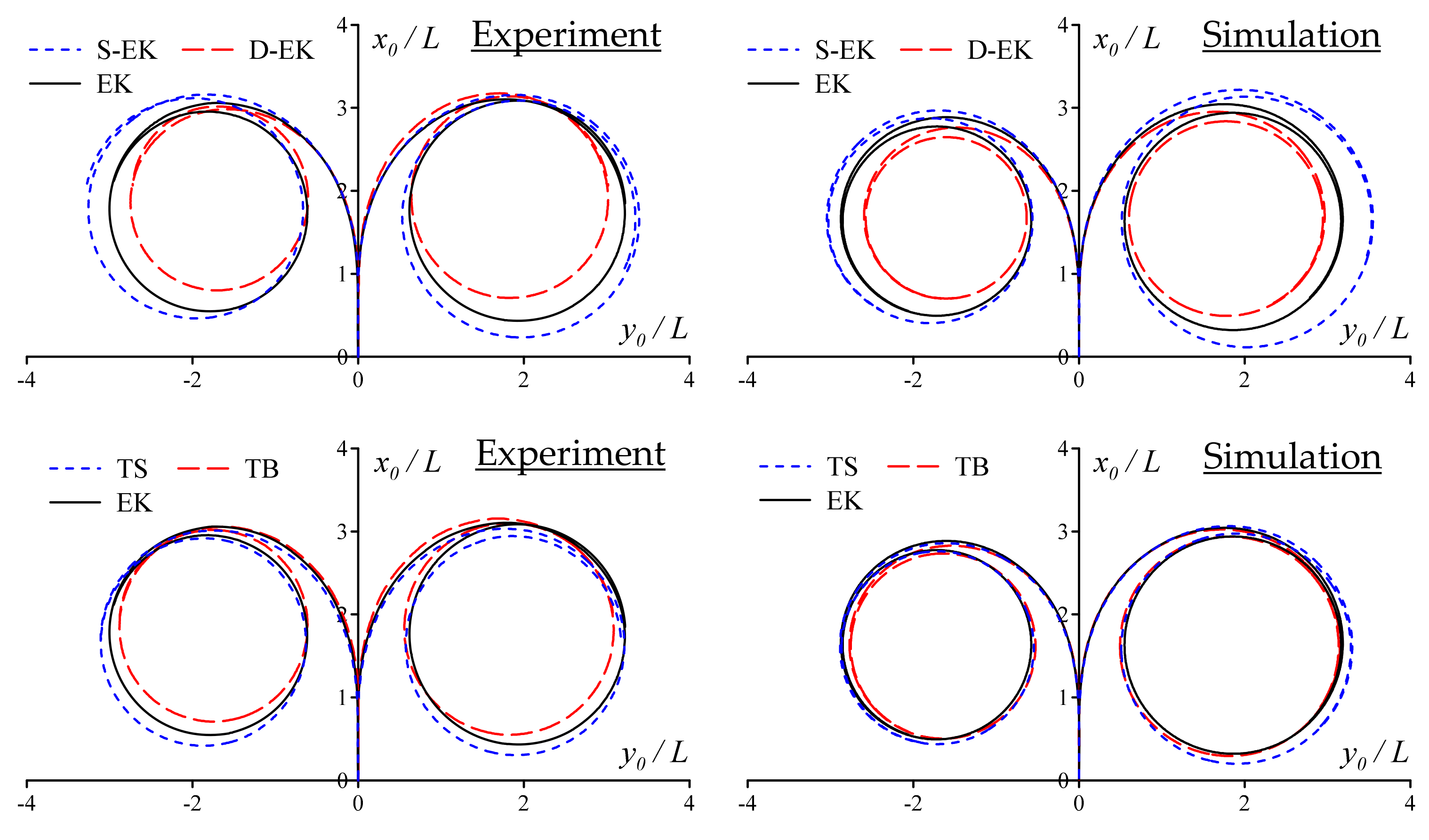
7.4. Discussion of the Equilibrium State Based on the Polar Chart

Although discussions based on apparent wind, defined as the sum of head wing that a running ship faces and true wind, are useful for immediate knowledge, it may be difficult to know which direction the true wind blows against the ship and how fast the true wind blows. Therefore, in this section, a polar chart of the equilibrium state is illustrated based on the true wind direction and speed. This chart has the advantage of allowing users to intuitively grasp the relationship between their ship speed, true wind conditions, and the resultant equilibrium states of the ship. The results of the draft series are shown in Figure 15.

The check helm, roll, and hull drift angles in the equilibrium state were plotted in polar charts, where the direction of the angle of the true wind was taken in the circumferential direction. The subfigures arranged in the first, second, and third columns show the results when the ship ran at $U_0$ = 6 (kt) under the wind condition in which the true wind speeds were $U_w$ = 3.1, 6.2 and 9.3 (m/s). These are equivalent to the ratio of the true wind speed to the ship speed, that is, $U_w/U_0$ = 1, 2, and 3. In these cases, the check helm angle reached maximum when the true wind blew against the ship from diagonally forward, that is, around ${\psi }_w$ = 70 (°). A similar trend was observed for every loading condition, and the order of magnitude of each absolute angle was the same as in the discussion in Figure 14. In the fourth column in Figure 15, the results of the condition where the ship speed was $U_0$ = 24 (kt) and the speed of the true wind was $U_w$ = 9.3 (m/s) are shown. The speed effect on the equilibrium state can be observed by comparing the results of the third and fourth columns. With an increase in the ship speed, the ring size illustrated on the polar chart significantly shrunk because of the expected larger rudder force, indicating that the ship could maintain the course with a small check helm angle without a large change in the ship’s attitude. The fifth column shows the results when the ship speed was $U_0$ = 24 (kt) and the true wind speed was $U_w$ = 12.3 (m/s). Notably, the only difference from the fourth column is the speed of the true wind blowing against the ship. Although the ring size increased, this ship could maintain its course at 24 (kt) even under a strong breeze (BF 6), regardless of the draft condition.

Figure 16 shows the results for the trim-series condition. Although the almost same consideration can be made as in Figure 15, a unique phenomenon was observed in the case of $U_w=9.3$ (m/s) and $U_0=6$ (kt), only in which the ring size of the hull drift angle of TB was as large as that of TS. Because it is the case of $U_w/U_0=3$ that the wind effect on the ship motions is stronger than other cases, the check helm angle increased overall. As can be seen from Figure 16, since TB tended to take a larger check helm angle than TS, the larger surge-speed drop was expected due to the larger steering drag, especially under such a strong wind. It caused the influence of the sway motion to be relatively large and resulted in the increase of the hull drift angle of TB.

8. Conclusions

The loading conditions and wind effects on the course-keeping performance of the 3600TEU-loaded container ship were investigated. The windage section on the upper deck was designed under five loading conditions which had various draft and trim combinations, and the wind forces and moments acting on the ship were estimated. Based on the developed mathematical model, the course-keeping performance under wind was investigated by simulation. The main conclusions are summarized as follows.

• The check helm angle under wind conditions, which is defined as the rudder angle required to maintain the specified course without deviation, was significantly different among the loading conditions. Meanwhile, the difference in the hull drift angle and roll angle in the equilibrium state was relatively small among them.
• In all cases, maintaining the specified course straight when a wind blew diagonally from behind was the most severe condition, wherein the largest check helm angle was required, and the steering margin was reduced.
• Among the trim-series conditions, the trim by bow required a larger check helm angle, while the trim by stern had a smaller angle. This is related to the essential course stability determined by the hydrodynamic water forces acting on the hull under each loading condition.
• A shallow-draft ship requires a significantly small check helm angle. This is because of the small windage area as well as the better course stability.
• An increase in ship speed is an effective way to reduce the check helm angle by increasing the rudder force.
• A polar chart of the equilibrium state was presented based on the true wind direction and speed. This type of chart has the advantage of allowing users to intuitively grasp the relationship between their ship speed, true wind conditions, and the resultant equilibrium states of the ship.

References

1. RESOLUTION MSC.137(76): Standards for Ship Manoeuvrability. Available online: https://wwwcdn.imo.org/localresources/en/KnowledgeCentre/IndexofIMOResolutions/MSCResolutions/MSC.137(76).pdf (accessed on 9 April 2023).
2. Islam, H.; Soares, C.G. Effect of trim on container ship resistance at different ship speed and drafts. Ocean Eng. 2019, 183, 106–115. [Google Scholar] [CrossRef]
3. Reichel, M.; Minchev, A.; Larsen, N.L. Trim optimization—Theory and practice. TransNav 2014, 8, 387–392. [Google Scholar] [CrossRef]
4. Himaya, A.N.; Sano, M.; Suzuki, T.; Shirai, M.; Hirata, N.; Matsuda, A.; Yasukawa, H. Effect of the loading conditions on the maneuverability of a container ship. Ocean Eng. 2022, 247, 109964. [Google Scholar] [CrossRef]
5. Yasukawa, H.; Himaya, A.N.; Hirata, N.; Matsuda, A. Simulation study of the effect of loading condition changes on the maneuverability of a container ship. J. Mar. Sci. Technol. 2023, 28, 98–116. [Google Scholar] [CrossRef]
6. Zhou, Y.; Daamen, W.; Vellinga, T.; Hoogendoorn, S.P. Impacts of wind and current on ship behavior in ports and waterways: A quantitative analysis based on AIS data. Ocean Eng. 2020, 213, 107774. [Google Scholar] [CrossRef]
7. Yoshimura, Y.; Nagashima, J. Estimation of the manoeuvring behaviour of ship in uniform wind. J. Soc. Nav. Archit. Jpn. 1985, 158, 125–136. (In Japanese) [Google Scholar] [CrossRef] [PubMed]
8. Hasegawa, K.; Kang, D.H.; Sano, M.; Nagarajan, V.; Yamaguchi, M. A study on improving the course-keeping ability of a pure car carrier in windy conditions. J. Mar. Sci. Technol. 2006, 11, 76–87. [Google Scholar] [CrossRef]
9. Nagarajan, V.; Kang, D.H.; Hasegawa, K.; Nabeshima, K. Comparison of the mariner Schilling rudder and the mariner rudder for VLCCs in strong winds. J. Mar. Sci. Technol. 2008, 13, 24–39. [Google Scholar] [CrossRef]
10. Paroka, D.; Muhammad, A.H.; Asri, S. Maneuverability of ships with small draught in steady wind. Makara J. Technol. 2016, 20, 24–30. [Google Scholar] [CrossRef]
11. Im, N.K.; Tran, V.L. Ship’s maneuverability in strong wind. J. Navig. Port Res. Int. Ed. 2008, 32, 115–120. [Google Scholar] [CrossRef]
12. Lee, C.K.; Lee, S.G. Hydrodynamic forces between vessels and safe maneuvering under wind-effect in confined waters. J. Mar. Sci. Technol. 2007, 21, 837–843. [Google Scholar] [CrossRef]
13. Silva, A.S.; Oleinik, P.H.; Kirinus, E.P.; Costi, J.; Guimaraes, R.C.; Pavlovic, A.; Marques, W.C. Preliminary study on the contribution of external forces to ship behavior. J. Mar. Sci. Eng. 2019, 7, 72. [Google Scholar] [CrossRef]
14. Andersen, I.M.V. Wind loads on post-panamax containership. Ocean Eng. 2013, 58, 115–134. [Google Scholar] [CrossRef]
15. Janssen, W.D.; Blocken, B.; Wijhe, H.J. CFD simulations of wind loads on a container ship: Validation and impact of geometrical simplifications. J. Wind. Eng. Ind. Aerodyn. 2017, 166, 106–116. [Google Scholar] [CrossRef]
16. Seok, J.; Park, J.C. Comparative study of air resistance with and without a superstructure on a container ship using numerical simulation. J. Mar. Sci. Eng. 2020, 8, 267. [Google Scholar] [CrossRef]
17. FORCE Technology and Iowa Institute of Hydraulic Research (IIIHR) Part B: Benchmark Test Cases, KCS Description. In Proceedings of the Workshop on Verification and Validation of Ship Manoeuvring Simulation Methods (SIMMAN2008), Copenhagen, Denmark, 14–16 April 2008; pp. B11–B14.
18. Lee, S.J.; Koh, M.S.; Lee, C.M. PIV velocity field measurements of flow around a KRISO 3600TEU container ship model. J. Mar. Sci. Technol. 2003, 8, 76–87. [Google Scholar] [CrossRef]
19. Islam, H.; Soares, C.G. Estimation of hydrodynamic derivatives of an appended KCS model in open and restricted waters. Ocean Eng. 2022, 266, 112947. [Google Scholar] [CrossRef]
20. Hamamoto, M.; Kim, Y.-S. A new coordinate system and equations describing the maneuvering motion of a ship in waves. J. Soc. Nav. Archit. Jpn. 1993, 173, 209–220. (In Japanese) [Google Scholar] [CrossRef]
21. Yasukawa, H.; Yoshimura, Y. Introduction of MMG standard method for ship maneuvering predictions. J. Mar. Sci. Technol. 2015, 20, 37–52. [Google Scholar] [CrossRef]
22. Fujiwara, T.; Ueno, M.; Ikeda, Y. A new estimation method of wind forces and moments acting on ships on the basis of physical component models. J. Jpn. Soc. Nav. Archit. Ocean Eng. 2005, 2, 243–255. (In Japanese) [Google Scholar]
23. ITTC Quality System Manual—Recommended Procedures and Guidelines: Preparation, Conduct and Analysis of Speed/Power Trials. Available online: https://www.ittc.info/media/9874/75-04-01-011.pdf (accessed on 9 April 2023).
24. ITTC Quality System Manual—Recommended Procedures and Guidelines: 1978 ITTC Performance Prediction Method. Available online: https://www.ittc.info/media/8017/75-02-03-014.pdf (accessed on 9 April 2023).
Figure 1. Coordinate systems and definition of variables.
Jmse 11 01052 g001
Figure 2. Images of KCS with loading containers: S-EK (left), EK (middle), EK with visualization of the containers inside (right).
Jmse 11 01052 g002
Figure 3. Weight of containers on each tier at each bay for EK.
Jmse 11 01052 g003
Figure 4. Comparison of the weight distribution of containers in the longitudinal direction among the five loading conditions.
Jmse 11 01052 g004
Figure 5. Estimated wind force and moment with respect to the apparent wind angle.
Jmse 11 01052 g005
Figure 6. Comparison of  ± 35  (°) turning trajectories among draft-series conditions (upper) and trim-series conditions (lower) between the free-running experiment and simulation.
Jmse 11 01052 g006
Figure 7. Influence of the rudder control gains on the convergence of the heading angle when keeping the course under no true wind.
Jmse 11 01052 g007
Figure 8. Influence of the ship speed and true wind angle on the states of EK when keeping the course under wind.
Jmse 11 01052 g008
Figure 9. Comparison of the states while course keeping by PD control among the draft series, i.e., EK, S-EK, and D-EK under wind;  U w  = 9.26 (m/s) and  ψ w  = 90 (°).
Jmse 11 01052 g009
Figure 10. Comparison of the states while course keeping by PD control among the trim series, i.e., EK, TB, and TS under wind;  U w  = 9.26 (m/s) and  ψ w  = 90 (°).
Jmse 11 01052 g010
Figure 11. Comparison of the hull drift angle, rudder angle, and trajectory of EK while course keeping by the PD control for yaw motion (in black) and the PD control for yaw and lateral displacement (in red) under wind;  U w  = 9.26 (m/s) and  ψ w  = 90 (°).
Jmse 11 01052 g011
Figure 12. Equilibrium states of EK sailing at  U 0  = 6 (kt) under different apparent wind speeds, i.e.,  U a w / U 0  = 1, 2, 3.
Jmse 11 01052 g012
Figure 13. Equilibrium states of EK sailing at different ship speeds, i.e., 6, 12, 24 (kt), under the apparent wind speed, i.e.,  U a w  = 9.26 (m/s).
Jmse 11 01052 g013
Figure 14. Equilibrium state of EK, S-EK, and D-EK (draft series) and EK, TB, and TS (trim series) sailing at  U 0  = 6 (kt) under the same apparent wind speed, i.e.,  U a w  = 9.26 (m/s) which corresponds to  U a w / U 0 = 3 .
Jmse 11 01052 g014
Figure 15. Polar chart of the equilibrium states of EK, S-EK, and D-EK (draft series) in various combinations of the true wind and ship speed.
Jmse 11 01052 g015
Figure 16. Polar chart of the equilibrium states of EK, TS, and TB (trim series) in various combinations of the true wind and ship speed.
Jmse 11 01052 g016