Abstract
The deep western boundary current (DWBC) in the Philippine Sea has been expected to play a crucial role in transporting lower circumpolar deep water and to contribute to regional and global climate regulation. Two-year-long near-bottom current measurements reveal a southward-flowing DWBC with a mean velocity of 5 cm/s and seasonal variations—weaker in summer and stronger in winter. Seasonal variability in the DWBC is hypothesized to be induced by changes in the North Equatorial Current bifurcation latitude (NECBL) and upper pycnocline depth through potential vorticity conservation. Data-assimilated reanalysis model (GLORYS12V1) outputs, which reproduce the seasonal variability of DWBC similarly to the observation, are used for further analysis. During the seasonal period, the NECBL displays significant coherence (>0.9) with the first-mode empirical orthogonal function principal component of the simulated along-slope DWBC. The upper pycnocline depth, varying seasonally within a range of approximately 27 m, induces seasonal variability in a deep anticyclonic eddy trapped by topography. In summer, the intensified deep anticyclonic eddy obstructs the adjacent southward-flowing DWBC, weakening its strength, whereas in winter, the southward flow of the DWBC is enhanced due to the weakening of the deep anticyclonic eddy.
1. Introduction
The deep western boundary current (DWBC) flows meridionally, sometimes crossing the equator, along the western side of the deep basin at depths of thousands of meters. In the southwestern Pacific Basin, it flows northward along the western side and transports lower circumpolar deep water (LCDW) from the Southern Ocean to the northwestern Pacific [1]. In the Atlantic Ocean, the DWBC transports cold and saline north Atlantic deep water from the northern Atlantic to the Antarctic Circumpolar Current region [2,3]. Böning and Schott [4] demonstrated that the DWBC in the Atlantic Ocean exhibits seasonal variability, which is related to westward-propagating baroclinic Rossby waves generated by wind stress changes in regions apart from the DWBC area. Despite the critical roles of DWBCs in influencing regional and global climates through meridional heat transport, their features and variability are not well understood, primarily due to the limitations of remote sensing in investigating DWBCs and the lack of in situ measurements. In particular, the study of the DWBC in the northwestern Pacific, which is considered an upwelling region of the global meridional overturning circulation, is insufficient compared to other DWBCs in the global ocean.
The existence, flow direction, and seasonality of the DWBC in the Philippine Sea have yet to be clearly elucidated, although they have been investigated by several previous studies. Stommel and Aron [5] predicted a northward DWBC at the western boundary of the tropical Pacific using theoretical estimations and some in situ measurements. Recently, Zhai and Gu [6] predicted the existence of a northward DWBC as part of an anticyclonic circulation in the southwestern Philippine Basin using numerical model analysis. Conversely, Ishizaki [7] predicted a southward DWBC for the western Philippine Sea using a numerical model. In discontinuous 18-month-long in situ current measurements, Wang et al. [8] discovered a southward DWBC and its seasonal variability, which became stronger in the winter and weaker in early autumn. They demonstrated a seasonally varying relationship between the upper and deep layers, which was supported by a significant correlation. However, no specific physical processes were provided to explain their seasonality.
The North Equatorial Current bifurcation latitude (NECBL) refers to the latitude at which the westward North Equatorial Current (NEC) bifurcates into the Kuroshio Current (KC) and Mindanao Current (MC) when it meets the Philippines. When the NEC bifurcates, the meridional geostrophic velocity near the Philippines vanishes and each portion of transport divided by the NECBL enter the KC and MC, respectively [9,10,11]. The NECBL exhibits evident seasonal variation, being southernmost in summer and northernmost in winter [10,12]. Local wind stress curl and coastal Kelvin waves are known to induce its seasonality [9,12]. Li and Gan [11] explains the seasonal variations of the NEC intensity, meridional migration, and the NECBL in terms of spatiotemporal modes in the NEC transport. When the NEC is intensified with an increase in transport, the NECBL, which is highly correlated with the NEC migration, reaches the southernmost location. The seasonal migration of the NECBL is closely related to the seasonal variability of the pycnocline thickness in the northwestern Pacific. Due to the meridional oscillations of the NECBL, the pycnocline depth of the northwestern Pacific, which deepens northward, also changes seasonally, becoming deeper in summer and shallower in winter [12]. The seasonal variability of the pycnocline is confined to the 1026.7 kg/m3 isopycnal surface [13,14]. Based on this depth, the pycnocline is distinguished into upper and lower pycnoclines.
In this study, we investigated the seasonality of the DWBC using two-year-long in situ near-bottom velocity records collected near the Philippine Trench and data-assimilated numerical reanalysis outputs from GLORYS12V1 that reproduced a realistic DWBC consistent with near-bottom velocity observations. Our focus is mainly on the seasonal migration of the NECBL and seasonal displacement of upper pycnocline occurring in the tropical northwestern Pacific, and we hypothesize that it is a source that can induce the seasonal variability of the DWBC. The displacement of the upper pycnocline thickness caused by the NECBL migration can produce changes in the deep layer thickness, inducing variations in the deep eddy through potential vorticity conservation. Previous numerical model experiments have proven that deep-layer stretching (shrinking) can enhance the counterclockwise (clockwise) anomalies of a deep eddy trapped by bottom topography, e.g., [15,16,17]. We demonstrate highly related features among the DWBC and NECBL, upper pycnocline depth, and a deep eddy simulated by GLORYS12V1, and show that the seasonally varying deep eddy generated by the pycnocline depth change can influence the seasonal variability of the DWBC.
2. Materials and Methods
2.1. Data
An array of three current- and pressure-recording inverted echo sounders (CPIES) was deployed along 8° N in the deep layer of the Philippine Sea from November 2017 to December 2019 (see Figure 1). Mooring sites MP2–MP4 were located at longitudes 127.00° E, 127.65° E, and 128.31° E, respectively, with bottom depths of 4907, 5826, and 4011 m. CPIES is an ocean instrument that can investigate oceanic barotropic and baroclinic variabilities for months to years [18]. The CPIES measures round-trip acoustic travel time, bottom pressure, and single-depth near-bottom velocity. The three pressure-recording inverted echo sounders, deployed on the sea floor of the Philippine Basin, were attached on an anchor stand to prevent movement during the observation. The three current meters, connected to pressure-recording inverted echo sounders, were launched approximately 50 m above the sea floor using a float buoy and recorded near-bottom velocity data with a 30 min interval. The Aanderaa Model 4930R ZPulse Doppler Current Sensor (manufactured by Ananderaa, Bergen, Norway), of which the current sensor head is the same with Aanderaa’s SeaGuard Model Recording Current Meter, was used as a current sensor [19]. The current sensor can measure a velocity in the range of 0–300 cm/s with an absolute accuracy of ±0.15 cm/s and a resolution of 0.01 cm/s [20]. Further description about the mooring system of CPIES can be found in Jeon et al. [18] and User’s Manual [19]. Among the CPIES-measured data, we used near-bottom current records to investigate the variability of abyssal currents.
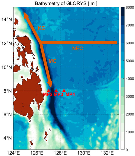
Figure 1.
Bathymetry of GLORYS12V1, schematic of currents in the Philippine Sea, and the locations of near-bottom current meter moorings (red triangles). The contour interval is set as 500 m. NEC represents the North Equatorial Current; KC corresponds to the Kuroshio Current; and MC denotes the Mindanao Current.
The numerical model, GLORYS12V1, provided by the Copernicus Marine Environment Monitoring Service (CMEMS), was also used to analyze the spatial structure and seasonal variability of DWBC in the Philippine Sea. GLORYS12V1, based on the Nucleus for a European Model of the Ocean (NEMO) platform [21], is forced by the atmospheric forcing of 3 h and 24 h ERA-interim from the European Center for Medium-Range Weather Forecasts (ECMWF), which includes precipitation and long and short radiative fluxes. Satellite-measured data, such as the sea surface altimeter, sea surface temperature, sea ice concentration, and in situ temperature and salinity vertical profiles, were assimilated into GLORYS12V1 using a reduced-order Kalman filter [22]. Long-term temperature and salinity biases were corrected using a 3D-VAR scheme [21]. GLORYS12V1 has a 1/12° horizontal resolution and consists of 50 vertical layers following the z coordinates, of which the thickness gradually increases with depth. For this study, we used approximately 14.5-year-long (January 2005–June 2019) three-dimensional daily outputs of temperature, salinity, and horizontal velocity fields in a domain of 3°–18° N and 124°–133° E.
2.2. Methods
To remove high-frequency signals, such as tidal current and inertial waves, the observed hourly near-bottom velocity components () were third-order low-pass filtered with a 48 h cutoff period. The major and minor components and standard deviations of the low-pass-filtered velocity were derived through principal analysis [23,24]. The MP2 near-bottom current measured on the western side of the Philippine Trench was used to investigate the mean direction and seasonal variations in the DWBC.
The observed MP2 velocity was compared with the velocities of the GLORYS12V1 outputs to examine the reproducibility of the numerical simulation of the direction and variability of the DWBC. The velocities of GLORYS12V1 were extracted from the grid corresponding to MP2 latitude and longitude (8° N, 127° E) at four layers (45th–48th layers), whose depths are 3597, 3992, 4405, and 4833 m. The velocities were extracted from 23 November 2017 to 25 June 2019, when the observational data were collected. To match the temporal interval, the observed velocity was subsampled with a daily interval consistent with that of the GLORYS12V1 outputs. The standard deviations of both observations and GLORYS12V1 were compared, and the correlation coefficients (R) were calculated in both the meridional and zonal components.
To obtain the DWBC that flows along the bottom topography, we calculated an along-slope current () using the velocity data of GLORYS12V1. The along-slope current was defined as a main component of the principal axis analysis result. To avoid the discontinuous spatial distribution of the meridional velocity, the main axis angle () from the zonal axis was transformed to satisfy the range , and was rotated to fit the newly transformed . Therefore, a positive (negative) value of indicated that a northward (southward) current flowed along its major axis.
The empirical orthogonal function (EOF) analysis was applied on to investigate the dominance and spatial distribution of the DWBC seasonality. The domain used for the EOF analysis is 3°–15° N and 124°–133° E. Zonal and meridional velocity components were reconstructed using the first-mode EOF principal component time series (PC1; ), eigenvector (), and using Equations (1) and (2).
The represents the reconstructed first-mode along-slope current, and is the temporal average of over approximately 14.5 years. Both and represent the reconstructed velocity components. The velocities representing higher-mode EOF were also reconstructed by the same equations.
To calculate the NECBL, the method used in Qu and Lukas [10] was applied. Longitudinal 5-degree length bands were set from the Philippine Islands in the 6°–18° N region, and the NECBL was defined as the latitude where the spatial mean of within the longitudinal bands became zero. This was calculated using at a 150 m depth to minimize factors other than NEC.
The interface depth between the upper and lower pycnoclines (hereafter, the upper pycnocline depth) was calculated to examine the thickness change in the deep layer, accompanied by the seasonal variability of the NECBL [13]. The upper pycnocline depth was defined as the 1026.7 kg/m3 isopycnal surface, where a substantial portion of NEC transport is confined [14]. This was calculated using the daily outputs of temperature and salinity from GLORYS12V1.
Relative vorticity () and eddy kinetic energy (EKE) were calculated by , and EKE to investigate the variability and horizontal structure of the deep eddy. Here, and are temporal anomalies derived from and , respectively.
To analyze the statistical relationship among the seasonal variations in the NECBL, the upper pycnocline depth, and deep eddy affecting the seasonal variation of the DWBC, the coherence squared (hereafter coherence) and coherence phase were calculated. The window length for all coherence analyses was set to 2048 data points (degree of freedom = 10.3), which results in the 95% significance level of 0.51.
3. Results
3.1. Observation of the DWBC
Figure 2 displays the temporal mean velocities and principal ellipses and progressive vector diagram (PVD) of the 48 h low-pass-filtered near-bottom velocities at the three mooring sites. The two-year-long mean current at MP2 flowed southward with a mean speed of 5 cm/s (Figure 2a). The major axis at MP2, with a tilting angle of 74.2° clockwise from the zonal axis, agrees with the along-slope axis on the western side of the Philippine Trench. The PVD shows the evident southward-flowing current at MP2 (Figure 2b). The revealed features of the MP2 current suggest the existence of a southward DWBC. The observed southward mean direction of the DWBC is consistent with that of the numerical simulation by Ishizaki [7] and the in situ measurements by Wang et al. [8], obtained at the almost same location (8° N and 127.05° E) with our westernmost site, MP2 (Figure 1). The major axis of MP2 is approximately three times larger than the minor axis, indicating that the DWBC is dominated by variability in the meridional direction. The mean current at MP3 almost stood at 0.1 cm/s, and the velocity standard deviations have value of 3 and 2 cm/s for major and minor components, respectively (Figure 2a). The mean current at MP4 flows northeastward with a mean speed of 2 cm/s along the slope of the sea mountain. The variability of MP4 velocity is stronger compared to the MP2 and MP3, with velocity standard deviations of 5 and 3 cm/s for each axis, respectively. The PVD exhibits the stood current at MP3 and northeastward-flowing current at MP4, showing relatively high variability (Figure 2b).
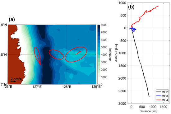
Figure 2.
(a) Time-mean velocity vectors and principal ellipses and (b) progressive vector diagram (PVD) of 48 h low-pass filtered near-bottom currents, measured by three current meters launched approximately 50 m above the seafloor. The semi-major and semi-minor axes of the principal ellipses in (a) represent the standard deviations of speeds along each respective axis.
Figure 3 displays the time series of the observed velocity (black) and 48 h low-pass-filtered velocity (red) in MP2. The southward DWBC is confirmed from the mean negative value of (−4 cm/s), of which the absolute value is four times larger than that of (1 cm/s). The reason of the southward flow direction speculates that the DWBC is influenced by the meridionally extending bottom topography of the Philippine Trench. For most of the observation period, the currents headed southward, except for June 2018 and September 2018, February 2019, and May–June 2019. The DWBC shows alternative occurrences of northward and southward flow such as the northward anomaly in May–July 2019 and southward anomaly during the period November 2017–May 2018. The standard deviation of the low-pass-filtered , which has a value of 3.1 cm/s, is larger than that of the low-pass filtered , which has a value of 1.2 cm/s. Therefore, our observation at MP2 provides evidence of a semi-permanent southward DWBC in the deep western boundary of the Philippine Trench, dominated by variability in the meridional direction.
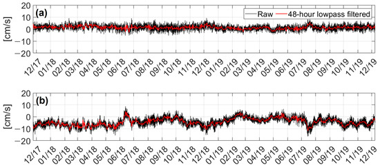
Figure 3.
Time series of observed (a) zonal and (b) meridional velocities at MP2 from 23 November 2017 to 8 December 2019. Raw velocities (black) are superimposed with 48 h low-pass filtered velocities (red).
3.2. Comparison between Observation and GLORYS12V1 Simulation
Figure 4 compares the time series of the velocity vector from the observation and the GLORYS12V1 simulation. The velocities shown in Figure 4b–e were derived from the outputs of the 45th–48th layers. Both the observed and simulated currents flow southward, indicating that GLORYS12V1 reproduced the DWBC similarly to the observed DWBC. In the 45th–48th layers, the standard deviations of (7.2, 8.0, 10.1, and 7.0 cm/s) are larger than those of (1.9, 3.6, 1.8, and 1.1 cm/s). The R values of the north–southward component are statistically significant, with values larger than 0.7 in all four layers (Figure 4b–e), verifying that GLORYS12V1 simulates the variability of the DWBC well. The reason for the high reproducibility of the GLORYS12V1 is speculated due to the data-assimilation using in situ hydrographical data obtained from ARGO floats and CTD measurements and an appropriate assimilation scheme. Previous studies reported that the reproducibility of the GLORYS12V1 on currents at intermediate and deep layers. Azminuddin et al. [25] confirmed that GLORYS12V1 could reproduce the MC and Mindanao Undercurrent (MUC), agreeing with in situ acoustic Doppler current profile measurements. Artana et al. [26] exhibited that the deep circulation pattern in the Drake Passage simulated by the GLORYS12V1 agreed well with the near-bottom currents obtained by the CPIES measurement. Among the four layers, the R value in the meridional direction has a maximum value at the 46th layer, which can be inferred to be a result of lesser distortion of the velocity fields caused by the bottom topography. Therefore, in this study, the velocity of the 46th layer (3992 m) is used for the further analysis of the DWBC variability.
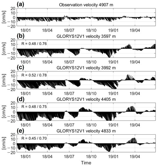
Figure 4.
Time series of velocity vectors from (a) observation at 4907 m and (b–e) simulation (GLORYS12V1) at a grid point nearest to MP2 at 4 layers (3597, 3992, 4405, and 4833 m). The two numbers included in each plot represent the correlation coefficients (R) of the zonal and meridional components between the observed and simulated velocities.
3.3. Seasonal Variability of DWBC
Before analyzing the variability, we investigate the horizontal distribution and vertical structure of the DWBC using the GLORYS12V1 outputs. The DWBC has a width of approximately 55 km at 8° N and flows southward with a mean speed of over 4 cm/s along the Philippine Trench, as shown in Figure 5a. An anticyclonic eddy, confined to a relatively flat bottom, is found in the area between 10°–13° N and 125.5°–128.5° E. The DWBC, which runs below the MC and MUC, has a vertical structure that expands from approximately 1500 m to the bottom at 8° N (Figure 5b).
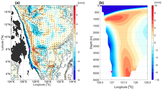
Figure 5.
(a) Velocity field of the temporally averaged velocity of GLORYS12V1 at 3992 m. The color shading indicates the mean along-slope current (), obtained through principal axis analysis. A positive value means a northward current. Gray contours represent isobaths (4000–6000 m with 500 m intervals) for the GLORYS12V1 model. (b) Longitude-depth plot of temporally averaged meridional velocity across the 8° N line. Color shading illustrates temporally averaged meridional velocity with 1 cm/s intervals. Magenta points in both plots indicate the location of the MP2 site.
To examine the seasonal variability of the DWBC and its horizontal distribution in the deep Philippine Basin, EOF analysis is applied to at 3992 m. The first-mode EOF reveals that the most dominant variability is concentrated at the western boundary where the DWBC is located, and the variance of the first mode occupies 12.9% of the total variability (Figure 6a). The first-mode PC time series (PC1) is dominated by seasonal variability (Figure 6b,d). In the variance-preserving power spectral density (PSD), the highest peak value is distributed in the seasonal band, and there are also significant peak values in the semi-annual and intraseasonal bands (Figure 6d). The monthly climatology of PC1 has a maximum in August and a minimum in December, indicating that the southward DWBC has seasonal variability that becomes stronger in winter and weaker in summer (Figure 6c). In addition to the seasonal variability of the DWBC, another seasonal variability, whose phase is opposite to that of the DWBC, is distributed adjacent to the eastern side of the DWBC. This indicates that the anticyclonic eddy identified in Figure 5a has an anticyclonic anomaly in summer and a cyclonic anomaly in winter. This result suggests a close relationship between the DWBC and topography-trapped anticyclonic eddy in terms of seasonal variability.
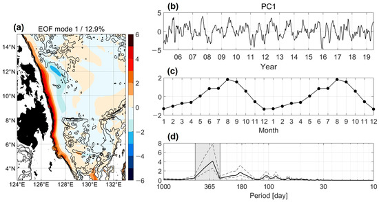
Figure 6.
(a) The first-mode empirical orthogonal function (EOF) and (b) its principal component time series (PC1) for along-slope current (), (c) climatological monthly mean of PC1, and (d) variance-preserving power spectral density (PSD) of PC1. The black contours in (a) represent the 4000–6000 m isobaths for the GLORYS12V1 model. The gray dashed lines in (d) denote the 95% confidence interval of power spectra.
From the second to fifth modes of EOFs for are distributed in the region of DWBC as well as the eastern region of DWBC (Figures S1–S4). Their PC time series are dominated by intraseasonal variability, whose power spectra are distributed in a broad period of 30–100 days. It seems that the higher-mode EOFs describes the intraseasonal variability of DWBC, which is related to the westward-propagating deep eddies originating from the eastern region of the DWBC.
Since further analyses utilize the first-mode EOF to reveal the reason for seasonal variability, it should be confirmed that the first-mode EOF reasonably represents the seasonal variability of DWBC. For this, the which is reconstructed using the result of the first-mode EOF, is compared with , and used for the EOF analysis (Figure S5). At the grid nearest to the MP2 location, the agrees well with the in terms of the seasonal variability despite tiny discrepancies coming from intraseasonal variabilities. The regression coefficient has a value of 1 with a 95% confidence interval of 0.98–1.02. Additionally, when the EOF analysis is carried out with a narrow spatial domain to include only the DWBC, its first-mode EOF occupies approximately 35.2% of the total variance and its PC time series (not shown) is the same with PC1 shown in Figure 6b. These prove that the first-mode EOF well represents the seasonal variability of DWBC.
3.4. Seasonal Variabilities of NECBL and Upper Pycnocline
The 130-day low-pass-filtered NECBL (red) oscillates in the meridional direction with a mean latitude of approximately 14° N (Figure 7a). The calculated NECBL is similar to those of Qu and Lukas [10] and Qiu and Chen [9] in terms of seasonal and interannual variabilities. However, the mean NECBL (~14° N) at 150 m depth in this study differs from those in previous studies because the NECBL has a northward bias as the depth increases [10]. Among the variabilities in the NECBL, the most dominant variability under a year is seasonal variability (Figure 7b,c). In the monthly climatology of the NECBL, seasonal variability shows southernmost migration in July and northernmost migration in October and November, which correspond to the anti-phase compared to the seasonal variability of the DWBC. Consequently, the variance-preserving power spectra of the NECBL shows a dominant peak in the seasonal band.
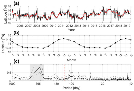
Figure 7.
(a) Time series of the North Equatorial Current bifurcation latitude (NECBL). Daily NECBL derived from GLORYS12V1 (black) is superimposed by a 130-day low-pass-filtered NECBL (red). (b) Climatological monthly mean of low-pass-filtered NECBL. (c) Variance-preserving power spectral density (PSD) of NECBL. The red dashed line denotes the cutoff frequency of 130 days, which is used for low-pass filtering in (a). The gray shaded area represents the seasonal band (290–500 days) used for bandpass filtering. The gray dashed lines indicate the 95% confidence interval of the power spectra.
To investigate the relationship between the NECBL and DWBC, coherence analysis is applied to the NECBL and PC1 of , which are dominated by seasonal variability. In the coherence analysis, the sign of the NECBL is reversed to avoid complicated explanations, owing to its anti-phase seasonality to the DWBC. The resulting coherence shows a statistically significant peak value (>0.9) in the seasonal band, suggesting a significant relationship between the two time series. Since the coherence phase expands in the range of 0°–360°, a coherence phase of 1° in the seasonal band can be regarded as a 1-day phase difference between the two seasonal variabilities. Therefore, the coherence phase of −75° in the seasonal band indicates that the seasonal variability of the NECBL leads to the seasonal variability of the DWBC by approximately 75 days (Figure 8b).
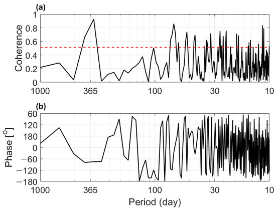
Figure 8.
(a) Coherence and (b) coherence phase between the North Equatorial Current bifurcation latitude (NECBL) and the first-mode empirical orthogonal function (EOF) principal component time series of the along-slope current (PC1). The red dashed line in (a) represents the 95% confidence level. A negative coherence phase signifies that the NECBL leads the PC1 of the along-slope current.
In the northwestern Pacific, the seasonal displacement of the pycnocline, which accompanies the seasonal variability of the NECBL, is confined to the boundary between the upper and lower pycnoclines. Figure 9 shows the seasonal variation in the upper pycnocline depth in 2012, which is one of the years showing the energetic seasonal variability of the DWBC. Since the PC1 of 2012 shows relatively weak semi-annual and intraseasonal variabilities (Figure 6b), it was selected as an example to show the distinct seasonal variability in the upper pycnocline depth. Overall, the upper pycnocline gradually thickens as latitude increased. During the summer (15 June 2012), the upper pycnocline depth in the region where the deep anticyclonic eddy exists is deepest with the southward migration of the NECBL (Figure 9b). During winter (3 January 2012), when the NECBL moves northward, the upper pycnocline depth becomes shallower in the deep anticyclonic eddy region (Figure 9d). Seasonal variation in the upper pycnocline depth is evident in the region north of 10° N, where the seasonal variation of the NECBL typically occurs. In particular, there is a notable displacement of the upper pycnocline depth in the region of 11°–13° N and 125°–128° E, where the deep anticyclonic eddy is trapped by topography (Figure 5 and Figure 9).
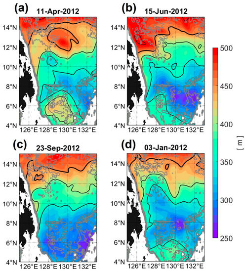
Figure 9.
Maps of upper pycnocline depth on (a) 11 April 2012, (b) 15 June 2012, (c) 23 September 2012, and (d) 3 January 2012, respectively. Black contours represent the upper pycnocline depth (350–500 m) with 50 m intervals. The thick black contour corresponds to a 450 m upper pycnocline depth near the North Equatorial Current bifurcation latitude (NECBL). Upper pycnocline depths are mapped in areas where the bottom depth is greater than 3992 m. Gray contours depict isobaths (4000–6000 m) with 500 m intervals.
3.5. Physical Processes Inducing the Seasonal Variability of DWBC
To investigate the feature of the deep anticyclonic eddy trapped by the topography, we calculated the EKE using and . The most intensive EKE is distributed along the western boundary of the Philippine Trench, which confirms the dominance of the DWBC variability (Figure 10). Except for the DWBC region, the EKE is also concentrated on flat terrain at 10°–13° N. Since the first-mode EOF of , used for and reconstruction, has predominant seasonal variability (Figure 6b), the concentration of EKE indicates the existence of a deep anticyclonic eddy identified in Figure 5a, which varies with the seasonal period (Figure 10).
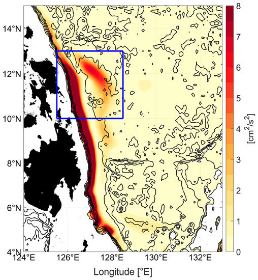
Figure 10.
Map of the eddy kinetic energy (EKE) calculated using and reconstructed from the first-mode principal component time series of along-slope current (PC1). Black contours represent bathymetry (4000–6000 m) in GLORYS12V1 with 500 m contour intervals.
Spatial averaging of the upper pycnocline depth is carried out within the blue rectangle in Figure 10, and the statistical relationship with the NECBL is investigated by applying coherence analysis (Figure 11). In the coherence analysis, the sign of the NECBL is reversed, with a positive anomaly in summer. The spatially averaged upper pycnocline depth exhibits seasonal variability and other higher-frequency variabilities (Figure 11a,c). In the seasonal variation of the spatially averaged upper pycnocline depth, the upper pycnocline depth is deepest in August and shallowest in January and February (Figure 11b). The average range of seasonal variability is approximately 27 m, comparable to the seasonally varying upper pycnocline depth of ~30 m derived from the numerical simulation results by Chen and Wu [12]. In the seasonal band, the coherence between the spatially averaged upper pycnocline depth and the NECBL is 0.88, which exceeds the 95% significance level (Figure 11d). The coherence phase of approximately −50° in the seasonal band indicates that the seasonal variability of the upper pycnocline depth follows the seasonal variability of the NECBL with a ~50-day delay (Figure 11e). As the displacement of the upper pycnocline depth should be accompanied by the displacement of the deep layer, the seasonal variation of the upper pycnocline depth in Figure 9 and Figure 11 indicates the formation of a dynamic condition that creates the seasonal variation in a deep anticyclonic eddy trapped around the topography through potential vorticity conservation.
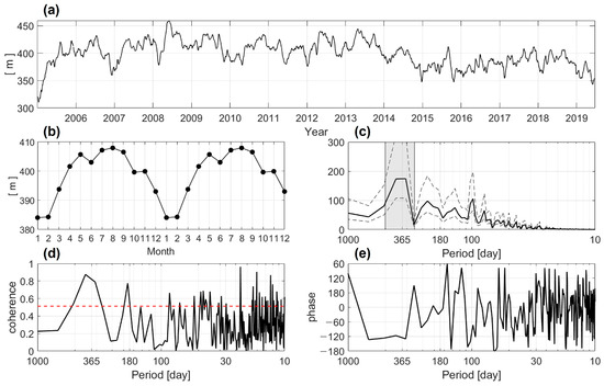
Figure 11.
(a) Time series of spatially averaged upper pycnocline depth within the area indicated by the blue box in Figure 10, and (b) its climatological monthly mean. The variance-preserving power spectral density (PSD) of (a) is depicted in (c), with gray dashed lines representing the 95% confidence interval, and the gray shaded area denoting the seasonal band (290–500 days) used for bandpass filtering. (d) Coherence and (e) coherence phase between the North Equatorial Current bifurcation latitude (NECBL) and the spatially averaged upper pycnocline depth. The red dashed line indicates the 95% confidence level (0.51). A negative phase signifies that the NECBL leads the upper pycnocline depth.
Figure 12 shows maps of and for each season in 2012, with selected dates consistent with those in Figure 9. A deep anticyclonic eddy confined to the topography changes seasonally in the interior of 10°–13° N and 125.5°–128.5° E. In summer (15 June 2012), when the upper pycnocline is deepest, the deep anticyclonic eddy is strongest among all seasons. In winter (3 January 2012), when the upper pycnocline depth is shallowest, the deep anticyclonic eddy is weakest and reduces in size. In spring (11 April 2012) and autumn (23 September 2012), the deep anticyclonic eddy has a medium intensity between summer and winter. The seasonal variability of the deep anticyclonic eddy agrees with the expected variability, which can be induced by the seasonal variability in the upper pycnocline depth shown in Figure 9 and Figure 11 through potential vorticity conservation. The western side of the deep anticyclonic eddy, which exhibits strong seasonal variability, can affect the adjacent DWBC to produce seasonality. In summer, a strong and expanded deep anticyclonic eddy blocks the passage of the southward DWBC and causes the current to flow northward (Figure 12b). Conversely, with the weakened deep anticyclonic eddy, the DWBC flows southward, which is its mean direction (Figure 12d). These results strongly suggest that the seasonal variability of the DWBC is induced by the deep anticyclonic eddy, which is affected by the seasonal variability of the upper pycnocline depth.
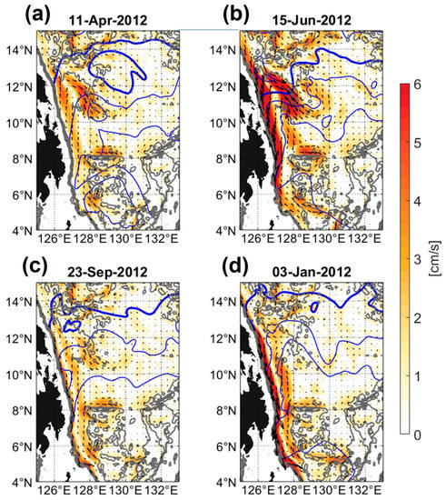
Figure 12.
Maps of the reconstructed velocity field (, ) derived from the 46th layer of GLORYS12V1. Each map displays the and fields on (a) 11 April 2012, (b) 15 June 2012, (c) 23 September 2012, and (d) 3 January 2012, respectively. Blue lines in each map represent the upper pycnocline depth (350–500 m), while the thick blue contour corresponds to a 450 m upper pycnocline depth near the North Equatorial Current bifurcation latitude (NECBL). Gray contours depict isobaths (4000–6000 m) with 500 m intervals.
To examine whether the displacement of the upper pycnocline depth is the source of the seasonal variability of the deep anticyclonic eddy, a coherence analysis is conducted with the upper pycnocline depth and relative vorticity () of the deep anticyclonic eddy. For coherence analysis, the upper pycnocline depth and are spatially averaged over the area of the blue rectangle in Figure 10. Reversed-sign is used in coherence analysis for a simple explanation in the coherence phase. Spatially averaged exhibits evident seasonal variability with a negative anomaly in summer and a positive anomaly in winter, consistent with the seasonal variability of the deep anticyclonic eddy (Figure 13a). The monthly climatology of shows negative and positive peaks in August and December, respectively, and hence, the most intensive spectra are distributed in the seasonal band (Figure 13b,c). The magnitude of coherence between the spatially averaged upper pycnocline depth and in the seasonal band has a significant value of 0.81, exceeding the 95% confidence level (Figure 13d). The coherence phase in the seasonal band is approximately −30°, representing that the seasonal variability of the upper pycnocline depth is followed by the seasonal variability of the deep anticyclonic eddy by approximately 30 days (Figure 13e). These results confirm that the seasonal variability of a deep anticyclonic eddy trapped by the topography shown in Figure 5 and Figure 12 is caused by the seasonal displacement of the deep layer thickness accompanied by the seasonal variability of the upper pycnocline depth.
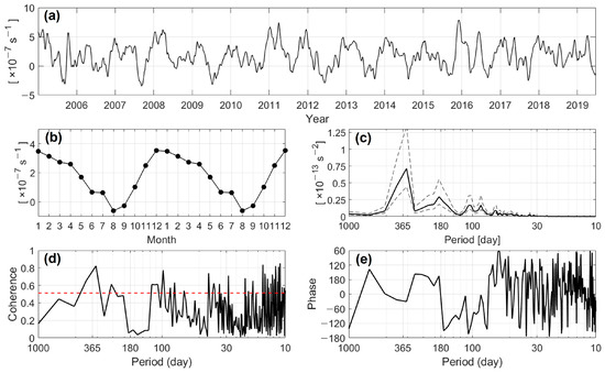
Figure 13.
(a) Time series of spatially averaged relative vorticity () within the area indicated by the blue box in Figure 10, and (b) their climatological monthly mean. The variance-preserving power spectral density (PSD) of (a) is depicted in (c), with gray dashed lines representing the 95% confidence interval. (d) The coherence and (e) coherence phase between the upper pycnocline depth and the spatially averaged . A negative phase signifies that the upper pycnocline depth leads . The red dashed line indicates the 95% confidence level.
The seasonal variations in the NECBL, upper pycnocline depth, and DWBC are compared to each other to investigate the relationships and order of occurrence (Figure 14). The amplitudes of the three variables show similar tendencies, gradually increasing in the beginning and end of the study period and decreasing in the middle of the study period (Figure 14a). Overall, the seasonal variations occurred in the order of NECBL, upper pycnocline depth, and . Although the amplitudes of the NECBL and upper pycnocline depth decrease during the period 2010–2011, the DWBC shows a small decrease in amplitude, and its peak in summer occurs before the thickening of the upper pycnocline. This implies that interannual variability can be induced by the enhancement of the Western Pacific Warm Pool owing to the extremely strong La Niña events during the period 2010–2011 [27]; the specific processes, however, are not investigated in this study. In Figure 14b, the seasonal variation of the NECBL leads to the upper pycnocline depth and by approximately 2 and 3 months, respectively, similarly to the coherence phases in Figure 8b and Figure 11e. The reasons for phase lag are demonstrated in Section 4.
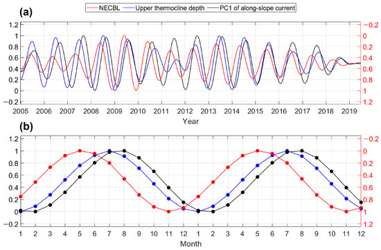
Figure 14.
(a) Normalized time series of North Equatorial Current bifurcation latitude (NECBL) (red), spatially averaged upper pycnocline depth within the blue box of Figure 9 (blue), and the first-mode empirical orthogonal function (EOF) principal component time series (PC1) of the along-slope current (black). (b) Normalized monthly climatology of the three variables presented in (a). In both plots, all variables were subjected to bandpass filtering with a cutoff band of 290–500 days. Note that the NECBL is displayed using an inverted y axis. The bandpass filtering used a cutoff of 290–500 days indicated by gray shading in Figure 6d.
4. Discussion
The intraseasonally varying signals make hard to identify a seasonal variability in the observation (Figure 4a). Therefore, the velocity ( and ) derived from the GLORYS12V1 and and reconstructed from the first- and higher-mode EOF results are compared with the observation to distinguish the seasonally and intraseasonally varying signals. Two exceptions—southward and northward flows in July–August 2018 and February 2019—break away from the seasonal variation (Figure 15a). The southward flow in July–August 2018 is also involved in both timeseries of and and the first-mode-reconstructed and (Figure 15b,c). During the same period, the spatially averaged upper pycnocline depth within 10°–13° N and 125.5°–128.5° E shows a ~20 m lower value than that in both May 2018 and September 2018. These results suggest that the southward flow of DWBC corresponds to an intraseasonal variability caused by the weakening of the deep anticyclonic eddy forced by the shrinking of the upper pycnocline. On the other hand, Figure 15c,d display that the northward flow in early March 2019, is involved not in the first-mode EOF but in the first-to-fifth-mode EOF, which occupies 38.2% of total variance (the percentage increases to 72.3% when the narrow band was adopted to only include the DWBC). The northward flow becomes stronger when the first–tenth-mode EOFs are used for velocity reconstruction. The northward flow is possibly caused by the intraseasonal variability explained by the higher-mode EOFs, the reason for which was presumed as an impact of westward-propagating deep eddies (Figures S1–S4). The two exceptions are also involved in the observation, albeit with small phase differences (Figure 15a). Therefore, it can be inferred that the two exceptions describe the intraseasonal variabilities caused by the upper pycnocline displacement and deep eddies. Except for the northward flow in February 2019, the observation agrees well with the first-mode EOF, which is dominated by evident seasonal variability (Figure 6). This suggests that the observed DWBC presents the seasonal variability—northward and southward flow in summer and winter, respectively.
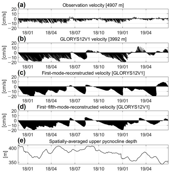
Figure 15.
Time series of velocity vectors from (a) near-bottom current measurement at MP2, (b) and derived from GLORYS12V1, (c,d) and reconstructed using the first-mode- and first–fifth-EOFs, and (e) an upper pycnocline depth spatially averaged within the area shown in Figure 10. Please note that the , , , and in (b–d) are extracted from the grid nearest to the MP2 location.
Based on the similarity of spatial distribution and significant coherence (>0.8) between the upper pycnocline depth and the relative vorticity of deep anticyclonic eddy (Figure 9, Figure 12 and Figure 13), it was suggested that the seasonal variations in the NECBL and upper pycnocline depth induce seasonal variability in the DWBC. However, the magnitude (~27 m) of the upper pycnocline depth change shown in Figure 14b needs to be quantitatively verified for its capability to produce seasonal variation in deep anticyclonic eddy through potential vorticity conservation. To verify this, the expected range of relative vorticity change induced by the 27 m vertical displacement of the upper pycnocline is calculated using a bulk formula and compared to the excursion of the relative vorticity change in Figure 13b. It was hypothesized that the region of the deep eddy trapped by the topography has a two-layer structure divided by the upper pycnocline depth, and that the change of the deep eddy is caused by the potential vorticity conservation equation, . In this equation, (2.9 × 10⁻⁵) is the local inertial frequency of 11.5° N, (3.5 × 10⁻⁷) is the winter maximum of shown in Figure 13b, and (−27 m) is the vertical displacement of the lower layer in the summer case, as determined from the monthly climatology in Figure 14b. is the thickness of the lower layer in winter, which was estimated to be 5100 m, derived from the difference between the mean depth of the deep anticyclonic region and the approximate upper pycnocline depth in winter (Figure 1 and Figure 11b). The above equation can be reduced to = , since is small enough to be neglected compared to . The expected , indicating an expected range of for the seasonal variability, is approximately −1.5 × 10⁻⁷ and its absolute values correspond to approximately 37% of a range (4.1 × 10⁻⁷) in seasonality of shown in Figure 14b. When the change within the region of the deep anticyclonic eddy (10°–13° N) is considered, the expected has a value between −1.3 × 10⁻⁷ and −1.7 × 10⁻⁷, which corresponds to 32–42% of excursion of the deep anticyclonic eddy described by Figure 13b. Although a simple equation neglecting density change in the lower pycnocline is used, the calculated is comparable to the range of the monthly climatology in Figure 14b. Therefore, it can be considered that the displacement of deep layer thickness (27 m) has the capacity to induce the seasonal variability of the deep anticyclonic eddy.
The two-layer structure that relates to the vertical first-mode was hypothesized so far. Since the MUC flows below the MC, as shown in Figure 5, a three-layer structure can also be considered. The three-layer structure would vertically relate to a second-mode as well as influence the seasonal variability of deep anticyclonic eddy. However, the simple quantitative calculation, considering the vertical first-mode, explained the capacity of the upper pycnocline displacement to induce the seasonal variability in the deep anticyclonic eddy. This indicates that the adoption of the two-layer structure is sufficient to explain the seasonal variability in the DWBC layer without considering the second- or higher-mode. In the case of the vertical first-mode, the effect of the upper pycnocline should be involved in the MUC layer. However, the signals of the westward-propagating Rossby waves, which has been known to induce the seasonality of MUC [28], were shown in the MUC layer of GLORYS12V1. Thus, it seems that the impact of the upper pycnocline displacement on MUC is hidden below the seasonality induced by the westward-propagating Rossby waves.
Figure 13e shows that the seasonal variation of the upper pycnocline depth leads to the seasonal variation in the deep anticyclonic eddy by ~30 days. This phase lag is speculated as a required-time for the adjustment of a deep anticyclonic eddy to the vertical displacement of upper pycnocline. Endoh and Hibiya [16] and Endoh and Hibiya [17] noticed that the enhancements of the topography-trapped deep eddy took ~1 month, when it was forced by vertical stretching or shrinking. The phase lag of ~50 days between the NECBL and upper pycnocline depth shown in Figure 11e is presumed to be due to the impacts of Sverdrup transport and the depth dependence of seasonal variation in the NECBL. Qu and Lukas [10] noticed that the seasonal variation of NECBL in the upper layer, which was derived from Sverdrup transport field influenced by wind stress, had a lead to the seasonal variation of NECBL, considering only geostrophic current, by 5 months. Although the velocities of 150 m depth were used for the NECBL calculation, the effect of the Sverdrup transport could be still remained. Since the upper pycnocline depth is distributed between 300 and 460 m depth, the phase lag can be caused by a decrease in wind stress effect. Additionally, it was noticed that the seasonal variation of NECBL derived from the geostrophic current occurs later as depth increases with a phase lag of 1–2 months [10]. Thus, the phase lag between the NECBL and upper pycnocline depth is possibly due to the depth dependance of its seasonal variability.
Although physical processes to induce seasonal variability were suggested, unresolved issues concerning the variability of DWBC remain. The intraseasonal variabilities are exhibited in the first-mode EOF (Figure 6) and the higher-mode EOFs which are probably related to westward-propagating deep eddies (Figures S1–S4). Additionally, the NECBL and upper pycnocline depth include the intraseasonal variability (Figure 7c and Figure 11c). These mean that the intraseasonal variability of DWBC is caused by several causes such as upper pycnocline change and deep eddies. Future study considering possible causes is required to reveal specific reasons. The interannual variability in the DWBC (shown by Figure 14a), the reason for which was speculated as extremely strong La Niña events, also remains to be investigated by future works. The seasonally varying Mindanao eddy and Halmahera eddy, located at 8° N and 4° N, respectively [29,30], can possibly affect the displacement of upper pycnocline and the resulting seasonal variability in the DWBC. However, the impacts are difficult to analyze since the eddies are located over the complicated bottom-topography and a seasonal variation of , derived from the deep layer of GLORYS12V1, is weak in the region of the two eddies. Even if the DWBC spans a meridional scale of hundreds of kilometers (Figure 5a), the in situ measurements are confined to the region at 8° N. If observational data recording temporal evolutions are collected in a broader area, it can provide a chance for further understanding in the abyssal circulation system in the Philippine Sea including the DWBC.
5. Summary and Conclusions
The two-year-long in situ near-bottom current measurements at 8° N reveal a southward DWBC on the western side of the Philippine Basin. The observed southward DWBC displays the variability dominating in the meridional direction. To investigate the reason for the seasonal variability in the DWBC, we used data-assimilated global ocean reanalysis model (GLORYS12V1) outputs, which reproduced the DWBC agreeing well with observation. The EOF analysis reveals that the DWBC is dominated by seasonal variability. Further analyses of GLORYS12V1 suggested the dynamic processes inducing the seasonal variation in DWBC (Figure 16). In summer, when the NECBL moves to its southernmost, the upper pycnocline is stretched by approximately 27 m compared to that in winter with a 2-month delay, and the deep layer thickness decreases. The deep anticyclonic eddy trapped by the topography is then enhanced through potential vorticity conservation, and its western side interrupts the southward-flowing DWBC, causing the DWBC to run northward, following the southernmost NECBL with a 3-month delay (Figure 16a). In winter, the deep anticyclonic eddy weakens due to the elevated upper pycnocline depth accompanied by the northernmost migration of the NECBL. As a result, the adjacent DWBC flows southward, which is its mean direction, due to the opening of the passage (Figure 16b). A simple calculation considering the two-layer structure reveals that the upper pycnocline depth change (~27 m) can cause a seasonal variability of comparable to the seasonal variability of a deep anticyclonic eddy. It also determines that the observed DWBC includes the seasonal variability superimposed by the intraseasonally varying signals from further analyses using the results of EOF.
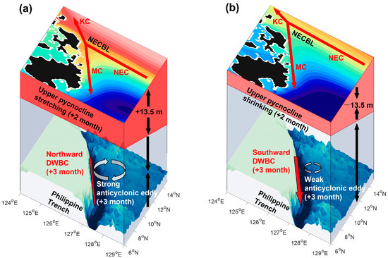
Figure 16.
Schematic diagrams illustrating the physical processes responsible for inducing the seasonal variability of the deep western boundary current (DWBC) in (a) summer and (b) winter. The periods in brackets represent the phase difference from the seasonal variability of the North Equatorial Current bifurcation latitude (NECBL).
Despite the potentially crucial role played by the DWBC in the Philippine Sea in terms of mass and heat balance and its potential to redistribute LCDW from the Southern Ocean, our understanding of its features and variability is limited due to some limitations and lack of observations. From the long-term in situ measurement and analyses on GLORSY12V1, the contentious southward direction of the DWBC was revealed. Additionally, further analyses have shown that the seasonality in the DWBC is due to a change in the vertical structure accompanying the migration of the NECBL. These results emphasize that phenomena in the near-surface layer are also a reason for seasonal variations in abyssal circulation, although it is far from the surface.
Supplementary Materials
The following supporting information can be downloaded at: https://www.mdpi.com/article/10.3390/jmse11071290/s1, Figures S1–S4: Results of higher-mode EOFs of deep along-slope current; Figure S5: Comparison between raw and reconstructed along-slope current derived from GLORYS12V1.
Author Contributions
Conceptualization, H.S. and J.-H.P.; Data curation, H.S. and J.-Y.C.; Formal analysis, H.S.; Investigation, J.-Y.C., C.J., D.-G.K., H.-S.M., J.-H.L. and J.-H.P.; Resources, X.-H.Z. and Z.-N.Z.; Writing—original draft, H.S.; Writing—review and editing, X.-H.Z., Z.-N.Z., C.J., H.-S.M., J.-H.L. and J.-H.P. All authors have read and agreed to the published version of the manuscript.
Funding
Supports for this research were provided by the “Test of long-term monitoring system installation for oceanic environmental changes caused by accelerated sea-ice melting in the Chukchi Sea (20210540)” and “Development of risk managing technology tackling ocean and fisheries crisis around Korean Peninsula by Kuroshio Current (RS-2023-00256330)”, which were funded by the Ministry of Oceans and Fisheries of Korea. This study is also sponsored by the National Natural Science Foundation of China (Grants 41920104006 and 41906024) and by the “Study on Northwestern Pacific warming and genesis and rapid intensification of typhoon (PM63400)” funded by Ministry of Oceans and Fisheries of Korea.
Institutional Review Board Statement
Not applicable.
Informed Consent Statement
Not applicable.
Data Availability Statement
The observational data presented in this study are available upon request from the corresponding author. The GLOYRS12V1 presented in this study is a publicly available dataset. The data can be found here: https://data.marine.copernicus.eu/product/GLOBAL_MULTIYEAR_PHY_001_030 (accessed on 14 January 2021).
Conflicts of Interest
The authors declare no conflict of interest.
References
- Whitworth, T., III; Warren, B.A.; Nowlin, W.D., Jr.; Rutz, S.B.; Pillsbury, R.D.; Moore, M.I. On the deep western-boundary current in the Southwest Pacific Basin. Prog. Oceanogr. 1999, 43, 1–54. [Google Scholar] [CrossRef]
- Rhein, M.; Stramma, L.; Send, U. The Atlantic Deep Western Boundary Current: Water masses and transports near the equator. J. Geophys. Res. Oceans 1995, 100, 2441–2457. [Google Scholar] [CrossRef]
- Dengler, M.; Schott, F.A.; Eden, C.; Brandt, P.; Fischer, J.; Zantopp, R.J. Break-up of the Atlantic deep western boundary current into eddies at 8° S. Nature 2004, 432, 1018–1020. [Google Scholar] [CrossRef]
- Böning, C.W.; Schott, F.A. Deep currents and the eastward salinity tongue in the equatorial Atlantic: Results from an eddy resolving, primitive equation model. J. Geophys. Res. Oceans 1993, 98, 6991–6999. [Google Scholar] [CrossRef]
- Stommel, H.; Arons, A.B. On the abyssal circulation of the world ocean-I. Stationary planetary flow patterns on a sphere. Deep Sea Res. 1960, 6, 140–154. [Google Scholar] [CrossRef]
- Zhai, F.; Gu, Y. Abyssal Circulation in the Philippine Sea. J. Ocean Univ. China 2020, 19, 249–262. [Google Scholar] [CrossRef]
- Ishizaki, H. A simulation of the abyssal circulation in the North Pacific Ocean, Part I: Flow field and comparison with observations. J. Phys. Oceanogr. 1994, 24, 1921–1939. [Google Scholar] [CrossRef]
- Wang, F.; Zhang, L.; Hu, D.; Wang, Q.; Zhai, F.; Hu, S. The vertical structure and variability of the western boundary currents east of the Philippines: Case study from in situ observations from December 2010 to August 2014. J. Oceanogr. 2017, 73, 743–758. [Google Scholar] [CrossRef]
- Qiu, B.; Chen, S. Interannual-to-decadal variability in the bifurcation of the North Equatorial Current off the Philippines. J. Phys. Oceanogr. 2010, 40, 2525–2538. [Google Scholar] [CrossRef]
- Qu, T.; Lukas, R. The bifurcation of the North Equatorial Current in the Pacific. J. Phys. Oceanogr. 2003, 33, 5–18. [Google Scholar] [CrossRef]
- Li, J.; Gan, J. On the north equatorial current spatiotemporal modes and responses in the western boundary currents. Prog. Oceanogr. 2022, 205, 102820. [Google Scholar] [CrossRef]
- Chen, Z.; Wu, L. Dynamics of the seasonal variation of the North Equatorial Current bifurcation. J. Geophys. Res. Oceans 2011, 116, C02018:1–C02018:14. [Google Scholar] [CrossRef]
- Qu, T.; Mitsudera, H.; Yamagata, T. On the western boundary currents in the Philippine Sea. J. Geophys. Res. Oceans 1998, 103, 7537–7548. [Google Scholar] [CrossRef]
- Wang, F.; Wang, Q.; Zhang, L.; Hu, D.; Hu, S.; Feng, J. Spatial distribution of the seasonal variability of the North Equatorial Current. Deep Sea Res. Part I Oceanogr. Res. Pap. 2019, 144, 63–74. [Google Scholar] [CrossRef]
- Kawase, M. Effects of a Concave Bottom Geometry on the Upwelling-Driven Circulation in an Abyssal Ocean Basin. J. Phys. Oceanogr. 1993, 23, 400–405. [Google Scholar] [CrossRef]
- Endoh, T.; Hibiya, T. Numerical simulation of the transient response of the Kuroshio leading to the large meander formation south of Japan. J. Geophys. Res. Oceans 2001, 106, 26833–26850. [Google Scholar] [CrossRef]
- Endoh, T.; Hibiya, T. Interaction between the trigger meander of the Kuroshio and the abyssal anticyclone over Koshu Seamount as seen in the reanalysis data. Geophys. Res. Lett. 2009, 36, L18604:1–L18604:7. [Google Scholar] [CrossRef]
- Jeon, C.; Park, J.H.; Kennelly, M.; Sousa, E.; Watts, D.R.; Lee, E.J.; Park, T.; Peacock, T. Advanced remote data acquisition using a Pop-Up Data Shuttle (PDS) to report data from Current- and Pressure-Recording Inverted Echo Sounders (CPIES). Front. Mar. Sci. 2021, 8, 679534. [Google Scholar] [CrossRef]
- University of Rhode Island. Inverted Echo Sounder User’s Manual; University of Rhode Island: Narragansett, RI, USA, 2015. [Google Scholar]
- Watts, D.R.; Kennelly, M.A.; Donohue, K.A.; Tracey, K.L. Four current meter models compared in strong currents in Drake Passage. J. Atmos. Ocean. Technol. 2013, 30, 2465–2477. [Google Scholar] [CrossRef][Green Version]
- Lellouche, J.M.; Greiner, E.; Galloudec, O.L.; Garric, G.; Regnier, C.; Drevillon, M.; Benkiran, M.; Testut, C.-E.; Bourdalle-Badie, R.; Gasparin, F.; et al. Recent updates to the Copernicus Marine Service global ocean monitoring and forecasting real-time 1/12° high-resolution system. Ocean Sci. 2018, 14, 1093–1126. [Google Scholar] [CrossRef]
- Fernandez, E.; Lellouche, J.M. Product User Manual for the Global Ocean Physical Reanalysis Product Gloabl_Reanalysys_PHY_001_030; Copernicus Marine Service: Toulouse, France, 2018; Available online: https://catalogue.marine.copernicus.eu/documents/PUM/CMEMS-GLO-PUM-001-030.pdf (accessed on 14 January 2021).
- Preisendorfer, R.W. Principal Component Analysis in Meteorology and Oceanography; Elsevier: Amsterdam, The Netherlands, 1988; p. 425. [Google Scholar]
- Thomson, R.E.; Emery, W.J. Data Analysis Methods in Physical Oceanography, 3rd ed.; Elsevier: Amsterdam, The Netherlands, 2014; p. 728. [Google Scholar]
- Azminuddin, F.; Lee, J.H.; Jeon, D.; Shin, C.-W.; Villanoy, C.; Lee, S.; Min, H.K.; Kim, D.K. Effect of the intensified sub-thermocline eddy on strengthening the Mindanao Undercurrent in 2019. J. Geophys. Res. Oceans 2022, 127, e2021JC017883:1–e2021JC017883:17. [Google Scholar] [CrossRef]
- Artana, C.; Ferrari, R.; Bricaud, C.; Lellouche, J.M.; Garric, G.; Sennéchael, N.; Lee, J.H.; Park, Y.H. Twenty-five years of Mercator ocean reanalysis GLORYS12 at Drake Passage: Velocity assessment and total volume transport. Adv. Space Res. 2021, 68, 447–466. [Google Scholar] [CrossRef]
- Kidwell, A.; Han, L.; Jo, Y.-H.; Yan, X.-H. Decadal western Pacific warm pool variability: A centroid and heat content study. Sci. Rep. 2017, 7, 13141. [Google Scholar] [CrossRef]
- Ren, Q.; Li, Y.; Wang, F.; Song, L.; Liu, C.; Zhai, F. Seasonality of the Mindanao Current/Undercurrent system. J. Geophys. Res. Oceans 2018, 123, 1105–1122. [Google Scholar] [CrossRef]
- Hui, Y.; Zhang, L.; Wang, Z.; Wang, F.; Hu, D. Interannual modulation of subthermocline eddy kinetic energy east of the Philippines. J. Geophys. Res. Oceans 2022, 127, e2022JC018452. [Google Scholar] [CrossRef]
- Wang, F.; Wang, Q.; Hu, D.; Zhai, F.; Hu, S. Seasonal variability of the Mindanao Current determined using mooring observations from 2010 to 2014. J. Oceanogr. 2016, 72, 787–799. [Google Scholar] [CrossRef]


Disclaimer/Publisher’s Note: The statements, opinions and data contained in all publications are solely those of the individual author(s) and contributor(s) and not of MDPI and/or the editor(s). MDPI and/or the editor(s) disclaim responsibility for any injury to people or property resulting from any ideas, methods, instructions or products referred to in the content. |
© 2023 by the authors. Licensee MDPI, Basel, Switzerland. This article is an open access article distributed under the terms and conditions of the Creative Commons Attribution (CC BY) license (https://creativecommons.org/licenses/by/4.0/).