Impact of Extreme Wind and Freshwater Runoff on the Salinity Patterns of a Mesotidal Coastal Lagoon

Abstract

The interaction between tide, river runoff, and wind in coastal lagoons induces complex salinity gradients, which are remarkable when the meteorological forcing is exacerbated. This work aims to characterize the salinity structure under extreme freshwater and wind events in the Ria de Aveiro coastal lagoon (Portugal). The Delft3D model was implemented and validated in 3D mode and used to perform simulations forced with extreme freshwater and wind scenarios. Results show that forcing conditions determine salinity stratification intensity and location. Generally, stratification increases as the freshwater increases, while the salinity intrusion moves downstream. Extreme wind tends to destroy stratification but fails to promote full-depth mixing, which is also dependent on the wind direction, as shown for the Espinheiro channel. The salinity intrusion is also impacted by wind events, being NW storms responsible for an upstream salt transport along the Mira channel and a downstream transport along the Espinheiro channel, and SW storms for an upstream displacement of the salinity intrusion along the São Jacinto channel. Finally, it is observed that the advection of a freshwater plume from the Vouga River into the middle of the São Jacinto channel under high freshwater scenarios causes an unusual local salinity pattern. This plume can either be pushed upstream or prevented from entering the channel, depending on the wind direction.

1. Introduction

Coastal lagoons are land–sea interface water bodies that experience a complex interaction between tide, river runoff, wind stress, heat, and precipitation-evaporation balances [1,2,3]. The interaction between tides and freshwater runoff is the main mechanism governing coastal lagoon salinity patterns, being responsible for the development of horizontal and vertical density gradients, which are more pronounced during neap tides and are attenuated during spring tides. However, the role of wind stress in mixing and transport processes should not be neglected [1].

The impact of freshwater runoff, as one of the main forcing factors governing the salinity patterns in coastal lagoons, has been widely studied for several coastal lagoons worldwide. Examples include Pearl Estuary, where freshwater runoff during the wet season is responsible for the establishment of a two-layer circulation, with oceanic water flowing landward in the bottom layer and freshwater flowing seaward at the surface layer [4]. Xu et al. [5] found that Chesapeake Bay’s circulation is dominated by freshwater runoff during high river flow conditions, but wind and tides can play an important role during dry conditions, while Okpeitcha et al. [6] found that Nokoué lagoon becomes completely filled with freshwater during the wet season and develops strong vertical salinity stratification at the beginning of the dry season.

The role of wind stress on the circulation patterns and horizontal and vertical salinity gradients was also widely studied in coastal lagoons worldwide. One of the most studied examples is the Patos lagoon, where the circulation is mainly wind-driven during low freshwater flow, with landward and seaward flows developing from SW and NE winds, and freshwater-driven during high discharge events [7,8,9]. Northward and southward winds are responsible for piling up freshwater on the north and south sides of the Coos estuary, respectively [10]. The wind can also be responsible for an upstream/downstream movement of the salinity intrusion and for destroying a typical two-layer circulation, as shown for the Klaipeda Strait [11].

Although wind stress usually acts as a mixer of the water column [1], opposite along-estuary winds can impact the vertical structure of the water column differently, as it happens on the Chesapeake Bay, where up-estuary winds are more effective in reducing stratification than down-estuary winds [5], and on the York River Estuary, where down-estuary winds increase stratification while up-estuary winds decrease stratification [12].

As previous studies show, wind and freshwater play a dominant role in micro-tidal estuaries and coastal lagoons. This is the same case for tidal influence, which is dependent not only on the tidal range, but also on the size and morphology of the coastal lagoon [1,3], artificial constraints, and geomorphological modifications [13,14,15,16]. Therefore, even tidally dominated estuaries and coastal lagoons can sometimes exhibit wind and freshwater-driven transport of properties [17,18,19,20]. Those impacts can be exacerbated during extreme wind events [19,21], which are often associated with high freshwater runoff events [20,22].

One example of a coastal lagoon that shows distinct dynamics depending on the balance between forcing factors is the Ria de Aveiro, a tidally dominated coastal lagoon on the Northwest coast of Portugal. Some studies were performed to understand the Ria de Aveiro lagoon dynamics under high-flow discharge conditions. Major findings pointed out that, although Ria de Aveiro may be generally classified as a well-mixed lagoon, some channels can present stratification during high freshwater discharge events, as well as a downstream displacement of the saline intrusion [23,24,25]. Moreover, Dias [23] found that wind can contribute to the establishment of local circulation patterns, mainly in shallow areas and wide channels, but its influence may not be strong enough to destroy stratification. Nonetheless, it is noteworthy that Dias [23] conducted the surveys under dry conditions during the summer. For this reason, the impact of winter season conditions on stratification patterns remains unclear. Lopes et al. [26] also found wind-induced opposite circulation patterns for NW and SE wind directions in shallow areas, as well as residual currents that are likely to act against tidal currents.

In southern Europe, extreme wind and precipitation events are associated with the occurrence of winter midlatitude cyclones [27,28]. Despite such systems usually affecting northern Europe [29], there are some case studies of low-latitude deep cyclones. Examples include storms Xynthia [30], Gong [31], and Stephanie [32], which were responsible for extreme wind conditions and heavy flooding due to continuous rainfall over the western Iberian Peninsula.

In this context, the main aim of this work is to assess the circulation and vertical salinity structure of the Ria de Aveiro lagoon under extreme wind and freshwater runoff forcing. To achieve that, the hydrodynamic model Delft3D-FLOW was implemented and validated in the 3D mode for the Ria de Aveiro lagoon. The implementation of the Delft3D-FLOW numerical model in 3D mode constitutes a first-time application to the entire Ria de Aveiro lagoon. In fact, while there are several studies based on 2DH numerical implementations of the Delft3D-FLOW model for the Ria de Aveiro [16,33,34], no research has explored a 3D implementation of this model for the same estuarine system, according to our knowledge. Moreover, the methodology defined comprises the definition and simulation of several idealized scenarios, which intend to reproduce extreme wind and freshwater discharge events, and therefore were used to investigate the generation of horizontal salinity patterns and vertical stratification.

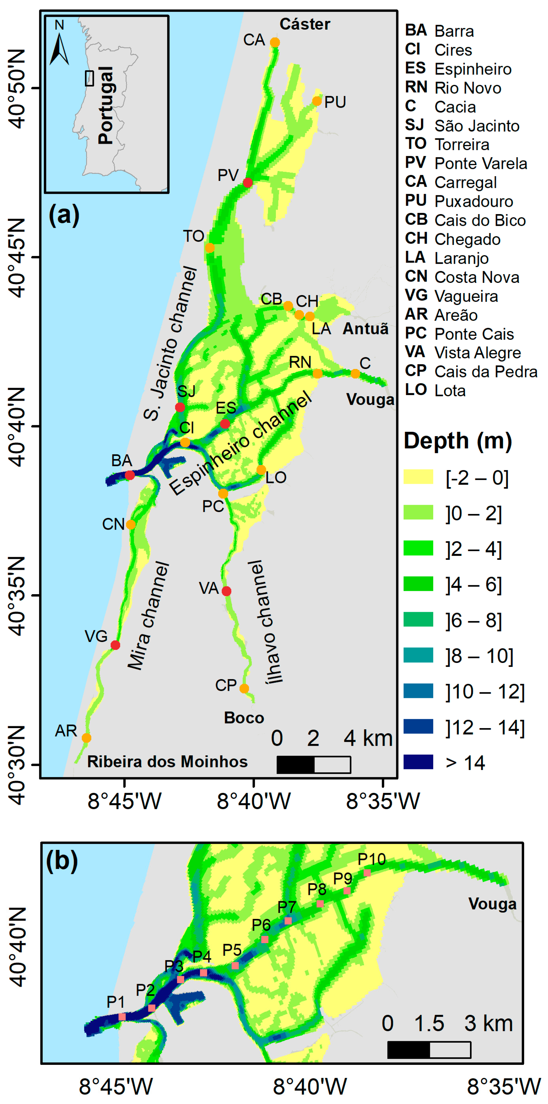
2. Study Area

The Ria de Aveiro (Figure 1) is a mesotidal coastal lagoon located on the Northwest coast of Portugal, characterized by large mudflats, salt marshes, narrow channels, and being connected with the ocean through a single, artificially fixed inlet. The lagoon is 45 km long and 10 km wide. During spring tide, it covers an area of 89.2 km² at high tide and 64.9 km² at low tide [35]. The average depth of the lagoon is 1 m, except on the main channels, where dredging operations are frequently carried out to maintain navigability conditions [36]. The lagoon has four main channels that are all connected to the lagoon’s mouth: the São Jacinto, Espinheiro, Mira, and Ílhavo channels (Figure 1).

The tides, which propagate through the inlet, are the main forcing of the circulation in Ria de Aveiro [36] and are predominantly semidiurnal, being the tidal constituents M₂ and S₂ responsible for 88% and 10% of the total tidal energy, respectively [23]. Tidal amplitude ranges between 0.46 m at neap tides and 3.52 m at spring tides [37]. The tidal wave is distorted while propagating through the lagoon, behaving as a damped progressive wave: the amplitude decreases while the phase lag increases [36]. Tidal prism was estimated between 65.8 × 10⁶ m³ and 136.7 × 10⁶ m³ at neap and spring tides, respectively [35]. However, a more recent study pointed those values at 96.9 × 10⁶ m³ and 242.2 × 10⁶ m³ [16]. In fact, the dredging operations that are frequently carried out at the main channels of the lagoon increase the depth of the cross-sectional area and, subsequently, the volume of water that flows into the system. Also, the deepening reduces the effect of bottom friction, increasing the current velocity and leading to the observed increase in the tidal prism values [38]. In addition, the ebb dominance around the lagoon’s mouth [16,38] shows the trend of the system to export sediments, which leads to a natural depth increase in this section of the lagoon. An increasing tidal influence along the last decades within the Ria de Aveiro lagoon has been reported by Araújo et al. [39], which found an average increase of M₂ amplitude by 0.245 m and an average decrease of the phase lag by 17.4° between 1987 and 2004. The changes are more remarkable at the channel’s heads, with an increase of 0.45 m for the M₂ amplitude and a decrease of 60° (~120 min), on the M₂ phase at the head of the São Jacinto channel [16], between 1987 and 2020. These tidal changes also induced an increase in the salinity intrusion, which extends further upstream than before, with annual mean salinity increases of up to 14 at the head of the São Jacinto channel [16].

The lagoon receives freshwater from five main tributaries: the Vouga, Ribeira dos Moínhos, Antuã, Boco, and Cáster (Figure 1), as well as from some superficial runoff and freshwater sources that are not well documented. Those freshwater sources correspond to a drained area of 2425 m², 302 m², 146 m², 104 m^2, and 71 m², respectively [40], and contribute to a volume of freshwater that enters the lagoon during a tidal cycle that is estimated to be 1.8 × 10⁶ m³ [41], which is considerably lower than the tidal prism.

Therefore, it can be predicted that the lagoon should generally be vertically homogeneous, although some channels can exhibit characteristics of a partially mixed estuary [36,42]. In fact, each one of the four main channels of the Ria de Aveiro presents a different morphology, tidal prism, and its own freshwater sources. Through some field measurements of salinity and water temperature, Dias [23] classified the Mira channel as a vertically homogeneous sub-estuary, while São Jacinto, Espinheiro, and Ílhavo channels were classified as partially mixed or vertically homogeneous depending on the freshwater input.

The Vouga River is the main tributary of the Ria de Aveiro lagoon, being responsible for nearly 2/3 of the total freshwater input into the lagoon [36]. Estimations of its mean freshwater flow range between 29 m³ s⁻¹ [42] and 80 m³ s⁻¹ [43], although a more recent study pointed this value to be 48 m³ s⁻¹ [25]. Due to the existence of a paper mill factory in Cacia (near station C in Figure 1) that uses freshwater in its production processes, a dam is built every year in the channel connecting the Vouga River to the Ria de Aveiro. The dam is usually built in May/June to prevent salinity intrusion during dry periods, retaining most of the freshwater upstream and allowing only a small flow to pass through [23], and it is destroyed in September/October when the river flow is strong enough. For this reason, the precipitation impact on Vouga’s freshwater input during the summer would be lower than expected if the dam did not exist, which can induce errors in freshwater input estimations during the dry season.

Measurements of freshwater flow for the Antuã, Boco, Cáster, and Ribeira dos Moínhos are practically inexistent. Consequently, it is very hard to accurately evaluate their contribution to the total freshwater input into the lagoon. Génio et al. [43] estimated mean river flows of 20 m³ s⁻¹, 10 m³ s⁻¹, 5 m³ s^−1, and 5 m³ s⁻¹ for the Antuã, Ribeira dos Moínhos, Boco, and Cáster, respectively, being their contribution small comparing with the Vouga mean freshwater flow.

The extreme river flows in Ria de Aveiro normally occur in winter and can change the salinity patterns within the lagoon [23,24,36,42]. Vicente [44] estimated peak discharge flows of 3400 m³ s⁻¹ and 4100 m³ s⁻¹ for the Vouga river, with return periods of 25, and 100 years, respectively. More recently, on the scope of the Polis Litoral Ria de Aveiro (PLRA) program [45], peak discharge flows were estimated for return periods of 2, 10, 25, 50, and 100 years for each one of the five main tributaries of the lagoon. Such peak discharge flows were based on maximum annual precipitation data for five nearby meteorological stations, which data were fit to statistical distributions and transformed into river discharge data using a hydrological model [45]. The peak discharge flows estimated by PLRA for the different return periods are shown in

Table 1. Estimated peak discharges (m³ s⁻¹) on the scope of PLRA [45] for the five main Ria de Aveiro tributaries.

Tributary	Return Period Flow (m3 s−1)
	2 Years	10 Years	25 Years	50 Years	100 Years
Vouga	374.0	745.3	1050.2	1845.1	2241.4
Cáster	69.2	108.7	136.9	199.9	227.6
Antuã	88.8	144.9	185.1	276.0	318.0
Boco	11.5	25.1	36.3	63.9	76.9
Ribeira dos Moínhos	25.7	55.5	79.7	139.2	167.3

.

The wind regime in the Ria de Aveiro region is characterized by winds blowing mainly from the North and Northwest directions, which represent more than 40% of the total wind occurrences during the year [23], and are mainly characteristic of the summer due to the coupling action of the Azores Anticyclone and the thermal depression that forms in the Iberian Peninsula [23]. In the winter, the wind regime is variable both in direction and intensity, and strong wind fluctuations are usually associated with the track of the season-characteristic deep midlatitude cyclones [28,29].

3. Methods

3.1. Model Implementation

In this work, the numerical modelling software Delft3D-FLOW was used. Delft3D-FLOW is the hydrodynamic basis for the modelling suite Delft3D, which solves the Navier–Stokes equations for an incompressible fluid, taking into account the shallow-water and the Boussinesq assumptions, and the continuity equation for vertical velocities [46]. The orthogonal, curvilinear, cartesian grid used in this work was based on a grid previously developed by Pinheiro et al. [33], but does not include the lagoon’s margins and was de-refined to minimize the computational effort. The final grid has 357 × 476 cells, with the solution computed for 32,196 nodes. The grid resolution ranges from 20 to 150 m inside the lagoon and between 100 and 400 m at the ocean boundary. A total of 10 vertical sigma layers were defined to represent the vertical salinity structure, with an increasing resolution from the bottom to the top layers.

The model bathymetry used in this work comes from different topo-bathymetric surveys performed between 1987 and 2020. The same datasets were previously used by Dias et al. [16]:

• 1987/88 by the Hydrographic Institute of the Portuguese Navy (HIPN), for the overall lagoon;
• 2011 by PLRA, for the lagoon’s main channels;
• 2011 by the Directorate-General for Territory (DGT), for the intertidal areas;
• 2020 by the University of Aveiro (UA), for the inlet channel [47];
• 2020 by the Aveiro Port Administration (APA), at a restricted area of the Mira Channel;
• 2022 by EMODnet Bathymetry Digital Terrain Model (DTM), for the continental shelf [48].

The model bathymetry was generated following Dias et al. [16]: the 1987/88 dataset covering the entire lagoon was interpolated to the numerical grid and was updated with the 2011 bathymetric survey covering the lagoon’s main channels and intertidal areas, and with the 2020 survey covering the lagoon inlet and Mira channel entrance.

The ocean boundary was forced with the amplitude and phase of the tidal constituents M₂, S₂, N₂, K₂, K₁, O₁, P₁, Q₁, MF, MM, M₄, MS₄, and MN₄, retrieved from the NAO.99b tidal prediction system [49]. The salinity and water temperature data used to build the initial and boundary conditions were retrieved from the open-source Atlantic-Iberian Biscay Irish-Ocean Reanalysis database of the Copernicus Marine Environment Monitoring Service [50]. This reanalysis has a spatial resolution of 0.083° × 0.083° and a temporal resolution of 1 day, covering 50 vertical layers between the surface and the bottom of the sea. The ocean-atmosphere boundary was forced with wind speed and direction, relative humidity, and net solar radiation retrieved from the ERA5 reanalysis database [51]. This reanalysis has a spatial resolution of 0.25° × 0.25° and a temporal resolution of 1 h. Finally, for the five main tributaries, freshwater runoff, water temperature, and salinity data were retrieved from the watershed model Soil and Water Integrated Model (SWIM) [52], calibrated for the Ria de Aveiro watershed by Stefanova et al. [53], except for the Vouga River, where freshwater inflow data collected by PLRA between March 2012 and March 2017 were used, and SWIM data were used for the simulation periods outside the aforementioned temporal range.

The bottom roughness was set following the Manning formulation, and the Manning coefficient values were adapted from those used by Lopes et al. [38] to guarantee the best match between model results and observed data, varying between 0.016 for depths higher than 10 m and 0.025 for elevations higher than 3 m. Finally, a time step of 30 s was found adequate to ensure the stability and accuracy of the model results.

3.2. Model Evaluation Methods

The model performance in reproducing tidal propagation, water currents, and the vertical and horizontal salinity patterns was assessed through a comparison between the numerical solution of the validation simulations and in situ observed data. Water level validation was performed for 18 tidal gauges located along the Ria de Aveiro lagoon (Figure 1), 12 of them with data collected in 2002 and 2003 and 13 of them with data collected between 2013 and 2019.

The 2002/03 dataset is not the best representation of the contemporary Ria de Aveiro tidal features. In fact, major dredging operations were carried out in recent years that were reflected in tidal modifications [16,38,54]. Nonetheless, this dataset was considered in the model validation because it has records for more stations than for the most recent dataset.

Hydrodynamic validation was completed with surface current velocity validation. The surface current velocity dataset is comprised of 1-day-long monitoring for 7 different stations and was retrieved in June 2019.

Surface salinity validation was performed with data collected in 7 stations along the lagoon between 2013 and 2016. Water level and salinity validation were performed for a 1-month long period, while the surface current velocity validation was performed for a 1-day long period.

The vertical dimension of the model implementation was also validated against field data; however, the lack of recent vertical profile measurement data highlighted the importance of resorting to older databases. Thus, vertical profiles of salinity performed by Vaz [24] between September 2003 and September 2004 were used to perform the vertical salinity validation of the model along the Espinheiro channel. This database presents a good spatial coverage of the Espinheiro channel, which is of uttermost importance since this channel receives freshwater from the Vouga river, the main Ria de Aveiro tributary, being, therefore, the channel where it is expected that the interaction between freshwater and ocean water can lead to the most complex vertical salinity patterns. Additionally, several vertical profiles taken in July 2011 at different points of the Ria de Aveiro lagoon under the scope of PLRA were also used to complete the model validation.

A set of simulations for a 35-day-long period (with a 5-day spin-up time, which was found adequate to ensure the stability of the numerical simulation) was performed for the water level and surface current velocity validation, while for salinity, this period was increased to 2 months, since an at least 1-month spin-up time was found necessary to stabilize the numerical results.

The model accuracy in reproducing water level, surface water velocity, and salinity was assessed through Root Mean Square Error (RMSE) [55] and predictive Skill [56] as follows:

$$\begin{array}{c}RMSE=\sqrt{\frac{1}{N}{\displaystyle {\displaystyle \sum }_{i=1}^N}{\left(M_i-O_i\right)}^2}\end{array},$$

(1)

$$Skill=1-\frac{{{\displaystyle \sum }}_{i=1}^N{\left|M_i-O_i\right|}^2}{{{\displaystyle \sum }}_{i=1}^N{\left[\left|M_i-\overline{O}\right|+\left|O_i-\overline{O}\right|\right]}^2},$$

(2)

where $N$ is the number of observations, $O_i$ is the observation values, $M_i$ is the model results and $\overline{O}$ is the mean value of the observations. The model-reproduced and observed vertical profiles of salinity were also compared through RMSE. Additionally, the water level and the surface current velocity and salinity RMSE were also compared with their local mean range (LR) through NRMSE (Normalized Root Mean Square Error):

$$NRMSE=\frac{RMSE}{LR}.$$

(3)

In each station, and for each tidal cycle, the difference between the maximum and minimum water level, surface salinity, and surface current velocity was computed, and the local mean range was defined as the mean range over all tidal cycles considered for the validation period.

3.3. Model Establishment and Scenario Definition

After the model validation, it was applied to investigate the impacts of extreme freshwater runoff and wind events in the vertical salinity structure of the Ria de Aveiro lagoon.

The definition of the extreme freshwater runoff scenarios was a challenging task. In fact, the lack of continuous monitoring of river discharge at the main lagoon tributaries leaves watershed models as the only option to reproduce river discharge properties, such as flow and water temperature. The SWIM [52] watershed model calibrated for the Ria de Aveiro by Stefanova et al. [53], and used for the model validation, is the only available numerical model that provides estimations for the aforementioned parameters for each one of the main Ria de Aveiro tributaries. However, the model’s performance is limited, as suggested by Stefanova et al. [53], which pointed out that the model significantly underestimates the high peak discharges. Moreover, Lopes [37], through peak discharge comparisons between SWIM and the Soil and Water Assessment Tool (SWAT) [57] and the estimations from PLRA [45], also found that underestimation, while SWAT validated the PLRA estimations. For this reason, despite the absence of continuous monitoring data that makes impossible to determine which one is the best database, the estimations from PLRA were imposed at the freshwater tributaries in the numerical simulations. Two different freshwater runoff scenarios were considered: a moderate flow scenario, corresponding to the 2-year return peak discharge predicted by PLRA [45], and an extreme flow scenario, corresponding to the 100-year return peak discharge. A control flow scenario was also considered for the sake of comparison, corresponding to the SWIM-predicted freshwater flow temporal series averaged between 1980 and 2010. The SWIM climatological flow considered for the control runs for each tributary is shown on

Table 2. SWIM 1980–2010 climatological flow for Ria de Aveiro tributaries.

Tributary	SWIM Mean Flow (m3 s−1)
Vouga	88.35
Antuã	7.01
Cáster	1.92
Boco	1.66
Ribeira dos Moínhos	5.61

.

The flow was imposed at the freshwater boundaries for the moderate and extreme scenarios in such a way that the flow starts linearly increasing from the climatological flow value until reaching the peak discharge in 1.5 days. After the peak flow has been reached, the flow starts decreasing linearly until returning to the climatological flow in another 1.5 days. This idealized approach is similar to that used by Lopes [37].

Regarding the wind scenarios, the ERA5 reanalysis database [51] was explored to find temporal series of mean wind speed and direction of the extreme wind events Xynthia [30], Gong [31], and Stephanie [32], in a point located at the Ria de Aveiro lagoon. Hourly time series were retrieved and analysed (Figure 2).

According to the aforementioned dataset, the 3 storms had similar intensity, with the hourly averaged wind speed peaking at about 60 km h⁻¹. However, while for the Gong and Stephanie storms, the peak wind intensity occurs in an NW wind direction, for Xynthia storms, the storm peak matches with an SW wind direction. Moreover, the duration of the storm varies greatly in each case, and the wind rotates several times during the storm, which makes it difficult to carry out a comparative analysis of the storm’s impacts on the vertical salinity structure of the Ria de Aveiro lagoon. For this reason, idealized wind scenarios based on the real characteristics of the storms were defined. The first scenario was based on storm Xynthia, but the wind direction was fixed at SW (coinciding with the wind direction at the peak intensity of the storm). The second scenario was based on storms Gong and Stephanie, with the wind direction fixed at NW, following the same approach. Moreover, in each scenario, the peak wind intensity was fixed at 60 km h⁻¹, in agreement with the real storm magnitude. A similar approach was used for freshwater runoff: the wind speed starts linearly rising from a calm scenario (no wind) until reaching the peak wind intensity in 1.5 days. After the wind reaches the maximum intensity, the wind speed starts slowing down until returning to zero-wind intensity in 1.5 days. The definition of these idealized scenarios allows us to evaluate if different wind directions have a different impact on the horizontal and vertical salinity distribution within the lagoon.

As stated above, the Ria de Aveiro lagoon is generally vertically homogeneous, except during high freshwater runoff events where stratification can develop in some channels [36,58,59]. Moreover, windstorms in Southwestern Europe are often associated with extreme rainfall events that lead to river flooding [60]. For this reason, a coupled assessment between extreme freshwater discharge (which tends to develop stratification) and extreme wind events (which tends to destroy stratification) assumes an interesting challenge. Therefore, wind scenarios were coupled with extreme freshwater runoff scenarios, and the impacts of NW and SW storms on stratification and salinity intrusion will be further assessed.

Table 3. Wind and freshwater conditions of each scenario (resume).

Scenario Resume	Wind	Freshwater Runoff
Control	No	Climatological flow
Moderate flow	No	2-year return period
Extreme flow	No	100-year return period
Control + Windstorm NW	60 km h−1 NW	Climatological flow
Moderate flow + Windstorm NW	60 km h−1 NW	2-year return period
Extreme flow + Windstorm NW	60 km h−1 NW	100-year return period
Control + Windstorm SW	60 km h−1 SW	Climatological flow
Moderate flow + Windstorm SW	60 km h−1 SW	2-year return period
Extreme flow + Windstorm SW	60 km h−1 SW	100-year return period

resumes the main characteristics of the defined scenarios.

Finally, neap and spring tide conditions were considered for the 9 scenarios (typical neap tidal range at Barra station ~1 m); however, it opted to only explore the neap tide scenarios, as will be explained in due course.

This assessment is completed through the computation of the water column stratification measurement Brunt–Väisälä buoyancy frequency as follows:

$$\mathit{N}=\sqrt{-\frac{\mathit{g}}{\mathit{\rho }}\frac{\mathcal{\partial }\mathit{\rho }\left(\mathit{z}\right)}{\mathcal{\partial }\mathit{z}}},$$

(4)

where $g$ is the gravity acceleration, $\rho$ is the water density, and $z$ is the depth (positive upward). The subsequent analysis is made under the assumption that water temperature-induced stratification in Ria de Aveiro is low, and therefore the Brunt–Väisälä frequency values are mainly driven by salinity vertical gradients. In fact, the salinity gradients have already been used as a proxy for water column stratification in a previous study of the Espinheiro channel [59], which supports the confidence in this assumption.

4. Results

4.1. Model Validation

The model accuracy in reproducing tidal propagation and surface and vertical salinity was assessed through a comparison between the model results and the in situ measured parameters. This comparison was supported by the RMSE, predictive Skill, and NRMSE calculation, as aforementioned. The results suggest a good fit between the model results and the observed water level time series (

Table 4. Estimated RMSE (m), predictive Skill, and NRMSE (%)of model-reproduced water level time series for 1 month.

Station	2002/2003			2013/2014/2019
	RMSE (m)	Skill	NRMSE (%)	RMSE (m)	Skill	NRMSE (%)
Areão	-	-	-	0.12	0.983	10
Barra	0.05	0.999	3	0.04	0.999	2
Cacia	0.25	0.964	16	-	-	-
Cais do Bico	-	-	-	0.09	0.996	4
Cais da Pedra	0.20	0.959	15	0.18	0.968	13
Carregal	0.57	0.679	48	0.13	0.990	7
Chegado	-	-	-	0.12	0.992	6
Cires	0.12	0.994	5	-	-	-
Costa Nova	0.19	0.979	12	0.08	0.997	4
Laranjo	0.10	0.995	5	-	-	-
Lota	0.08	0.997	4	-	-	-
Ponte Cais	0.08	0.997	4	-	-	-
Ponte Varela	-	-	-	0.09	0.995	5
Puxadouro	-	-	-	0.15	0.978	11
Rio Novo	-	-	-	0.13	0.992	6
Torreira	0.12	0.990	8	0.09	0.995	5
Vagueira	0.11	0.993	6	0.09	0.994	5
Vista Alegre	0.12	0.986	9	0.11	0.990	7

). The best results are achieved for the stations closest to the inlet, such as Barra, Costa Nova, Lota, Ponte Cais, and Cais do Bico, with the RMSE representing less than 5% of the local tidal range and Skill values of over 0.99. The model performance decreases upstream of the lagoon’s channels, with less accurate results being obtained for the stations located at the channel’s heads (Areão, Cacia, Cais da Pedra, Puxadouro, and Carregal), but generally, the RMSE values do not exceed 15% of the local tidal range while the Skill values maintain very close to 1. The worst fit is observed at the Carregal station for the 2002/2003 dataset, with the RMSE value representing 48% of the local tidal range and a fairly low Skill value (0.679). However, this value is not accompanied by the 2013/2014/2019 dataset, which shows a good fit between the model results and the observed data (Skill value of 0.990 and RMSE value representing only 7% of the local tidal range).

Regarding the surface current velocity (

Table 5. Estimated RMSE (m s⁻¹), predictive Skill, and NRMSE (%) of model-reproduced surface current velocity time series for 1 day.

Station	2019
	RMSE (m s−1)	Skill	NRMSE (%)
Cais da Pedra	0.077	0.502	47
Costa Nova	0.093	0.960	13
Ponte Varela	0.125	0.942	12
Rio Novo	0.229	0.599	38
Torreira	0.146	0.928	17
Vagueira	0.115	0.865	25
Vista Alegre	0.095	0.861	27

), the fit between the model results and the observed time series is lower than for the water level variable. Nevertheless, the results are generally good, with RMSE values not exceeding 25% of the local surface current velocity range and Skill values of over 0.850, except for the Cais da Pedra and Rio Novo stations, where model results are less accurate, with Skill values of 0.502 and 0.599 and RMSE values representing 47% and 38% of the local range, respectively.

The model performance in reproducing surface salinity (

Table 6. Estimated RMSE, predictive Skill, and NRMSE (%) of model-reproduced surface salinity (Sal.) time-series for 1 month.

Station	2013/2016
	RMSE	Skill	NRMSE (%)
Barra	0.79	0.809	64
Chegado	3.73	0.833	37
Costa Nova	1.06	0.678	46
Ponte Varela	4.31	0.621	59
Rio Novo	5.90	0.869	25
Vagueira	2.50	0.969	14
Vista Alegre	1.79	0.939	20

) is generally less accurate than for tidal propagation. The best results are found at Vagueira and Vista Alegre stations, with RMSE values representing 14 and 20% of the local surface salinity range, and Skill values of over 0.900, while Costa Nova, Ponte Varela, and Barra stations present the less accurate results, with RMSE exceeding 45% of the local surface salinity range and low Skill values (less than 0.7 for Costa Nova and Ponte Varela stations).

The evaluation of the performance of the model implementation developed was completed with the validation of the model results along the vertical. This assessment was supported by the comparison between model results and observed salinity vertical profiles for several stations located at the Ria de Aveiro lagoon, and on the computation of the RMSE of the model-reproduced vertical profiles (Figure 3).

The model results show that the model is generally able to reproduce the in situ observed vertical gradients. This is particularly clear from the analysis of the vertical profiles taken in the wet season, where stratification is well represented despite being fairly underestimated. Moreover, RMSE range between 0.5 and 4.1 for the vertical salinity profiles. The best results are achieved on stations close to the inlet (P1, P2, BA, ES, and SJ), with RMSE between 0.9 and 1.1, while the less accurate results are found in the upstream stations (P9, P10, and PV), with salinity RMSE ranging between 2.5 and 4.1.

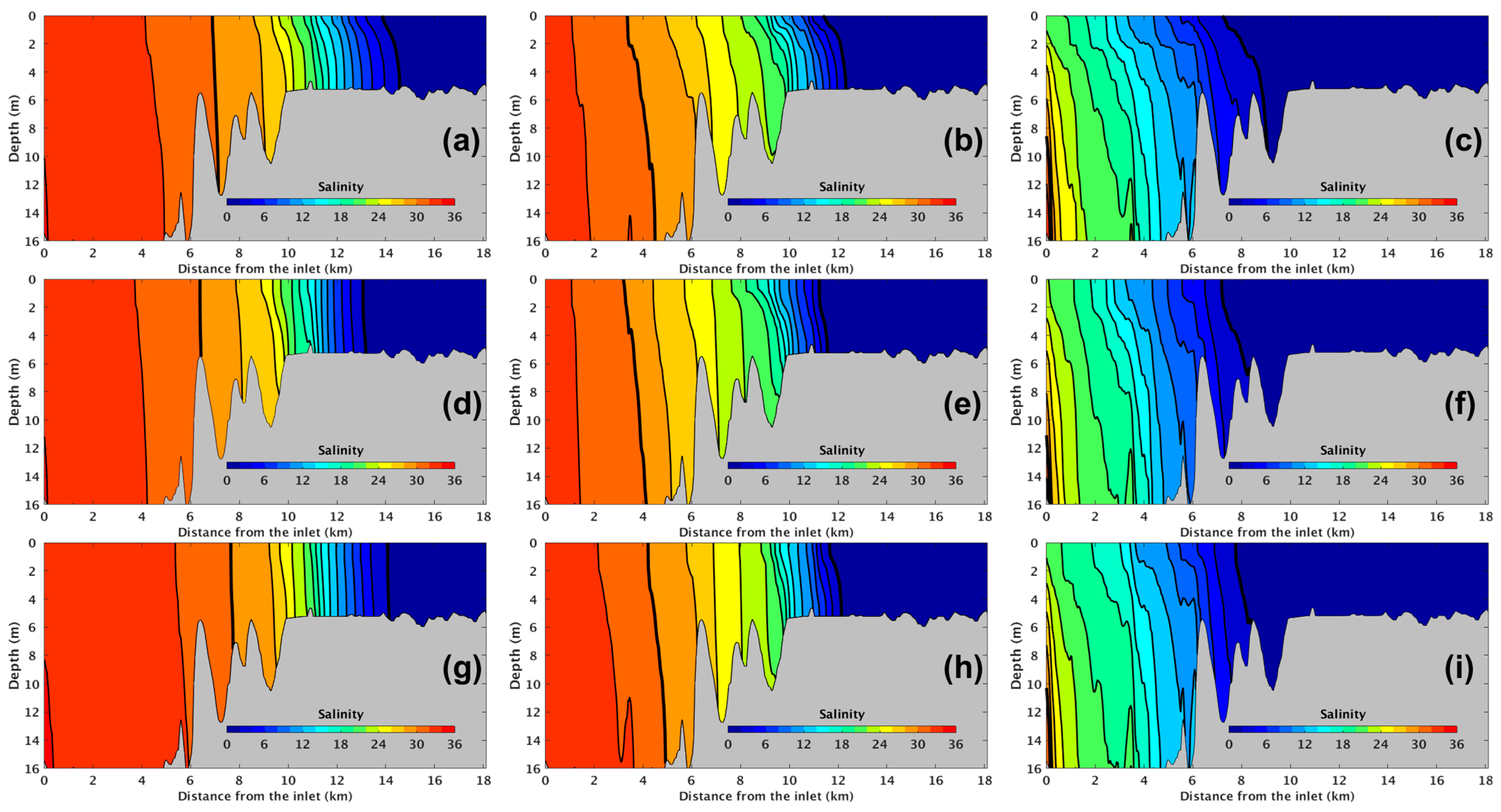
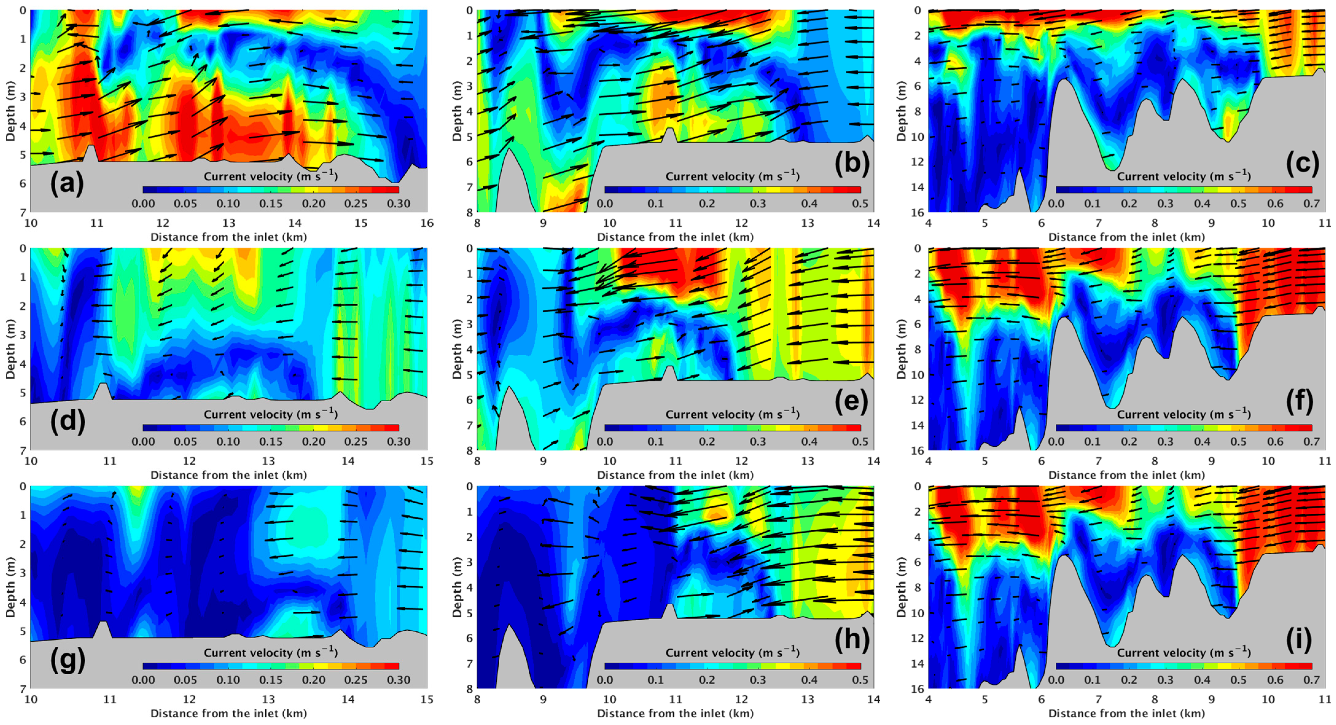
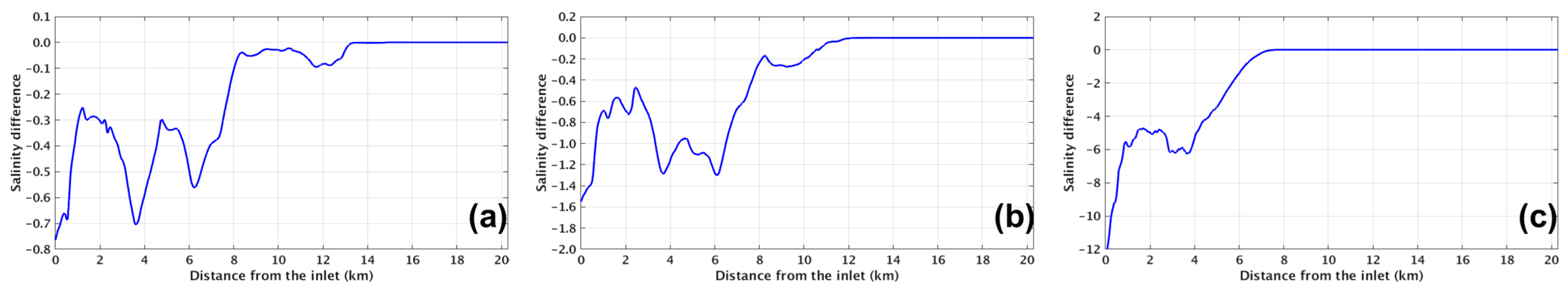
4.2. Vertical Structure of the Ria de Aveiro Main Channels

The previously validated model implementation was used to examine the effects of extreme freshwater runoff and wind events on the vertical salinity structure of the four main branches of the Ria de Aveiro lagoon. This subsection will be focused on analysing the results obtained from the numerical simulations for the different scenarios. The extension of the salinity intrusion was assessed through the position of the 2 isohaline (X₂). This metric has been first applied by Jassby et al. [61] for San Francisco Bay and is now used in several freshwater-influenced microtidal and mesotidal estuaries and coastal lagoons worldwide that refer to the extension of the salinity intrusion as a function of X₂ [62,63,64]. The salinity stratification assessment is completed by computing the Brunt–Väisälä buoyancy frequency for all scenarios.

Figure 4 and Figure 5 depict the tidally averaged longitudinal vertical salinity sections connecting the Ria de Aveiro inlet with the head of the Espinheiro channel and the along-channel salinity differences between the surface and the bottom, respectively. The presence of typical estuarine salinity gradients is a common feature that is observed in all scenarios: the highest salinity values occur at the inlet, decreasing upstream with salinity close to zero at the channel head. For the control scenarios, a transition zone between the saltier water masses and freshwater is located nearly 10–14 km upstream of the inlet. In this zone, salinity decreases abruptly upstream from nearly 26 to the 2 isohaline. Vertical salinity gradients are observable in the salinity transition zone for the no-wind control scenario (Figure 4a), with freshwater flowing close to the surface and saltier water flowing along the bottom layers of the water column. Such water masses give arise to salinity gradients of up to five between the surface and the bottom of the channel (Figure 5a), which are reduced to 4 and 2 for NW and SW storms, respectively (Figure 5d,g). For a NW storm (Figure 4d), the 2 isohaline is pushed nearly 1 km downstream than for the no-wind and SW (Figure 4g) storm scenario.

Regarding the 2-year return freshwater flow scenarios, the salinity transition zone is located 10–12 km upstream of the inlet, as the 2 isohaline is pushed 2 km downstream. Vertical salinity gradients of up to 10 and 8 (Figure 5b,e) are observable for the no-wind (Figure 4b) and NW-storm (Figure 4e) scenarios, respectively, in the transition zone and are reduced to 5 under the SW storm scenario (Figure 5h). Again, the 2-isohaline is located 1 km closer to the inlet for the NW storm scenario than for the no-wind and SW storm scenarios. Finally, for the 100-year return freshwater flow scenarios, the freshwater influence is extended even more downstream, with low salinity water reaching the inlet on the surface layers. The salinity transition zone is located between 0–8 km of the inlet, with the 2 isohaline located 6 km closer to the inlet than for the control scenarios. Vertical salinity gradients are present in the salinity transition zone for the 3 scenarios, but are more remarkable for the no-wind scenario (Figure 4c). The vertical salinity gradients are remarkable even at the inlet, contrary to what is observed for the control and 2-year return freshwater flow scenarios, with salinity differences of up to 12 between the surface and the bottom.

As referred before, the vertical salinity gradients suggest that a two-layer circulation occurs in the Espinheiro channel. Figure 6 shows the longitudinal vertical sections of current velocity and direction. The two-layer circulation, with ocean water flowing inward and freshwater flowing outward, is evidenced in the current velocity transects. This circulation is stronger under no-wind scenarios. For the control and 2-year return no-wind scenarios (Figure 6a,b), strong fluxes occur both inward in the deep layers and outward in the superficial layers, with current velocities reaching up to 0.3 and 0.5 m s⁻¹, respectively. Under 100-year return freshwater flow conditions (Figure 6c), the inward flux is stopped, and even stronger outward fluxes occur, with current velocities reaching up to 0.7 m s⁻¹ in the superficial layers. When extreme wind events are considered, the two-layer circulation is broken, especially under SW storm winds. Under 100-year return freshwater flow conditions (Figure 6f,i), strong outward fluxes with current velocities up to 0.7 m s⁻¹ still occur, and the bottom inward flux remains practically null.

Figure 7 depicts the longitudinal vertical sections of the Brunt–Väisälä frequency for the Espinheiro channel. Salinity stratification is common to all no-wind scenarios and is coincident with the aforementioned ocean water-freshwater transition areas, with maximum frequencies of 80, 100, and 70 cycles h⁻¹, respectively, for control (Figure 7a), 2-year (Figure 7b) and 100-year (Figure 7c) return freshwater flow scenarios, respectively. Under NW storm conditions, the salinity stratification is weakened and restricted to a smaller area, especially for control (Figure 7d) and 2-year return (Figure 7e) freshwater flow conditions, as the maximum frequencies of 40 and 80 cycles h⁻¹, respectively, suggest. Under SW storm conditions, salinity stratification practically disappears for the control scenario (Figure 7g) and is limited to a maximum of 50 cycles h⁻¹ for the 2-year return (Figure 7h) freshwater flow conditions. For the 100-year return scenarios, salinity stratification is restricted to the deeper sections of the channel and seems to be poorly affected by NW (Figure 7f) and SW (Figure 7i) storms, contrarily to the control and 2-year return scenarios, with Brunt–Väisälä frequencies of up to 50 cycles h⁻¹ being noticed even for storm conditions.

Figure 8 depicts the tidally averaged longitudinal vertical salinity sections connecting the Ria de Aveiro inlet with the head of the Ílhavo channel.

A common feature of all scenarios is the absence of vertical salinity gradients, as the isohalines are practically perpendicular to the surface. For the control scenarios, the transition between the 30 and the 2 isohalines occurs between 9 and 20 km upstream of the inlet, and between 4 and 18 km for the 2-year return scenarios. For the 100-year return freshwater flow scenarios, the lower depths of the Ílhavo channel become completely filled with freshwater, being the 2 isohaline located 12 km upstream of the inlet. A lower salinity surface water mass, with salinity values of nearly 5, is visible nearly 6 km upstream of the inlet. Considering the absence of vertical salinity gradients for the Ílhavo channel, regardless of the scenarios was found irrelevant to compute the salinity difference between the bottom and the surface and the salinity-derived Brunt–Väisälä frequency for this channel.

Figure 9 and Figure 10 depict the tidally averaged longitudinal vertical salinity sections connecting the Ria de Aveiro inlet with the head of the Mira channel, and the salinity differences between the bottom and the surface, respectively.

For the control freshwater flow scenarios, vertical salinity gradients are practically null, with differences between the surface and the bottom of less than 1, and the transition zone between the 30 and 2 isohaline is located between 4 and 14 km upstream of the inlet, except for the SW storm scenario (Figure 9g), where the 2 isohaline is actually 2 km closer to the inlet. Concerning the 2-year return freshwater flow scenario, the 30 and 2 isohalines are located between 3 and 11 km upstream of the inlet for the no-wind (Figure 9b) and storm (Figure 9e,h) scenarios. Small vertical salinity gradients (up to 1.5 between the surface and the bottom) are observable between 4 and 6 km upstream of the inlet for the no-wind scenario (Figure 10b). Finally, for the 100-year return freshwater flow scenario, the Mira channel is mostly filled with freshwater, being the 2 isohaline located 6 km upstream of the inlet and the 30 isohaline pushed away from the channel. Vertical salinity gradients of up to 6 are noticeable at the entrance of Mira channel (between 2 and 6 km upstream of the inlet) for the no-wind (Figure 10c), being limited to up to 3 for windstorm (Figure 10f,i) scenarios.

The highest Brunt–Väisälä frequencies (Figure 11) are observed for the no-wind scenarios, with values of up to 20, 50, and 90 cycles h⁻¹ for control (Figure 11a), 2-year (Figure 11b) and 100 years (Figure 11c) freshwater flow scenarios. Salinity stratification is restricted to a small area between 2 and 6 km upstream of the inlet for all no-wind scenarios. This stratification is destroyed during storm conditions for the control and 2-year return scenarios and is restricted to the inlet for 100-year return freshwater flow conditions.

Finally, Figure 12 and Figure 13 depict the tidally averaged longitudinal vertical salinity and the salinity differences between the surface and the bottom along the São Jacinto channel. For the control freshwater flow scenarios, the 30 isohaline is located 9–10 km upstream of the inlet, while the 2 isohaline is observed at the Cáster River inlet. High salinity values (between 26 and 30) are observed in most of the channel, with freshwater influence being restricted to the channel head, and vertical salinity gradients are very low. For a 2-year return freshwater flow scenario, the 30 isohaline is located 3–6 km upstream of the inlet for the no-wind (Figure 12b), and NW storm (Figure 12e) scenarios and 7 km for a SW storm (Figure 12h) scenario, and the freshwater influence is still restricted to the lower depths of the São Jacinto channel, with the 2 isohaline being located 26–27 km upstream the inlet. For the no-wind and SW-storm scenarios, lower salinity water masses (up to 2-salinity lower than the surrounding water masses) are observed between 12 and 15 km upstream of the inlet. This low salinity water mass is restricted to the first 2 m depth for the no-wind scenario and comprises the entire water column for the SW storm scenario, being absent from the NW storm scenario.

Perhaps the most interesting features can be observed for the 100-year return freshwater flow scenarios. For both scenarios, the 30 isohaline is located outside the lagoon, while the 2 isohaline is located 24 km upstream of the inlet. Along with the predictable salinity minimum at the Cáster River inlet, a water mass with low salinity values (between 14 and 18) is observed between 6 and 12 km upstream of the inlet, followed by a salinity maximum of 20 located by 15–21 km upstream. This atypical estuarine pattern is common to all scenarios, but is more remarkable for the no-wind (Figure 12c) and SW storm (Figure 12i) scenarios. Vertical salinity gradients of up to 8 are observed at the high salinity water mass and are practically null for the low salinity water mass (Figure 13c), whereas they are limited to up to a maximum of 4 for the storm scenarios.

Regarding the no-wind scenarios, the salinity stratification is practically null for the control freshwater scenario (Figure 14a), but is significant for the 2 (Figure 14b) and 100-year (Figure 14c) return freshwater flow scenarios, with Brunt–Väisälä frequencies reaching up to 70 and 100 cycles h⁻¹, respectively. Two zones of water column salinity stratification maxima are identified: the first one between 12 and 18 km upstream of the inlet and the second one between 21 and 24 km upstream of the inlet. Windstorm scenarios, regardless of the direction, are effective in destroying salinity stratification in the superficial layer for all scenarios, being responsible for the null vertical salinity stratification for the control and 2-year return scenarios. For the 100-year return scenarios, the wind stress only destroys salinity stratification at the upper layers since Brunt–Väisälä frequency values of up to 50 cycles h⁻¹ can still be found between 1 and 5 m deep.

Given the importance of understanding the interesting salinity patterns found for the São Jacinto channel, synoptic snapshots of the depth-averaged salinity were computed for the high tide for each scenario (Figure 15). The depth-averaged salinity fields are complemented by the depth-averaged velocity magnitude and direction fields depicted in Figure 16. The salinity fields reveal some interesting features of the São Jacinto channel that could not be observed just from the longitudinal channel section analysis. Regarding the 2-year freshwater flow scenarios, although the channel is generally filled with brackish water with a salinity of around 26 (except at the Cáster river inlet), it can be observed a plume with lower salinity values (about 12–14) coming from the Vouga and Antuã rivers, that propagates into the São Jacinto channel through its eastern side during the flooding tide. This pattern is also observed for the 100-year return scenarios, although with lower salinity values: the higher salinity plume has salinity around 18–20, and the low salinity plume is practically composed of freshwater. For both freshwater scenarios, the freshwater plume propagation into the São Jacinto channel is favoured by SW winds, advancing up to 3.5 km upstream than for the NW storm scenarios. In fact, under NW winds, the low salinity plume practically cannot progress upstream, being retained in the wider basin of the Ria de Aveiro.

Regarding the depth-averaged current velocity fields, landward fluxes occur in all scenarios, with current velocities of up to 0.6 m s⁻¹ in the deeper sections of the São Jacinto channel, and up to 0.2 m s⁻¹ in the shallower areas (between 40°44′ N and 40°46′ N), for no-wind scenarios (Figure 16a,d). Under NW storm scenarios (Figure 16b,e), while the landward flux keeps existing in the deeper section of the channel, it is practically null in the shallower areas. In opposition, under a SW storm (Figure 16c,f), the landward flux is favoured, with current velocities of up to 0.4 m s⁻¹ occurring both in the deeper sections and in the shallower areas.

5. Discussion

5.1. Model Performance Assessment

The model implementation was developed and firstly validated against water level and surface current velocity and salinity time series. The model revealed high accuracy in representing the tidal propagation within the lagoon. NRMSE values lower than 10% and predictive Skill values above 0.95 reflect a good agreement between the model results and the observed data [65], which occurs in most stations. This agreement can even be considered excellent for the stations close to the inlet, with NRMSE values representing less than 5% of the local mean tidal range [65]. The model performance decreases with the distance from the inlet, with less accurate results being obtained for the stations located at the channel’s heads. This could be due to the grid derefinement applied to minimize the computational effort, which may have led to inaccurate resolution of some narrower channels represented in the model bathymetry.

The model performance when modelling surface current velocity is not as good as when reproducing the SSE patterns. Nevertheless, RMSE represents between 10 and 30% of the local current velocity range, and predictive Skill values between 0.85 and 0.95 reveal reasonable accuracy when predicting the surface current velocity for most of the stations. However, the results are less accurate for Cais da Pedra and Rio Novo stations, with RMSE values representing 47% and 38% of the local current velocity range and low Skill (below 0.60). These stations are located in areas with very narrow channels that are probably not well resolved by the numerical grid, leading to differences between the model results and the observed data, as had been already related by Mendes et al. [66] in a previous modelling application for Ria de Aveiro. Nevertheless, it can be considered that the model implementation is able to reproduce surface current velocity during a tidal cycle.

The comparison between the model results and observed data also revealed that the model performance when predicting surface salinity patterns varies greatly along the lagoon. The best fit was achieved for Vagueira and Vista Alegre stations, with RMSE values representing less than 20% of the local surface salinity range, and reasonably high predictive Skill values (over 0.900), whereas for Barra, Costa Nova, and Ponte Varela stations, the model results are not so accurate, with RMSE values exceeding 40% of the local salinity range. Firstly, it should be noted that the salinity depends on the prescribed freshwater input. Following Stefanova et al. [53], SWIM strongly underestimates peak discharges. On the other hand, a comparison between the temporal series of freshwater inflow for the Vouga River obtained in situ under the scope of PLRA and SWIM results revealed that the watershed model strongly overestimates summer freshwater inflow. Therefore, it is possible to conclude that the SWIM freshwater inflow temporal series applied at the five main tributaries constitute a major source of errors in the efforts conducted to reproduce the salinity evolution, and, for this reason, it is advisable to exercise caution when interpreting the model results. In addition, it should be considered that Ria de Aveiro receives freshwater from several sources that are not well documented and therefore cannot be considered in the modelling efforts, as well as some superficial runoff [23], that could contribute to exacerbating the errors in reproducing the salinity evolution. Nevertheless, the model results can be considered reasonable, and the model implementation developed can be considered suitable for the representation of hydrodynamics and surface salinity patterns, ensuring a good representation of the extreme wind and freshwater effects on horizontal salinity transport.

Considering that extreme wind and freshwater conditions foment not only horizontal transport throughout the lagoon, but also important processes of mixing and stratification of the water column, it is not adequate to limit the model validation to surface data. It is needed to ensure that the model is able to reproduce the aforementioned processes properly. For this reason, the model validation was performed as well for the vertical dimension. Here, a comparison between observed vertical profiles and the model results revealed that the model is able to reproduce salinity patterns in the entire water column. Salinity RMSE values ranging between 0.5 and 4.5 are relatively small. Moreover, the model is capable of reproducing salinity stratification due to the interaction between freshwater and ocean water, although this stratification may be underestimated, especially close to the Vouga inlet. This effect was also documented by Vaz et al. [24] in their 3D modelling efforts of the Espinheiro channel using the MOHID model.

It should be noted that it was impossible to validate the model properly for the São Jacinto, Ílhavo, and Mira channels due to the lack of vertical profile measurements, which means that the results obtained should be taken carefully. Nonetheless, the good coverage of the dataset used to validate the model at the Espinheiro channel allows for a degree of confidence in the results obtained for this channel, which is, as referred before, of uttermost importance due to the relevance of the freshwater runoff at the Espinheiro channel. For this reason, the model validation for the vertical dimension can be considered successful.

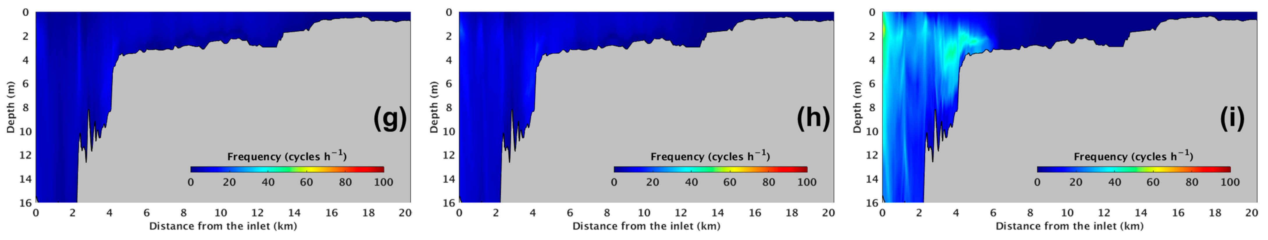
5.2. Vertical Salinity Structure of the Ria de Aveiro Main Channels

The previously validated implementation of the Delft3D-FLOW was used to examine the vertical salinity structure of the Ria de Aveiro lagoon’s four main channels: the Espinheiro, Ílhavo, Mira, and São Jacinto. This analysis was focused on studying the impact of extreme wind and freshwater runoff events on salinity patterns. The results revealed that the salinity structure of the Espinheiro channel is strongly dependent on the freshwater inflow: as the freshwater runoff increases, the freshwater influence extends towards the inlet. Moreover, a two-layer circulation is evident in this channel, in agreement with Vaz et al. [24] findings, with ocean water flowing upstream in the deep layers and outward fluxes of freshwater in the surface layers. An intermediate area with practically null velocities suggests the presence of an estuarine front in the Espinheiro channel. The estuarine front tends to get bigger and migrate outward as the freshwater runoff increases. For a 100-year return freshwater runoff, the estuarine front has approximately 10 km length, which is consistent with the extension of the salinity stratification. Strong horizontal salinity gradients are established in the distance between 8 and 14 km off the inlet for control and 2-year return freshwater flow scenarios, and can be explained by the interaction between the salty and freshwater, as well as by changes in the channel’s morphological characteristics, such as the channel narrowing and depth decreasing that occur about 9 km off the inlet, as also suggested by Vaz and Dias [59]. Contrary to what was found by Vaz and Dias [59], a freshwater runoff of 374 m³ s⁻¹ was not enough to extend the salinity stratification towards the inlet, which only happened for a 100-year freshwater flow return period; however, it should be noted that the results from Vaz and Dias were not tidally averaged. A possible explanation for this difference could be that freshwater influence (and so the salinity-stratified area) may extend towards the inlet for lower freshwater flow conditions during ebb tide, where the water that had become trapped in the lagoon during the flood is washed away, as Vaz and Dias [67] suggest.

Following Dias [23,59], despite the possibility that wind stress can influence salinity stratification on the Espinheiro channel, it is not considered a major forcing of the local dynamics, and therefore was neglected in previous studies. However, this work found that, during a typical winter windstorm, the wind may break the two-layer circulation, therefore destroying the salinity stratification in the upper layers, even for moderate flood scenarios where strong salinity stratification is established along the salinity transition zone. For an extreme freshwater flow scenario (100-year return), the estuarine front is located in deeper layers (2–3 m), and therefore the wind action is not enough to completely mix the water column. SW storms were revealed to be more effective in destroying salinity stratification on the Espinheiro channel. This can be due to the wind direction being aligned closely parallel to the Espinheiro channel orientation, which increases the fetch area under the wind influence. Moreover, the wind changes the position of the salinity transition zone, being responsible for a 1 km retreat of the 2-salinity transition zone for a NW storm. This type of wind favours the confluence of the Antuã and Vouga freshwater plumes at the Espinheiro channel, meaning that a higher freshwater volume is drained through this channel, leading to a major extension of the freshwater influence. For a SW storm, the wind action was not found to be strong enough to move the salinity transition area, but was more effective at mixing the water column, as previously referred.

Regarding the Ílhavo channel, the interaction between the salty water and the freshwater occurs smoothly, with the salty water influence extending towards the Boco mouth, where the water masses can be considered brackish, as previously found by Dias [23]. However, for extreme freshwater runoff conditions, the low depth and channel width allow it to be quickly filled with freshwater that does not drain during ebb. For this reason, the channel morphology is responsible for a null salinity stratification on the channel, and the wind effect, even during extreme storms, was found irrelevant. The transition between the salty water and freshwater at the Mira channel is also smooth for low flow conditions, but the head of the channel is always filled with freshwater even for the lower flow conditions, in agreement with Dias’s [23] findings. Salinity stratification is also null for the Mira channel for low flow and 2-year return flow conditions. However, the SW wind scenario led to retreatment of the salinity intrusion towards the inlet, in opposition to the pattern found for the Ílhavo channel. Despite the small fetch area where the wind can act, the freshwater input from Ribeira dos Moínhos into the Mira channel is significantly higher than the freshwater input from Boco River into the Ílhavo channel. In addition, due to the low depth of the channel, the action of the wind stress pushes the water masses along its direction. This pattern is not found under extreme flood conditions when the channel becomes mostly filled with freshwater, and the salinity intrusion is retained close to the inlet. However, salinity stratification develops at the channel’s entrance for moderate and extreme freshwater flow conditions, with salty water masses from the inlet flowing inward through the bottom layers of the channel, while the freshwater trapped in the channel flows outward through the superficial layers. These stratification events are restricted to a small superficial layer and can be easily destroyed during extreme wind events.

Finally, the São Jacinto channel is mostly under the oceanic influence, with salinity above 26, persisting even 24 km away from the inlet for the climatological flow conditions. Cáster river flow is not enough to generate a freshwater mass at the far end of the channel, and the water is brackish even close to the river’s mouth. Even for a 100-year return freshwater flow, the area with salinity lower than 2 is limited to the last 3 km of the channel, revealing that the Cáster River does not induce the main salinity features of the São Jacinto channel, namely the existence of a lower salinity water mass between the 6 and 12 km and the higher salinity water mass between 15 and 21 km. In fact, following Dias [23], the São Jacinto channel is influenced by freshwater coming from the Vouga and Antuã rivers, so this hypothesis was taken into account in this work. The existence of the two salinity water masses can be attributed to the coupled action between the tidal wave and the freshwater plume coming from the Vouga and Antuã rivers. Actually, during the flooding tide, the tidal wave pushes the plume upstream of the São Jacinto channel. The higher salinity water plume that can be observed in the upper section of the São Jacinto channel is, in fact, ocean water that was not flushed away during the previous tidal cycle and became trapped between the freshwater plume coming from the Vouga and Antuã rivers and the Cáster river freshwater plume. Under a SW windstorm, this freshwater plume may be pushed even more upstream due to the relatively low depth of the eastern side of the São Jacinto channel and the wind favouring upstream currents in the shallower areas of the channel, while during a NW storm, the wind is strong enough to prevent the freshwater plume from the Vouga and Antuã river from advancing upstream.

As referred before, although the extreme wind and freshwater scenarios were simulated both under neap and spring tide conditions, it was opted to limit the analysis to neap tide scenarios, given that those revealed the most interesting features. Under spring tides, the tidal prism and current magnitude are much higher than for neap tides, and, therefore, the mixing effect of tidal currents reaches its maximum, surpassing the effect of winds and freshwater runoff and leading to a generally less stratified water column. In addition, even during extreme events, the wind and freshwater runoff relative contribution to tidally averaged salinity intrusion extent variations was much less than that observed for neap tides. For this reason, neap tide scenarios were chosen for an in-depth analysis, proving that even a tidally dominated lagoon can sometimes exhibit a wind and freshwater-driven salinity transport and stratification.

The salinity vertical structure of the Ria de Aveiro was assessed in several studies [23,24,36,59], but numerical model implementation in 3D mode was limited until now to the Espinheiro channel [24,67,68] and was mainly focused on the interaction between the tidal wave and the typical freshwater runoff conditions. Through the development of a pioneering 3D implementation of the Delft3D-FLOW model comprising the entire Ria de Aveiro lagoon, this work comes to fill the gap in the knowledge of how extreme freshwater runoff and wind events impact the salinity structure of the Ria de Aveiro lagoon. The global approach of this work allowed as well to point out some interesting features of the vertical salinity structure of the Mira, Ílhavo, and São Jacinto channels, which were not subject to previously intensive research. Despite the fact that the wind stress is not one of the main forcing factors of the lagoon dynamics and does not destroy stratification on the Ria de Aveiro lagoon [23] under normal conditions, this work found that extreme wind events from NW and SW can strongly impact the vertical salinity structure of the Espinheiro, Mira and São Jacinto channels, influencing the salt transport within the system as well, similarly to that could be observed for other estuaries and coastal lagoons worldwide [5,10,11,12] which emphasizes the importance of not neglecting the role of extreme wind stress forcing on the lagoon’s hydrodynamics and horizontal and vertical hydrographic patterns.

6. Conclusions

This work aimed to assess the horizontal and vertical salinity structure of the Ria de Aveiro lagoon under extreme (but realistic) freshwater runoff and wind scenarios. This analysis was focused on the four main branches of the Ria de Aveiro lagoon, each one presenting a different morphology and freshwater inputs and, therefore, behaving differently. A numerical implementation of the Delft3D-FLOW was developed and validated against surface and vertical field data. The model implementation revealed its high accuracy in representing the lagoon’s hydrodynamics while being able to reproduce salinity time series and vertical profiles, although slightly underestimating salinity stratification in the upper layers of the Espinheiro channel.

Furthermore, several freshwater runoff scenarios were defined, comprising climatological flows for the five main freshwater sources and moderate and extreme freshwater runoff scenarios that were coupled with NW and SW windstorm scenarios. Salinity vertical sections were then drawn for the four main branches, and the main horizontal and vertical salinity features were assessed for each scenario. The results lead to the following conclusions:

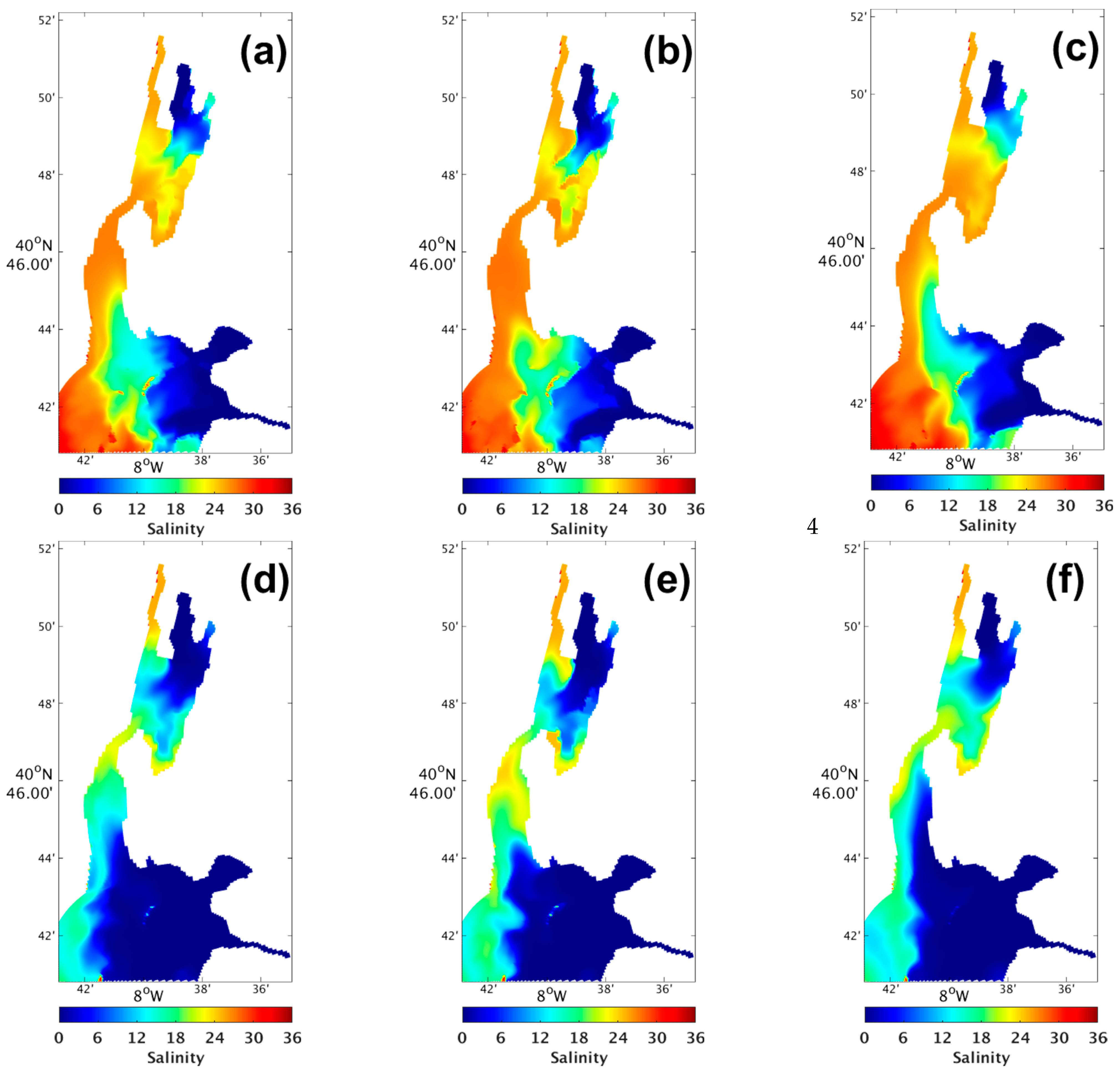
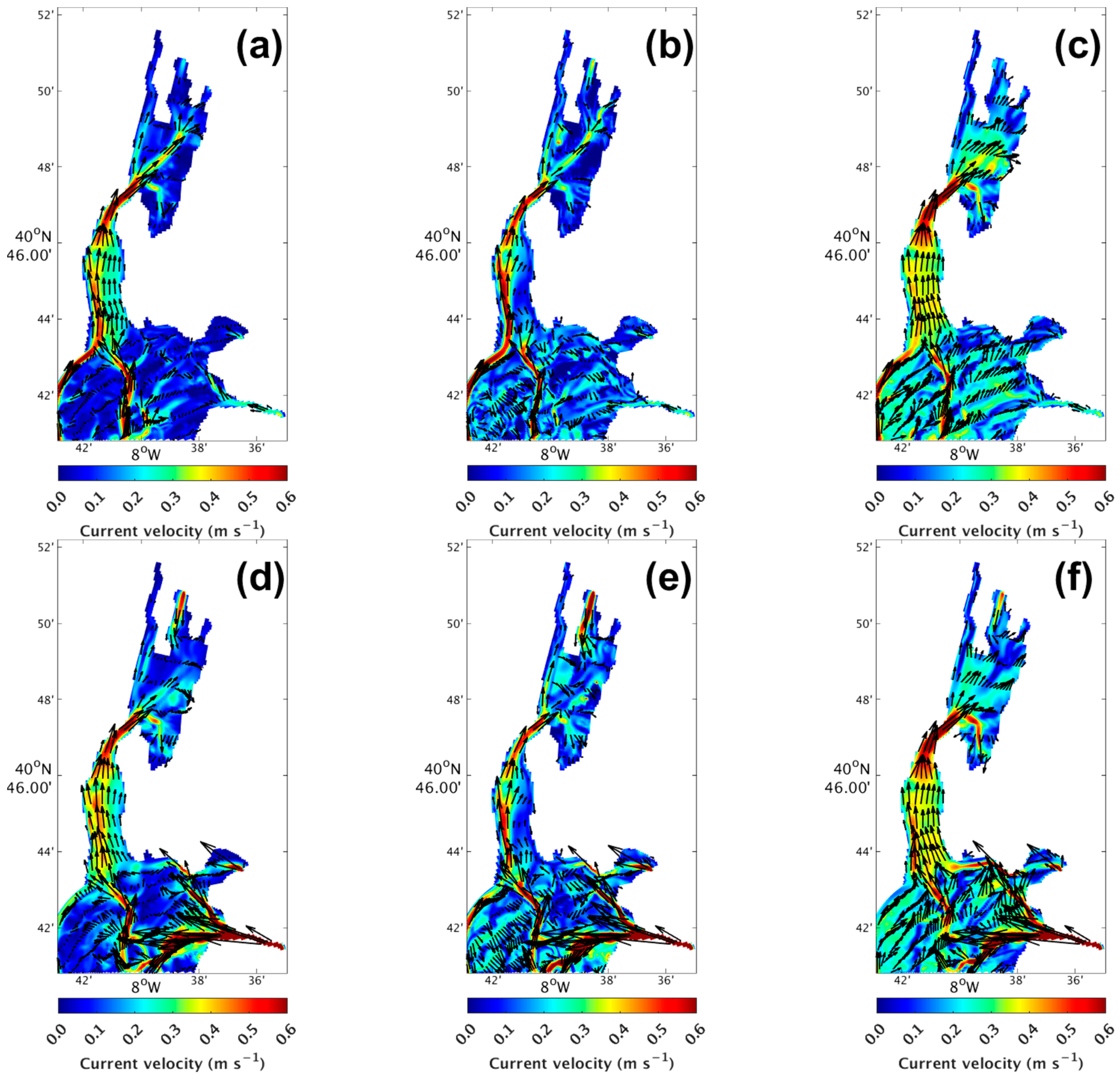
• The Espinheiro channel behaves as a partially mixed estuary, with salinity stratification found on the interface between the ocean water and freshwater masses, and increasing with the freshwater runoff. The local wind action mixture the water column and destroys salinity stratification, being the channel well-mixed for extreme wind scenarios, although it is not able to completely mix the water column under extreme freshwater runoff scenarios. NW storms push the estuarine front downstream, while SW storms are more effective than NW storms in destroying salinity stratification;
• Ílhavo channel behaves as a well-mixed estuary regardless of the freshwater runoff and wind conditions. The salinity intrusion is pushed downstream as the freshwater runoff increases, being the channel completely filled with freshwater under extreme scenarios;
• Mira channel generally behaves as a well-mixed estuary, but can present salinity stratification in the connection between the channel and the inlet for extreme freshwater scenarios. Windstorm scenarios are able to destroy the aforementioned stratification, and SW windstorms push the salinity intrusion downstream;
• São Jacinto channel presented perhaps the most interesting features, revealing an unusual estuarine pattern, with low salinity water masses midway of the channel and higher salinity water masses trapped upstream. It was found that this pattern is due to the advection of a freshwater plume generated by the Vouga and Antuã rivers. SW storms favour upstream currents that push the freshwater plume inward, while NW storms retain the plume outside the São Jacinto channel.

In summary, this work provides the first insights into the Ria de Aveiro lagoon’s horizontal and vertical salinity features under extreme freshwater runoff and wind events through a pioneering 3D implementation of a numerical model that comprised the entire Ria de Aveiro lagoon, covering the main lagoon’s channels which were not subject to intensive research on the hydrographic features before. It would be of great interest to increase the vertical sampling coverage of the lagoon’s main channels, namely Ílhavo, Mira, and São Jacinto, where vertical coverage is very poor, and therefore the results of this work should be taken carefully. This would allow for achieving a better validation of the model implementation developed. Due to the great importance of freshwater runoff in the establishment of salinity patterns, continuous monitoring of the lagoon’s five main tributaries should be considered and would also lead to more accurate results. It could also be of great interest that similar research was performed but with a focus on the impact of extreme weather events on water temperature vertical and horizontal patterns of the Ria de Aveiro lagoon and other estuaries and coastal lagoons worldwide.

References

- Kjerfve, B.; Magill, K.E. Geographic and Hydrodynamic Characteristics of Shallow Coastal Lagoons. Mar. Geol. 1989, 88, 187–199. [Google Scholar] [CrossRef]
- Kjerfve, B. Chapter 1 Coastal Lagoons. In Elsevier Oceanography Series; Kjerfve, B., Ed.; Coastal Lagoon Processes; Elsevier: Amsterdam, The Netherlands, 1994; Volume 60, pp. 1–8. [Google Scholar]
- Smith, N.P. Chapter 4 Water, Salt and Heat Balance of Coastal Lagoons. In Elsevier Oceanography Series; Kjerfve, B., Ed.; Coastal Lagoon Processes; Elsevier: Amsterdam, The Netherlands, 1994; Volume 60, pp. 69–101. [Google Scholar]
- Ji, X.; Sheng, J.; Tang, L.; Liu, D.; Yang, X. Process Study of Circulation in the Pearl River Estuary and Adjacent Coastal Waters in the Wet Season Using a Triply Nested Circulation Model. Ocean Model. 2011, 38, 138–160. [Google Scholar] [CrossRef]
- Xu, J.; Long, W.; Wiggert, J.D.; Lanerolle, L.W.J.; Brown, C.W.; Murtugudde, R.; Hood, R.R. Climate Forcing and Salinity Variability in Chesapeake Bay, USA. Estuaries Coasts 2012, 35, 237–261. [Google Scholar] [CrossRef]
- Okpeitcha, O.V.; Chaigneau, A.; Morel, Y.; Stieglitz, T.; Pomalegni, Y.; Sohou, Z.; Mama, D. Seasonal and Interannual Variability of Salinity in a Large West-African Lagoon (Nokoué Lagoon, Benin). Estuar. Coast. Shelf Sci. 2022, 264, 107689. [Google Scholar] [CrossRef]
- Moller, O.O.; Castaing, P.; Salomon, J.-C.; Lazure, P. The Influence of Local and Non-Local Forcing Effects on the Subtidal Circulation of Patos Lagoon. Estuaries 2001, 24, 297–311. [Google Scholar] [CrossRef]
- Castelao, R.M.; Moller, O.O., Jr. A Modeling Study of Patos Lagoon (Brazil): Flow Response to Idealized Wind and River Discharge: Dynamical Analysis. Braz. J. Oceanogr. 2006, 54, 1–17. [Google Scholar] [CrossRef]
- Andrade, M.M.; Abreu, P.C.; Ávila, R.A.; Möller, O.O. Importance of Winds, Freshwater Discharge and Retention Time in the Space–Time Variability of Phytoplankton Biomass in a Shallow Microtidal Estuary. Reg. Stud. Mar. Sci. 2022, 50, 102161. [Google Scholar] [CrossRef]
- Marin Jarrin, M.J.; Sutherland, D.A. Wind Effects on the Circulation of a Geometrically Complex Small Estuary. Estuar. Coast. Shelf Sci. 2022, 278, 108092. [Google Scholar] [CrossRef]
- Zemlys, P.; Ferrarin, C.; Umgiesser, G.; Gulbinskas, S.; Bellafiore, D. Investigation of Saline Water Intrusions into the Curonian Lagoon (Lithuania) and Two-Layer Flow in the Klaipeda Strait Using Finite Element Hydrodynamic Model. Ocean Sci. 2013, 9, 573–584. [Google Scholar] [CrossRef] [Green Version]
- Scully, M.E.; Friedrichs, C.; Brubaker, J. Control of Estuarine Stratification and Mixing by Wind-Induced Straining of the Estuarine Density Field. Estuaries 2005, 28, 321–326. [Google Scholar] [CrossRef]
- Silva, F.; Duck, R. Historical Changes of Bottom Topography and Tidal Amplitude in the Ria de Aveiro, Portugal—Trends for Future Evolution. Clim. Res 2001, 18, 17–24. [Google Scholar] [CrossRef] [Green Version]
- De Jonge, V.N.; Schuttelaars, H.M.; van Beusekom, J.E.E.; Talke, S.A.; de Swart, H.E. The Influence of Channel Deepening on Estuarine Turbidity Levels and Dynamics, as Exemplified by the Ems Estuary. Estuar. Coast. Shelf Sci. 2014, 139, 46–59. [Google Scholar] [CrossRef]
- Ralston, D.K.; Talke, S.; Geyer, W.R.; Al-Zubaidi, H.A.M.; Sommerfield, C.K. Bigger Tides, Less Flooding: Effects of Dredging on Barotropic Dynamics in a Highly Modified Estuary. J. Geophys. Res. Oceans 2019, 124, 196–211. [Google Scholar] [CrossRef] [Green Version]
- Dias, J.M.; Pereira, F.; Picado, A.; Lopes, C.L.; Pinheiro, J.P.; Lopes, S.M.; Pinho, P.G. A Comprehensive Estuarine Hydrodynamics-Salinity Study: Impact of Morphologic Changes on Ria de Aveiro (Atlantic Coast of Portugal). J. Mar. Sci. Eng. 2021, 9, 234. [Google Scholar] [CrossRef]
- Salles, P.; Valle-Levinson, A.; Sottolichio, A.; Senechal, N. Wind-Driven Modifications to the Residual Circulation in an Ebb-Tidal Delta: Arcachon Lagoon, Southwestern France. J. Geophys. Res. Oceans 2015, 120, 728–740. [Google Scholar] [CrossRef]
- Vaz, N.; Dias, J. Residual Currents and Transport Pathways in the Tagus Estuary, Portugal: The Role of Freshwater Discharge and Wind. J. Coast. Res. 2014, 70, 610–615. [Google Scholar] [CrossRef]
- Malta, E.; Stigter, T.; Pacheco, A.; Dill, A.M.M.; Tavares, D.; Santos, R. Effects of External Nutrient Sources and Extreme Weather Events on the Nutrient Budget of a Southern European Coastal Lagoon. Estuaries Coasts 2016, 40, 419–436. [Google Scholar] [CrossRef] [Green Version]
- Ribeiro, A.F.; Sousa, M.; Picado, A.; Ribeiro, A.S.; Dias, J.M.; Vaz, N. Circulation and Transport Processes during an Extreme Freshwater Discharge Event at the Tagus Estuary. J. Mar. Sci. Eng. 2022, 10, 1410. [Google Scholar] [CrossRef]
- Alekseenko, E.; Roux, B. Numerical Simulation of the Wind Influence on Bottom Shear Stress and Salinity Fields in Areas of Zostera Noltei Replanting in a Mediterranean Coastal Lagoon. Prog. Oceanogr. 2018, 163, 147–160. [Google Scholar] [CrossRef] [Green Version]
- Fernandes, E.H.L.; Dyer, K.R.; Moller, O.O.; Niencheski, L.F.H. The Patos Lagoon Hydrodynamics during an El Niño Event (1998). Cont. Shelf Res. 2002, 22, 1699–1713. [Google Scholar] [CrossRef]
- Dias, J.M. Contribution to the Study of the Ria de Aveiro Hydrodynamics. Ph.D. Thesis, Universidade de Aveiro, Aveiro, Portugal, 2001. [Google Scholar]
- Vaz, N. Study of Heat and Salt Transport Processes in the Espinheiro Channel (Ria de Aveiro). Ph.D. Thesis, Universidade de Aveiro, Aveiro, Portugal, 2007. [Google Scholar]
- Vargas, C.I.C.; Vaz, N.; Dias, J.M. An Evaluation of Climate Change Effects in Estuarine Salinity Patterns: Application to Ria de Aveiro Shallow Water System. Estuar. Coast. Shelf Sci. 2017, 189, 33–45. [Google Scholar] [CrossRef]
- Lopes, J.F.; Dias, J.M. Residual Circulation and Sediment Distribution in the Ria de Aveiro Lagoon, Portugal. J. Mar. Syst. 2007, 68, 507–528. [Google Scholar] [CrossRef]
- Ulbrich, U.; Christoph, M.; Pinto, J.G.; Corte-Real, J. Dependence of Winter Precipitation over Portugal on NAO and Baroclinic Wave Activity. Int. J. Climatol. 1999, 19, 379–390. [Google Scholar] [CrossRef]
- Raible, C.C. On the Relation between Extremes of Midlatitude Cyclones and the Atmospheric Circulation Using ERA40. Geophys. Res. Lett. 2007, 34, L07703. [Google Scholar] [CrossRef]
- Betts, N.L.; Orford, J.D.; White, D.; Graham, C.J. Storminess and Surges in the Southwestern Approaches of the Eastern North Atlantic: The Synoptic Climatology of Recent Extreme Coastal Storms. Mar. Geol. 2004, 210, 227–246. [Google Scholar] [CrossRef]
- Liberato, M.L.R.; Pinto, J.G.; Trigo, R.M.; Ludwig, P.; Ordóñez, P.; Yuen, D.; Trigo, I.F. Explosive Development of Winter Storm Xynthia over the Subtropical North Atlantic Ocean. Nat. Hazards 2013, 13, 2239–2251. [Google Scholar] [CrossRef] [Green Version]
- Liberato, M.L.R. The 19 January 2013 Windstorm over the North Atlantic: Large-Scale Dynamics and Impacts on Iberia. Weather Clim. Extrem. 2014, 5, 16–28. [Google Scholar] [CrossRef] [Green Version]
- Ferreira, J.A.; Pradhan, P.K.; Liberato, M.L.R. Impacts of extratropical cyclone Stephanie assessed by a high resolution model setting. In Proceedings of the International Conference Mathematics and Engineering in Marine and Earth Problems (MEME’2014), Aveiro, Portugal, 22–25 July 2014; Aveiro University: Aveiro, Portugal, 2014; pp. 92–97. [Google Scholar]
- Pinheiro, J.P.; Lopes, C.L.; Ribeiro, A.S.; Sousa, M.C.; Dias, J.M. Tide-Surge Interaction in Ria de Aveiro Lagoon and Its Influence in Local Inundation Patterns. Cont. Shelf Res. 2020, 200, 104132. [Google Scholar] [CrossRef]
- Silveira, F.; Lopes, C.L.; Pinheiro, J.P.; Pereira, H.; Dias, J.M. Coastal Floods Induced by Mean Sea Level Rise—Ecological and Socioeconomic Impacts on a Mesotidal Lagoon. J. Mar. Sci. Eng. 2021, 9, 1430. [Google Scholar] [CrossRef]
- Lopes, C.; Azevedo, A.; Dias, J. Flooding Assessment under Sea Level Rise Scenarios: Ria de Aveiro Case Study. J. Coast. Res. 2013, 65, 766–771. [Google Scholar] [CrossRef]
- Dias, J.M.; Lopes, J.; Dekeyser, I. Hydrological Characterisation of Ria de Aveiro, Portugal, in Early Summer. Oceanol. Acta 1999, 22, 473–485. [Google Scholar] [CrossRef] [Green Version]
- Lopes, C.L. Flood Risk Assessment in Ria de Aveiro Under Present and Future Scenarios. Ph.D. Thesis, Universidade de Aveiro, Aveiro, Portugal, 2016. [Google Scholar]
- Lopes, C.; Plecha, S.; Silva, P.; Dias, J. Influence of Morphological Changes in a Lagoon Flooding Extension: Case Study of Ria de Aveiro (Portugal). J. Coast. Res. 2013, 165, 1158–1163. [Google Scholar] [CrossRef]
- Araújo, I.B.; Dias, J.; Pugh, D.T. Model Simulations of Tidal Changes in a Coastal Lagoon, the Ria de Aveiro (Portugal). Cont. Shelf Res. 2008, 28, 1010–1025. [Google Scholar] [CrossRef]
- Silva, J.F. Circulação Da Água Na Ria de Aveiro: Contribuição Para o Estudo Da Qualidade Da Água. Ph.D. Thesis, Universidade de Aveiro, Aveiro, Portugal, 1994. [Google Scholar]
- Moreira, M.H.; Queiroga, H.; Machado, M.M.; Cunha, M.R. Environmental Gradients in a Southern Europe Estuarine System: Ria de Aveiro, Portugal Implications for Soft Bottom Macrofauna Colonization. Netherland J. Aquat. Ecol. 1993, 27, 465–482. [Google Scholar] [CrossRef]
- Dias, J.M.; Lopes, J.F.; Dekeyser, I. Tidal Propagation in Ria de Aveiro Lagoon, Portugal. Phys. Chem. Earth Part B Hydrol. Ocean. Atmos. 2000, 25, 369–374. [Google Scholar] [CrossRef]
- Génio, L.; Sousa, A.; Vaz, N.; Dias, J.M.; Barroso, C. Effect of Low Salinity on the Survival of Recently Hatched Veliger of Nassarius Reticulatus (L.) in Estuarine Habitats: A Case Study of Ria de Aveiro. J. Sea Res. 2008, 59, 133–143. [Google Scholar] [CrossRef]
- Vicente, C.M. Caracterização Hidráulica e Aluvionar da Ria de Aveiro—Utilização de Modelos Hidráulicos no Estudo de Problemas. Jorn. Ria Aveiro 1985, 3, 41–58. [Google Scholar]
- Dias, J.M.; Fonseca, A.; Picado, A.; Lopes, C.L.; Silva, J.; Vaz, L.; Mendes, R.; Plecha, S. Estudos da Evolução e da Dinâmica Costeira e Estuarina da Ria de Aveiro no âmbito do Polis Litoral da Ria de Aveiro; 3rd Technical Report; Universidade de Aveiro: Aveiro, Portugal, 2011; 42p. [Google Scholar]
- Deltares. Delft3D-FLOW User Manual; Deltares: Delft, The Netherlands, 2022. [Google Scholar]
- Cavalinhos, R.; Correia, R.; Rosa, P.; Lillebo, A.I.; Pinheiro, L.M. Processed Multibeam Bathymetry Data Collected around the Ria de Aveiro, Portugal, Onboard the NEREIDE Research Vessel [Data Set]; Zenodo: Aveiro, Portugal, 2020. [Google Scholar]
- EMODnet Bathymetry Consortium. EMODnet Digital Bathymetry (DTM 2020). Available online: https://sextant.ifremer.fr/record/bb6a87dd-e579-4036-abe1-e649cea9881a/ (accessed on 2 January 2023).
- Matsumoto, K.; Takanezawa, T.; Ooe, M. Ocean Tide Models Developed by Assimilating TOPEX/POSEIDON Altimeter Data into Hydrodynamical Model: A Global Model and a Regional Model around Japan. J. Oceanogr. 2000, 56, 567–581. [Google Scholar] [CrossRef]
- Copernicus Marine Service. Atlantic-Iberian Biscay Irish- Ocean Physics Reanalysis. Available online: https://data.marine.copernicus.eu/product/IBI_MULTIYEAR_BGC_005_003/description (accessed on 11 January 2023). [CrossRef]
- Hersbach, H.; Bell, B.; Berrisford, P.; Hirahara, S.; Horányi, A.; Muñoz-Sabater, J.; Nicolas, J.; Peubey, C.; Radu, R.; Schepers, D.; et al. The ERA5 Global Reanalysis. Q. J. R. Meteorol. Soc. 2020, 146, 1999–2049. [Google Scholar] [CrossRef]
- Krysanova, V.; Meiner, A.; Roosaare, J.; Vasilyev, A. Simulation Modelling of the Coastal Waters Pollution from Agricultural Watershed. Ecol. Model. 1989, 49, 7–29. [Google Scholar] [CrossRef]
- Stefanova, A.; Krysanova, V.; Hesse, C.; Lillebø, A.I. Climate Change Impact Assessment on Water Inflow to a Coastal Lagoon: The Ria de Aveiro Watershed, Portugal. Hydrol. Sci. J. 2015, 60, 929–948. [Google Scholar] [CrossRef]
- Dias, J.; Picado, A. Impact of Morphologic Anthropogenic and Natural Changes in Estuarine Tidal Dynamics. J. Coast. Res. 2011, 64, 1490–1494. [Google Scholar]
- Stow, C.A.; Jolliff, J.; McGillicuddy, D.J.; Doney, S.C.; Allen, J.I.; Friedrichs, M.A.M.; Rose, K.A.; Wallhead, P. Skill Assessment for Coupled Biological/Physical Models of Marine Systems. J. Mar. Syst. 2009, 76, 4–15. [Google Scholar] [CrossRef] [Green Version]
- Warner, J.C.; Geyer, W.R.; Lerczak, J.A. Numerical Modeling of an Estuary: A Comprehensive Skill Assessment. J. Geophys. Res. Ocean. 2005, 110, C05001. [Google Scholar] [CrossRef]
- Arnold, J.G.; Allen, P.M.; Bernhardt, G. A Comprehensive Surface-Groundwater Flow Model. J. Hydrol. 1993, 142, 47–69. [Google Scholar] [CrossRef]
- Vaz, N.; Dias, J.; Martins, I. Dynamics of a Temperate Fluvial Estuary in Early Winter. Glob. Int. J. 2005, 7, 18. [Google Scholar]
- Vaz, N.; Dias, J.M. Hydrographic Characterization of an Estuarine Tidal Channel. J. Mar. Syst. 2008, 70, 168–181. [Google Scholar] [CrossRef]
- Ferreira, J.A.; Liberato, M.L.R.; Ramos, A.M. On the Relationship between Atmospheric Water Vapour Transport and Extra-Tropical Cyclones Development. Phys. Chem. Earth. 2016, 94, 56–65. [Google Scholar] [CrossRef]
- Jassby, A.D.; Kimmerer, W.J.; Monismith, S.G.; Armor, C.; Cloern, J.E.; Powell, T.M.; Schubel, J.R.; Vendlinski, T.J. Isohaline Position as a Habitat Indicator for Estuarine Populations. Ecol. Appl. 1995, 5, 272–289. [Google Scholar] [CrossRef] [Green Version]
- Díez-Minguito, M.; Contreras, E.; Polo, M.J.; Losada, M.A. Spatio-Temporal Distribution, along-Channel Transport, and Post-Riverflood Recovery of Salinity in the Guadalquivir Estuary (SW Spain). J. Geophys. Res. Ocean. 2013, 118, 2267–2278. [Google Scholar] [CrossRef]
- Andrews, S.W.; Gross, E.S.; Hutton, P.H. Modeling Salt Intrusion in the San Francisco Estuary Prior to Anthropogenic Influence. Cont. Shelf Res. 2017, 146, 58–81. [Google Scholar] [CrossRef]
- Guerra-Chanis, G.E.; Reyes-Merlo, M.; Díez-Minguito, M.; Valle-Levinson, A. Saltwater Intrusion in a Subtropical Estuary. Estuar. Coast. Shelf Sci. 2019, 217, 28–36. [Google Scholar] [CrossRef]
- Dias, J.M.; Sousa, M.C.; Bertin, X.; Fortunato, A.B.; Oliveira, A. Numerical Modeling of the Impact of the Ancão Inlet Relocation (Ria Formosa, Portugal). Environ. Model. Softw. 2009, 24, 711–725. [Google Scholar] [CrossRef]
- Mendes, R.; Vaz, N.; Dias, J. Numerical Modeling Changes Induced by the Low Lying Areas Adjacent to Ria de Aveiro. J. Coast. Res. 2011, 64, 1125–1129. [Google Scholar]
- Vaz, N.; Dias, J.M.; Leitão, P.; Martins, I. Horizontal Patterns of Water Temperature and Salinity in an Estuarine Tidal Channel: Ria de Aveiro. Ocean Dyn. 2005, 55, 416–429. [Google Scholar] [CrossRef] [Green Version]
- Vaz, N.; Miguel Dias, J.; Chambel Leitão, P. Three-Dimensional Modelling of a Tidal Channel: The Espinheiro Channel (Portugal). Cont. Shelf Res. 2009, 29, 29–41. [Google Scholar] [CrossRef]