A COLREGs-Compliant Ship Collision Avoidance Decision-Making Support Scheme Based on Improved APF and NMPC

Abstract

In this paper, combined with the improved artificial potential field (IAPF) method and the nonlinear model predictive control (NMPC) algorithm, a collision avoidance decision-making support scheme considering ship maneuverability and the International Regulations for Preventing Collisions at Sea (COLREGs) is proposed. First, to comply with the requirements of COLREGs, an improved repulsive potential field is presented for different encounter scenarios when the ship detects the risk of collision, and the coordinated ship domain is applied to provide safety criteria for collision avoidance. Then, by transforming the MMG model to a discrete-time nonlinear system, the NMPC is utilized to predict the future state of the ship according to the current state, and the IAPF method is incorporated to calculate the potential field in each future state as the objective function. Following this approach, the action taken to avoid collision is more effective, the ship motion in avoiding collision is more accurate, and the collision avoidance decision making is more reasonable. Finally, two simulation examples of multi-ship encounter scenarios are applied to illustrate the merits and effectiveness of the proposed collision avoidance decision-making support scheme.

1. Introduction

In the past decades, due to the high incidence and serious consequences of ship collision, preventing collision accidents has always been in the spotlight among practitioners and researchers. Through the analysis and investigation of a large number of accident reports, researchers have come to a common conclusion that human factors are the main cause of ship collision accidents [1]. To mitigate or even eliminate the impact of human factors, the research on ship anti-collision mainly focuses on assisting human and autonomous collision avoidance [2].

Ship path planning methods are always presented to realize autonomous collision avoidance and navigation. The application of A-star [3], rapid-exploring random tree [4] and other algorithms [5] in ship path planning has been developed for many years. Comparatively, these studies take into account static obstacles and ignore dynamic obstacles. The artificial potential field (APF) method, which was first formally applied [6] to real-time collision avoidance of robots in known static environments, has gradually attracted the attention of scholars and is widely used in path planning, such as unmanned aerial vehicle (UAV) [7], autonomous vehicle [8], etc. Due to its ability to deal with static and dynamic obstacles, the APF method is also applied in ship collision avoidance [9,10]. In the process of collision avoidance, the requirements of some key rules in COLREGs are usually taken into account. A COLREGs-constrained multi-ship real-time autonomous collision avoidance decision-making algorithm based on improved APF was proved to have the advantages of fast calculation speed and strong robustness [11]. The repulsive potential field was modified depending on the relevant descriptions of COLREGs for different encounter scenarios, and a guidance strategy was proposed for an underactuated unmanned surface vehicle (USV) based on improved APF [12]. However, the traditional APF method is prone to falling into local optima in path planning. Some researchers gradually focus on combining APF and other algorithms to overcome the drawbacks of traditional APF. A collision avoidance scheme based on APF and deep Q-learning network (DQN) was presented, incorporating the resultant force of APF and the requirements of COLREGs into the reward function of DQN [13]. To improve the feasibility and reasonability of an anti-collision scheme, a path planning algorithm considering the requirements of COLREGs and combining modified velocity obstacle (VO) and APF was proposed [14]. However, compared with the traditional APF, the repulsive potential field for three encounter scenarios should be developed and improved according to the rules of COLREGs.

At present, a lot of research works on path planning methods ignore whether the obtained path is prone to being tracked by the ship. In other words, path planning should also fully consider the ship motion control algorithm and tracking effect. Due to its outstanding performance in predicting the future state and dealing with multi-constraint problems, model predictive control (MPC) was widely utilized in ship motion control [15,16]. MPC is a control method based on the object, and its control accuracy is directly related to the model’s accuracy. For a nonlinear system, linearizing the nonlinear system and then utilizing MPC control can simplify the control process and improve the calculation speed, but it may also lead to low control accuracy, poor controller robustness and other consequences [17]. For ship trajectory tracking and obstacle avoidance in uncertain external environmental disturbance, a trajectory tracking control method based on nonlinear model predictive control (NMPC) was proposed to ensure the high control accuracy and strong robustness of the controller [18]. A trajectory tracking with obstacle avoidance algorithm, incorporating an event-triggered mechanism into the NMPC design, was presented, which can ensure good obstacle avoidance effect and reduce the computational burden [19]. Obviously, to improve control accuracy and controller robustness, the NMPC scheme is more suitable for ship motion control than the MPC scheme.

Based on the excellent tracking performance of the MPC scheme, the combination of MPC and APF has gradually attracted scholars’ attention in collision avoidance. A repulsive potential field was included in an NMPC method to avoid collision with obstacles and control multiple USV in arbitrary formations [20]. However, this scheme ignores the COLREGs and only considers static obstacle avoidance. Considering the constraints of ship maneuverability and the requirements of COLREGs, a novel motion planning method based on MPC and APF was proposed for multi-object collision avoidance [21], which can solve the problem of easily falling into local optima in traditional APF. It is worth noting that the ship kinematic model used was obtained by ignoring the influence of sway velocity components and simplifying the hydrodynamic parameters and derivatives of the model [22]. This model is mainly applied to describe the ship maneuvering characteristics of a small rudder angle, while the accuracy of describing the ship maneuvering characteristics of a large rudder angle is insufficient [23].

In particular, the maneuvering modeling group (MMG) model is one of the famous and high-precision mathematical models for ship maneuvering presented by the Japanese Towing Tank Conference (JTTC) [24]. To describe the ship maneuvering motion characteristics for a ship meeting at a close range, a collision avoidance dynamic support model was proposed [25] by combining a three-degrees-of-freedom (DOF) MMG model, a control algorithm and a collision avoidance parameter mathematical model, which demonstrates the importance and necessity of considering ship maneuvering motion characteristics in collision avoidance. In addition, ship maneuvering motion characteristics should be considered when providing the safety criteria for collision avoidance. The coordinated ship domain, which was proposed by taking into account ship maneuverability and mutual interaction of meeting ships [26], can provide more reasonable safety criteria than other ship domains.

Motivated by the above observation, this paper proposes a collision avoidance decision-making support scheme by combining the IAPF method and the NMPC algorithm, which considers the COLREGs and ship maneuverability. The main contributions are summarized as follows.

(1)

According to some critical rules of COLREGs, the repulsive potential field for three encounter scenarios, i.e., head-on, crossing and overtaking situations, is developed and improved in this paper.

(2)

A standard 3 DOF MMG model is applied to denote ship maneuvering motion characteristics in the process of collision avoidance, and then, a collision avoidance decision-making support scheme is proposed by incorporating the IAPF method into the NMPC design.

(3)

The coordinated ship domain, which considers ship maneuverability and mutual interaction of meeting ships, is applied to determine the safety criteria in the process of collision avoidance.

The rest of the article is organized as follows. Section 2 describes the IAPF method considering the requirements of COLREGs and introduces the coordinated ship domain. Section 3 introduces the MMG model and gives the NMPC design procedure. Section 4 shows the effectiveness of the presented collision avoidance decision-making support scheme. Section 5 presents the conclusions.

2. Improved Artificial Potential Field Method

As a path planning method with simple principles and practical solid application, the APF is widely used in collision avoidance. The core idea of the APF method is to regard the motion of a ship in an actual environment as the motion in a virtual potential energy field, where the ship is affected by all kinds of forces. The attractive force of the goal point drives it toward the goal point. On the contrary, the obstacles in the environment produce a repulsive force to prevent the ship from colliding with obstacles. Therefore, the resultant force will bring the ship closer to the target point and away from the obstacles. In addition, when the APF is combined with MPC, instead of calculating the attractive and repulsive forces, the total potential field is calculated [21], and the path with the gradient of steepest descent in the total potential field is the optimal path.

2.1. Attractive Potential Field

The attractive potential U_att(p) is defined as a function of the relative distance between the own ship (OS) and the goal point.

$$U_{att}(p)=\frac{1}{2}{k}_{att}\rho {(p_{os},p_g)}^2$$

(1)

where k_att is the attractive potential field coefficient; p_os, p_g are the position of the OS and the goal point, respectively. ρ(p_os, p_g) is the distance between the own ship and the goal point.

2.2. COLREGs-Compliant Repulsive Potential Field

Collision risk assessment is a vitally important part of the process of collision avoidance. The closest point of approach (CPA) method is selected to assess collision risk and decide whether to take avoiding action [27]. Meanwhile, in the process of actual ship collision avoidance, the requirements of COLREGs cannot be ignored. Based on the above-mentioned statement [12], this paper proposes an improved repulsive potential field, which considers risk and complies with COLREGs. There are different ways to improve the different encounter situations. Primarily, according to Rule 14 of COLREGs [28], which describes the action of two power-driven vessels in a head-on situation, it can be found that the own ship shall alter course to the starboard and pass on the port side of the target ship (TS). Therefore, the repulsive potential field is constructed according to the change in the distance between the OS and the TS, and the distance from the OS to the longitudinal centerline of the TS. Then, some settings are added, so that the own ship’s actions can avoid collision and comply with the requirements of COLREGs. The repulsive potential field generated by the TS is as follows:

$$\left\{\begin{array}{l}{U}_{rep}=\frac{1}{2}{k}_{rep}\frac{{(d_s(p,p_L)+d_1)}^2}{\rho {(p_{os},p_t)}^2}\\ if\rho (p_{os},p_t)\le l_t,d_s(p,p_L)>-d_1 and \mathrm{TCPA}\ge 0\\ \\ 0\mathrm{others}\end{array}\right.$$

(2)

where k_rep is the repulsive potential field coefficient; ρ(p_os, p_t) is the distance between the OS and the TS; l_t is the influence radius of the TS; d₁ is a preset reference distance in a head-on situation; d_s(p, p_L) denotes the distance from the OS to the longitudinal centerline of the TS. If the OS is on the port side of the TS, d_s(p, p_L) is a negative value; otherwise, it is a positive value.

Similarly, according to Rule 15 of COLREGs, which describes the action of two power-driven vessels in a crossing situation, it can be found that the give-way ship shall avoid crossing ahead of the other vessel. Assuming the OS is a give-way ship, the repulsive potential field is constructed according to the change in the distance from the OS to the TS and the distance from the OS to the transverse centerline of the TS. The repulsive potential field of the TS when the OS needs to avoid the TS in a crossing situation is as follows:

$$\left\{\begin{array}{l}{U}_{rep}=\frac{1}{2}{k}_{rep}\frac{{(d_s(p,p_T)+d_2)}^2}{\rho {(p_{os},p_t)}^2}\\ if\rho (p_{os},p_t)\le l_0,d_s(p,p_T)>-d_2 and \mathrm{TCPA}\ge 0\\ \\ 0\mathrm{others}\end{array}\right.$$

(3)

where d₂ is a preset reference distance in a crossing situation; d_s(p, p_T) denotes the distance from the OS to the transverse centerline of the TS. If the OS is on the stern side of the TS, d_s(p, p_T) is a negative value; otherwise, it is a positive value.

For an overtaking situation, according to Rule 13 of COLREGs, it can be found that the give-way ship can alter the course to the starboard or the port depending on the navigation conditions. When the OS is a give-way ship, the repulsive potential field of the TS is constructed according to the change in the distance between the OS and the TS, and the distance from the OS to the transverse centerline of the TS as follows:

$$\left\{\begin{array}{l}{U}_{rep}=\frac{1}{2}{k}_{rep}\frac{{(d_3-d_v(p,p_L))}^2}{\rho {(p_{os},p_t)}^2}\\ if\rho (p_{os},p_t)\le l_0,d_v(p,p_L)<d_3 and \mathrm{TCPA}\ge 0\\ \\ 0\mathrm{others}\end{array}\right.$$

(4)

where d₃ is a preset reference distance in an overtaking situation; d_v(p, p_L) denotes the vertical distance between the OS and the longitudinal centerline of the TS, which is a positive value.

This paper aims to find a path with the gradient of steepest descent in the total potential field. Here, the total potential field at the ith moment is used for analysis, and the ship is assumed to be within the influence range of the N_t target ships. The total potential field P_f,i at the ith moment is expressed as follows:

$$P_{f,i}=P_{g,i}+{\displaystyle \sum _{n=1}^{N_t}{P}_{t,i,n}}$$

(5)

where P_g,i is the potential field of the goal at the ith moment; P_t,i,n is the potential field of the target ship n at the ith moment.

2.3. Coordinated Ship Domain

Over the past decades, the research on the ship domain of marine traffic engineering has received much attention because the ship domain plays a vital role in the navigational safety of ships. The concept of the ship domain was first proposed as an “effective domain” [29], which means the domain around a ship under way, which most navigators of the following ships would avoid invading. Then, the ship domain was further regarded as the effective area around a ship, which a navigator would like to keep free for other ships and stationary obstacles [30]. Through years of progress, a large number of ship domains have been presented for various purposes, which were classified into three classes in a geometrical manner, i.e., circle, ellipse and polygon.

The shape and size of the ship domain model depend mainly on the characteristics of the ship, such as length and speed. However, the difference in the size of the ship domain between the two vessels can lead to a different identification of the danger level. Therefore, the coordinated ship domain is applied [26], which considers the cooperation between ships and the influence of the ship’s advance on the setting of a safe distance. In addition, the distance from the middle of the ship to the bow of the ship is also a major factor and should be considered when ships meet at close quarters. Hence, the radius of the ship domain R_c is expressed as

$$R_c=D_{center}+T{A}_{\max }$$

(6)

where D_center denotes the distance between the center of the ship domain and the bow of the ship, which is equal to 0.5L_max; TA_max denotes the maximum ship length of the universal advance and the tactical diameter based on turning circle maneuver data, which is equal to 4.0L_max. Therefore, the size of the ship domain can be expressed as

$$R_c=0.5L_{\max }+4L_{\max }=4.5L_{\max }$$

(7)

where L_max is the maximum length of the ships, which are involved in an encounter situation, which is expressed as follows

$$L_{\max }=\max (L_1,L_2,\dots ,L_n),(n=1,2,\dots ,N)$$

(8)

When multiple ships are meeting on the open sea, the coordinated ship domain is applied to the own ship and the target ships simultaneously to ensure passage at a safe distance, i.e., multiple meeting ships use the same ship domain.

3. Collision Avoidance Decision-Making Support Scheme Based on IAPF and NMPC

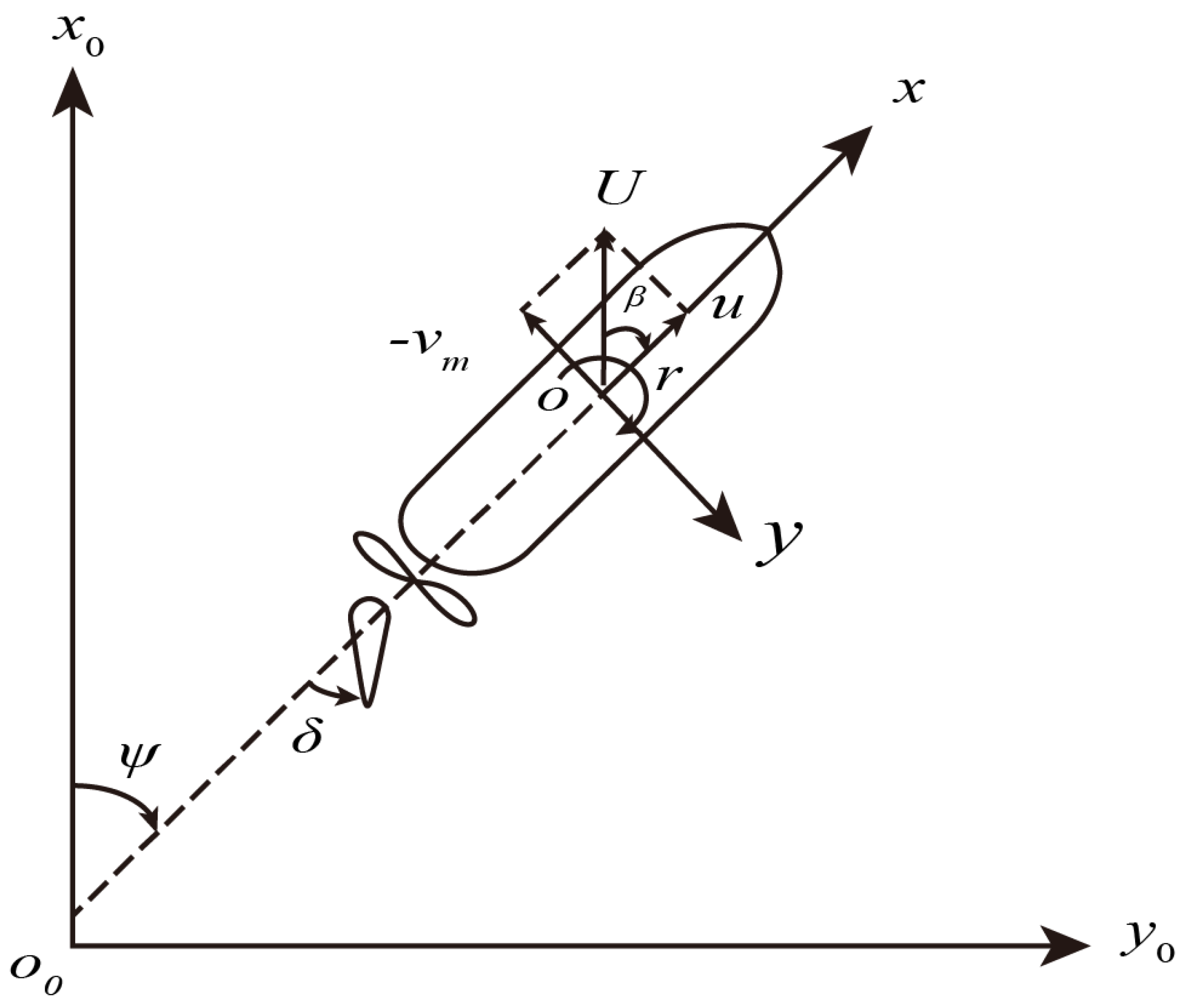
3.1. Maneuvering Modeling Group (MMG) Model

Figure 1 shows the body-fixed coordinate system o-xyz within the space-fixed coordinate system o₀-x₀y₀z₀, and the origin o is located in the mid-ship of the ship.

The variations in the ship heading angle ψ and ship position (x, y) in the space-fixed coordinate system are expressed as

$$\left\{\begin{array}{l}\dot{x}=u\cos \psi -v\sin \psi \\ \dot{y}=u\sin \psi +v\cos \psi \\ \dot{\psi }=r\end{array}\right.$$

(9)

$$v=v_m+x_{G}r$$

(10)

where u, v and r denote the surge velocity, sway velocity at the gravity and yaw rate, respectively; v_m and x_G are the sway velocity at mid-ship and the distance from the center of gravity to the mid-ship.

Concretely, the standard 3 DOF MMG motion equations are defined as follows:

$$\left\{\begin{array}{l}(m+m_x)\dot{u}-(m+m_y)v_{m}r-x_{G}m{r}^2=X_H+X_R+X_P\\ (m+m_y){\dot{v}}_m+(m+m_x)ur+x_{G}m\dot{r}=Y_H+Y_R\\ (I_{zG}+x_G^{2}m+J_z)\dot{r}+x_{G}m({\dot{v}}_m+ur)=N_H+N_R\end{array}\right.$$

(11)

where m, m_x, m_y, J_z and I_zG are the ship’s mass, the ship’s added mass in the o–x axis direction, the added mass in the o–y axis direction, the added moment of inertia around the mid-ship and the moment of inertia of the ship around the center of gravity, respectively. X, Y and N are the surge force, lateral force and yaw moment around the mid-ship; the subscripts H, R and P denote the ship hull, rudder and propeller, respectively. The force and the moment acting on the hull X_H, Y_H and N_H are defined as follows:

$$\left\{\begin{array}{l}{X}_H=(1/2)\rho L_{pp}d{U}^2{X}_H^{\prime }(v_m^{\prime },r^{\prime })\\ Y_H=(1/2)\rho L_{pp}d{U}^2{Y}_H^{\prime }(v_m^{\prime },r^{\prime })\\ N_H=(1/2)\rho L_{pp}^{2}d{U}^2{N}_H^{\prime }(v_m^{\prime },r^{\prime })\\ U=\sqrt{u^2+v_m^2}\end{array}\right.$$

(12)

where ρ, d, L_pp and U denote the water density, ship draft, ship length between the perpendiculars and the resultant velocity, respectively. $v_m^{\prime }$ is nondimensionalized by v_m/U, and r’ is nondimensionalized by rL_pp/U. The force acting on the propeller X_P is defined as

$$\left\{\begin{array}{l}{X}_p=(1-t_P)\rho n_p^2{D}_p^4(k_{t2}{J}_p^2+k_{t1}{J}_p+k_{t0})\\ J_P=u\left[1-w_{p0}\exp (C_0{(\beta -x_p^{\prime }{r}^{\prime })}^2)\right]/n_p{D}_p\\ \beta =\arctan (-v_m/u)\end{array}\right.$$

(13)

where δ, t_p, n_p, D_p and J_p denote the rudder angle, thrust deduction factor, propeller revolution, propeller diameter and propeller advanced ratio, respectively. k_t0, k_t1, k_t2 are the propeller thrust open water characteristic coefficients; w_p0, C₀, β and x_p denote the wake coefficient of the propeller in a straight moving direction, the experimental constant, the drift angle and the longitudinal coordinate of the propeller position, respectively. The force and the moment acting on the rudder X_R, Y_R and N_R are defined as follows:

$$\left\{\begin{array}{l}{X}_R=-0.5(1-t_R)\rho A_R(u_R^2+v_R^2)f_{\alpha }\sin {\alpha }_R\sin \delta \\ Y_R=-0.5(1-a_H)\rho A_R(u_R^2+v_R^2)f_{\alpha }\sin {\alpha }_R\cos \delta \\ N_R=-0.5(x_R+a_H{x}_H)\rho A_R(u_R^2+v_R^2)f_{\alpha }\sin {\alpha }_R\cos \delta \\ {\alpha }_R=\delta -{\tan }^{-1}(v_R/u_R)\approx \delta -v_R/u_R\end{array}\right.$$

(14)

where t_R, a_H, x_H and x_R denote the steering resistance deduction factor, the increase factor of the rudder force, the distance from the additional lateral force component to the mid-ship and the distance from the rudder to the mid-ship, respectively. A_R, α_R, f_α, u_R and v_R represent the profile area, the effective inflow angle, the lift gradient coefficient, the longitudinal and lateral inflow velocity of the rudder, respectively.

Meanwhile, consider the actual performance of the rudder as follows

$$\dot{\delta }=-(1/T_E)\delta +(1/T_E){\delta }_E$$

(15)

where T_E is the steering factor; δ_E denotes the order angle of the steering gear and also represents the actual input of the system.

3.2. Nonlinear Model Predictive Control Design

It can be seen from Equation (11) that the maneuvering equations are a system of first-order ordinary differential equations. The common numerical methods for solving such problems include Euler, Runge–Kutta, linear multi-step, etc. The Runge–Kutta method is commonly used in an actual calculation because it can improve the order of the algorithm to meet the different accuracy requirements [31]. Before solving the equation, combine the aforementioned maneuvering equations into a new system of ordinary differential equations, and transform it into the following form:

$$\left\{\begin{array}{l}\dot{u}=f_1(t,u,v_m,r,\delta ,\psi )\\ {\dot{v}}_m=f_2(t,u,v_m,r,\delta ,\psi )\\ \dot{r}=f_3(t,u,v_m,r,\delta ,\psi )\\ \dot{\delta }=f_4(t,u,v_m,r,\delta ,\psi )\\ \dot{\psi }=f_5(t,u,v_m,r,\delta ,\psi )\\ \dot{x}=f_6(t,u,v_m,r,\delta ,\psi )\\ \dot{y}=f_7(t,u,v_m,r,\delta ,\psi )\end{array}\right.$$

(16)

If the value of each variable is known at time t_i, then at time t_i+1 = t_i + τ; the standard four-order Runge–Kutta formula for calculating each variable is

$$\left\{\begin{array}{l}{u}_{i+1}=u_i+\tau (K_{11}+2K_{12}+2K_{13}+K_{14})/6\\ v_m{}_{ i+1}=v_m{}_{ i}+\tau (K_{21}+2K_{22}+2K_{23}+K_{24})/6\\ r_{i+1}=r_i+\tau (K_{31}+2K_{32}+2K_{33}+K_{34})/6\\ {\delta }_{i+1}={\delta }_i+\tau (K_{41}+2K_{42}+2K_{43}+K_{44})/6\\ {\psi }_{i+1}={\psi }_i+\tau (K_{51}+2K_{52}+2K_{53}+K_{54})/6\\ x_{i+1}=x_i+\tau (K_{61}+2K_{62}+2K_{63}+K_{64})/6\\ y_{i+1}=y_i+\tau (K_{71}+2K_{72}+2K_{73}+K_{74})/6\end{array}\right.$$

(17)

where τ is the time of each calculation step. The value of K_ji in the formula is calculated as follows:

$$\left\{\begin{array}{l}{K}_{ji}=f_j(t_i,u_i,v_m{}_{ i},r_i,{\delta }_i,{\psi }_i)\\ K_{j,i+1}=f_j(t_i+\frac{\tau }{2},u_i+\frac{\tau }{2}{K}_{1i},v_m{}_{ i}+\frac{\tau }{2}{K}_{2i},r_i+\frac{\tau }{2}{K}_{3i},{\delta }_i+\frac{\tau }{2}{K}_{4i},{\psi }_i+\frac{\tau }{2}{K}_{5i})\\ K_{j,i+2}=f_j(t_i+\frac{\tau }{2},u_i+\frac{\tau }{2}{K}_{1,i+1},v_m{}_{ i}+\frac{\tau }{2}{K}_{2,i+1},r_i+\frac{\tau }{2}{K}_{3,i+1},{\delta }_i+\frac{\tau }{2}{K}_{4,i+1},{\psi }_i+\frac{\tau }{2}{K}_{5,i+1})\\ K_{j,i+3}=f_j(t_i+\tau ,u_i+\tau K_{1,i+2},v_m{}_{ i}+\tau K_{2,i+2},r_i+\tau K_{3,i+2},{\delta }_i+\frac{\tau }{2}{K}_{4,i+2},{\psi }_i+\tau K_{5,i+2})\end{array}\right.$$

(18)

According to Equations (15)–(18), the general form of the ship’s discrete-time nonlinear system can be expressed as follows:

$$\xi (i+1)=f(\xi (i))+g_1{\delta }_E(i)$$

(19)

where ξ(i) = [u(i), v_m(i), r(i), δ(i), ψ(i), x(i), y(i)]^T represents the vector of the ship’s state at the ith moment; g₁ = 1/T_E stands for control gain, which is a constant. Define the predictive horizon N_p, the control horizon N_c, and N_c ≤ N_p. According to the current state, the predicted state in the future N_p horizon can be obtained as follows:

$$\left\{\begin{array}{l}\xi (i+1|i)=f(\xi (i))+g_1{\delta }_E(i)\\ \xi (i+2|i)=f(\xi (i+1|i))+g_1{\delta }_E(i+1)\\ ⋮\\ \xi (i+n|i)=f(\xi (i+n-1|k))+g_1{\delta }_E(i+n-1)\\ ⋮\\ \xi (i+N_c|i)=f(\xi (i+N_c-1|i))+g_1{\delta }_E(i+N_c-1)\\ ⋮\\ \xi (i+N_p|i)=f(\xi (i+N_p-1|i))+g_1{\delta }_E(i+N_c-1)\end{array}\right.$$

(20)

where ξ(i + n|i) is the vector of the predicted state at i + n using the state ξ(i) at the i moment. When n ≥ N_c, δ_E(i + n) = δ_E(i + N_c − 1). Thus, the optimal control sequence can be expressed as U_c = [δ_E(i), δ_E(i + 1), …, δ_E(i + n − 1), …, δ_E(i + N_c − 1)]^T, and only the first control action in the control sequence is finally applied to the plant in MPC applications [32].

In order to consider the influence of ship maneuverability in the process of collision avoidance, this paper combines the NMPC and APF methods to transform the ship motion planning problem into an optimization problem with constraints. Only the constraint of control input is considered here, i.e., the constraints of the rudder angle and rudder deflection speed are as follows:

$$\left\{\begin{array}{l}-35°\le {\delta }_i,{\delta }_{E i}\le 35°\\ -3°/s\le \dot{\delta }\le 3°/s\end{array}\right.$$

(21)

The process of solving optimization problems with the NMPC method is as follows. First, the objective function within the prediction horizon is obtained by predicting the future state of the ship from the current ship state. Then, the objective function is optimized to obtain the optimal input sequence at the current time. Moreover, select the first element of the optimal input sequence as system input at the current time to calculate the ship’s state at the next time. Finally, repeat the above steps. In this process, combined with the improved APF, the objective function in the NMPC is defined as follows:

$$J={\displaystyle \sum _{n=1}^{N_p}{P}_{f,i}^n}$$

(22)

where $P_{f,i}^n$ is the predictive total potential field at the ship’s location at the moment i within the predictive horizon n, which is detailed in Equation (5).

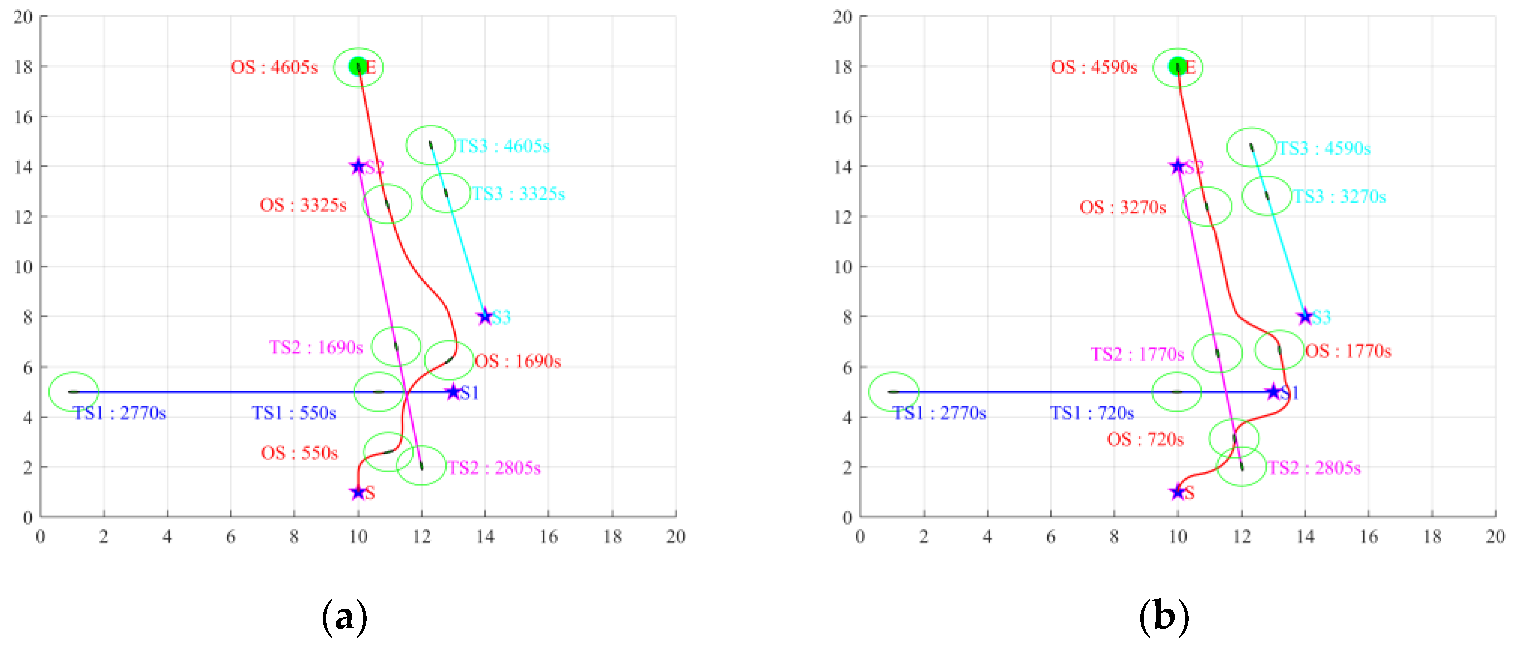
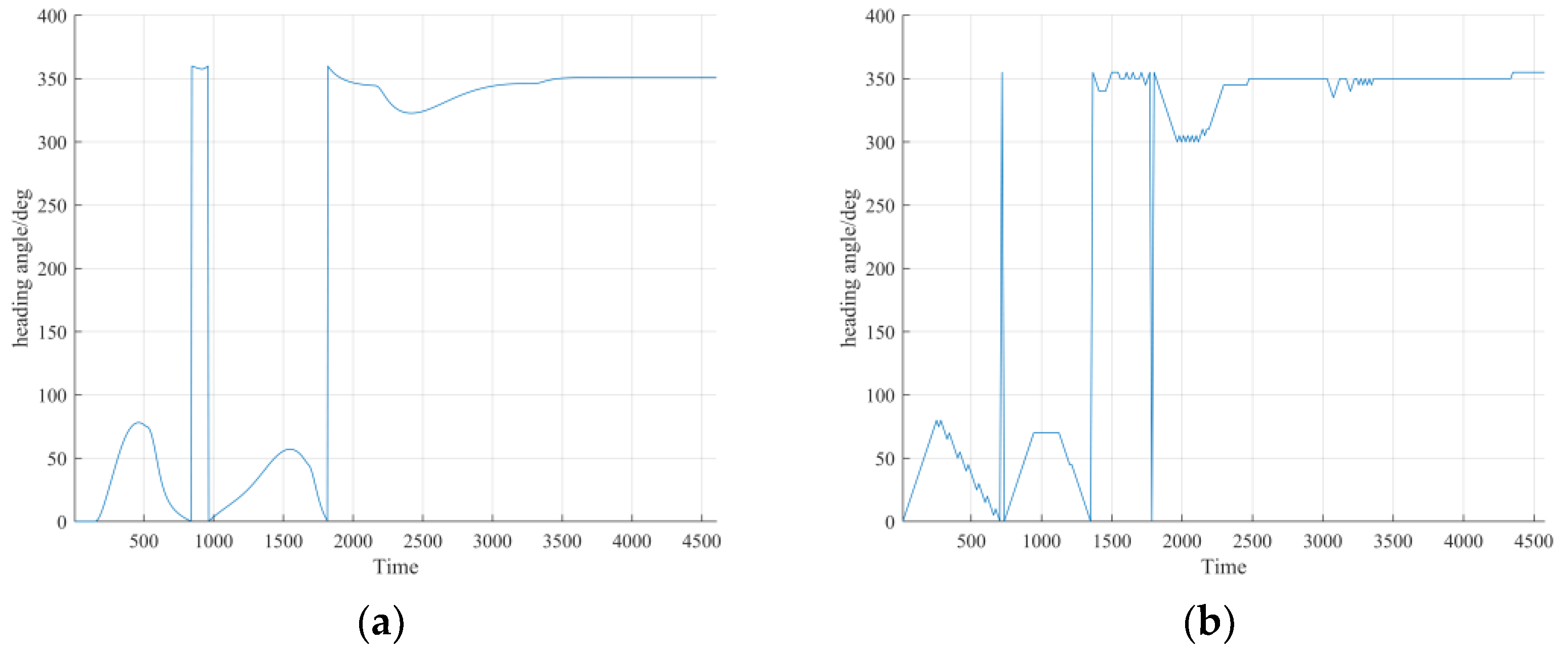
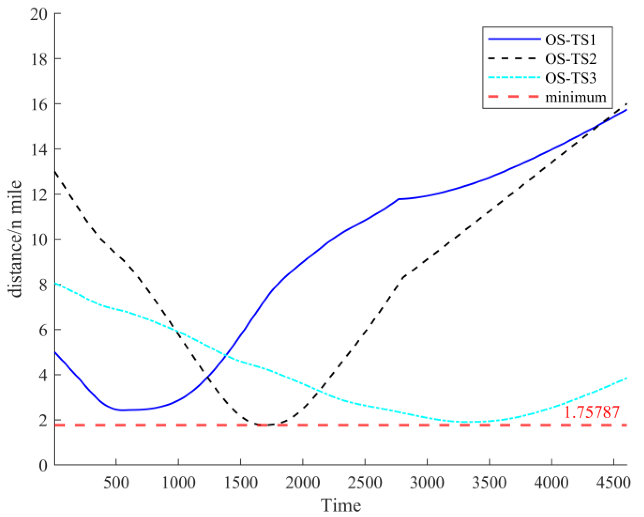
4. Simulation and Analysis

In this section, two simulations are conducted to show the effectiveness of the presented collision avoidance decision-making support scheme. Simulation 1 is a multi-ship meeting scenario where only the own ship takes action to avoid other ships. Before this, different collision avoidance action distances are set for different encounter situations between two ships, and collision avoidance actions are taken only when two ships are close to the set distance. Simulation 2 is also a multi-ship encounter scenario where the own ship considers the risk of collision with all target ships and takes appropriate actions to avoid all target ships at once. Then, the proposed scheme and an existing method [12] are simulated, respectively, under the same scenario, and the advantages of the proposed scheme are analyzed based on the simulation results. The existing method, which is a COLREGs-compliant guidance strategy based on improved APF, can choose a suitable heading according to the change in the total potential field. Therefore, the heading and the trajectory obtained by the two methods are compared in the simulation.

The benchmark ship KVLCC2 tanker is selected as a sample ship from multiple meeting ships. The data of the sample ship [24] are given in

Table 1. Principal particulars of KVLCC2 tanker.

Symbol	Quantity	Symbol	Quantity
Lpp (m)	320.0	Cb	0.81
B (m)	58.0	DP (m)	9.86
d (m)	20.8	HR (m)	15.8
Displacement (m3)	312,600	AR (m)	112.5
xG (m)	11.2

and

Table 2. Hydrodynamics force coefficients of sample ship.

Symbol	Quantity	Symbol	Quantity	Symbol	Quantity
$R_0^{\prime }$	0.022	$N_R^{\prime }$	−0.049	wp0	0.35
$X_{vv}^{\prime }$	−0.040	$N_{vvv}^{\prime }$	−0.030	C0	−2.1
$X_{vr}^{\prime }$	0.002	$N_{vvr}^{\prime }$	−0.294	$X_p^{\prime }$	−0.48
$X_{rr}^{\prime }$	0.011	$N_{vrr}^{\prime }$	0.055	tR	0.387
$X_{vvvv}^{\prime }$	0.771	$N_{rrr}^{\prime }$	−0.013	aH	0.312
$Y_v^{\prime }$	−0.315	$M_x^{\prime }$	0.022	$X_H^{\prime }$	−0.464
$Y_R^{\prime }$	0.083	$M_y^{\prime }$	0.223	γR ( βR < 0)	0.395
$Y_{vvv}^{\prime }$	−1.607	$J_z^{\prime }$	0.011	γR ( βR > 0)	0.640
$Y_{vvr}^{\prime }$	0.379	tp	0.220	$L_R^{\prime }$	−0.710
$Y_{vrr}^{\prime }$	−0.391	kt0	0.2931	ε	1.09
$Y_{rrr}^{\prime }$	0.008	kt1	−0.2753	κ	0.50
$N_v^{\prime }$	−0.137	kt2	−0.1385	fα	2.747

, respectively.

Simulation 1. 

In this simulation, a two-dimensional Cartesian coordinate system in nautical miles (nm) is utilized to express the position of the goal point and the ship. In the simulation studies, all ships sailed in open water with good visibility, and the initial states of the OS and the TS are shown in

Table 3. The initial state of the own ship and target ships in Simulation 1.

	Position	Course (°)	Surge Velocity (kn)	DCPA (nm)
OS	(10,01)	000	15.5
TS1	(13,05)	270	15.5	0.71
TS2	(10,14)	170	15.5	1.13
TS3	(14,08)	346	5.5	3.06

. The initial sway velocity, yaw rate and rudder angle of all ships are set as zero. To assess the collision risk, Table 3 lists the initial DCPA between the OS and the TS calculated from the ship’s initial position, course and velocity. Based on the data in Table 1, the coordinated ship domain R_c = 4.5L_max = 0.78 nm. The setting of a safe distance is closely related to the visibility conditions at sea, and the safe distance can be set to 1 nm when the visibility is good [33]. Combining the size of the ship domain, set the safe distance as d_safe = 1.6 nm in this simulation. Set different distances to take avoiding action for different encounter situations between the OS and the TS, e.g., as 6 nm for a head-on situation, as 4 nm for a crossing situation and as 3 nm for an overtaking situation. The primary simulation parameters are shown in

Table 4. The significant parameters in the simulation.

Description	Notations	Value
Reference distance in a head-on situation (nm)	d1	2
Reference distance in a crossing situation (nm)	d2	2
Reference distance in an overtaking situation (nm)	d3	2
Attractive potential field coefficient	katt	5
Repulsive potential field coefficient	krep	200
Time of each calculation step (s)	τ	5
Predictive horizon	Np	10
Control horizon	Nc	8
Steering factor	TE	2.5

.

The simulation results are shown in Figure 2, Figure 3, Figure 4, Figure 5 and Figure 6. Figure 2 shows the complete motion trajectories of four ships, indicating the position and the ship domain at the moment of closest proximity between the own ship and the other target ships. The curve represents the trajectory of the OS, and the other straight lines represent the trajectory of the TS. In addition, it can be observed that there is no collision risk between the target ships. Figure 2a shows the trajectories generated by the scheme based on the IAPF and NMPC methods, considering ship maneuverability. The trajectory in Figure 2b is generated by an existing method, ignoring ship maneuverability. Combined with the variation diagram of the own ship’s heading angle in Figure 3, it can be seen that the trajectory and the heading angle of the OS in Figure 2b and Figure 3b are not sufficiently smooth compared with those in Figure 2a and Figure 3a, and this difference is caused by whether the ship maneuverability is considered. In addition, there is an apparent course oscillation in Figure 3b caused by the sudden appearance or disappearance of the repulsive force at the edge of the TS’s potential field. NMPC will predict the potential field information for a period of time in the future and choose the path with the gradient of steepest descent in the total potential field to avoid repeated disappearance and appearance of the repulsive force; consequently, there is no course oscillation in Figure 3a. As observed in the figure, there is a crossing situation between the OS and TS1, a head-on situation between the OS and TS2 and an overtaking situation between the OS and TS3. According to the requirement of COLREGs, the OS takes an alternative course of action to avoid TS1, TS2 and TS3 in a sequence. There is no crossing of the ship domains, which shows that the collision avoidance effect is good. However, when the OS avoids TS1, it does not take into account the collision risk with TS2 and TS3, resulting in frequent steering maneuvers.

Figure 4 shows the variation in the distance between the OS and the TS. Obviously, combined with Figure 2, the minimum distance between the OS and the TS is higher than the safe distance d_safe, which reflects that the coordinated ship domain is more intuitive for evaluating the effect of collision avoidance. It can be seen from Figure 5 that the change in the rudder angle of the OS is always within the prescribed range in advance, which is also the most intuitive manifestation of ship maneuverability constraints. The variation diagrams of the OS’s surge, sway and resultant velocity are drawn in Figure 6, and it can be easily seen that the surge, sway and resultant velocity vary with the change in the rudder angle, which reflects the maneuvering characteristics of the ship.

Simulation 2. 

In this simulation, there is a risk of collision between the OS and all other ships, and there is no risk of collision between the target ships. As shown in

Table 5. The initial state of the own ship and target ships in Simulation 2.

	Position	Course (°)	Surge Velocity (kn)	DCPA (nm)
OS	(01,01)	045	15.5
TS1	(04,05)	045	5.5	0.71
TS2	(15,02)	315	14.5	0.53
TS3	(13,11)	225	15.5	1.41
TS4	(04,16)	135	8.5	1.32

, the initial states of the OS and the TS are given, as well as the initial DCPA between the OS and the TS. Here, the distance to take collision avoidance action is enlarged, so that the OS takes collision risk with all target ships into account when taking avoidance action. The repulsive potential field coefficient is set as k_rep = 800, and the other parameters and values are configured identically to those used in Simulation 1.

Figure 7 shows the complete motion trajectories of the OS and four target ships and marks the moment and the position of the closest distance between the OS and the TS. Figure 7a shows the trajectories generated by the scheme based on the IAPF and NMPC methods, considering ship maneuverability. The trajectory in Figure 7b is generated by an existing method, ignoring ship maneuverability. The own ship’s heading angle changes during collision avoidance using the two methods are described in Figure 8a,b, respectively. The reasons for the differences in the OS trajectory and heading angle in Figure 7 and Figure 8 are consistent with those mentioned in Simulation 1. Combined with the variation in the distance between the OS and the TS depicted in Figure 9, it can be seen that all target ships are successfully avoided by relying only on the OS to take actions. From the perspective of the OS’s trajectory, the OS adopts fewer course alterations to avoid multiple target ships. This suggests that increasing the distance of collision avoidance actions can simultaneously consider the collision risk with more target ships, effectively reducing the number of course alterations required by the OS. Meanwhile, as shown in the rudder angle change diagram in Figure 10, the maneuvering amplitude adopted by the OS in the collision avoidance process is also small. Figure 11 displays the variation diagrams of the OS’s surge, sway and resultant velocity, which vary with the change in the rudder angle, indicating the ship’s maneuvering characteristics.

5. Conclusions

In this paper, a collision avoidance decision-making support scheme based on an improved artificial potential field method and nonlinear model predictive control algorithm is proposed. In order to make the ship’s collision avoidance actions conform with the requirements of COLREGs, the repulsive potential fields of the ships in head-on, crossing and overtaking encounter situations are improved, respectively. Meanwhile, the coordinated ship domain is applied to the own ship and target ships simultaneously to ensure passage at a safe distance. The 3 DOF MMG model is utilized and transformed with the Runge–Kutta method to obtain the discrete-time nonlinear system, and then, the collision avoidance decision-making scheme is designed by combining the IAPF and NMPC methods. Moreover, two sets of simulation results show that the collision avoidance path planned by the proposed scheme not only complies with the requirements of COLREGs but also considers the maneuvering motion characteristics of the ship. Compared with the trajectory generated by an existing method, the trajectory obtained by the proposed scheme is smoother, and the proposed scheme overcomes the deficiency of course oscillation in traditional APF.

In addition, this paper does not consider the external disturbances and system uncertainties, which will be further studied to improve the practicability of the planned path in the future.

References

1. Chauvin, C.; Lardjane, S.; Morel, G.; Clostermann, J.P.; Langard, B. Human and organisational factors in maritime accidents: Analysis of collisions at sea using the HFACS. Accid. Anal. Prev. 2013, 59, 26–37. [Google Scholar] [CrossRef] [PubMed]
2. Huang, Y.; Chen, L.; Chen, P.; Negenborn, R.R.; Van Gelder, P.H.A.J.M. Ship collision avoidance methods: State-of-the-art. Saf. Sci. 2020, 121, 451–473. [Google Scholar] [CrossRef]
3. Ma, Y.; Zhao, Y.; Li, Z.; Yan, X.; Bi, H.; Królczyk, G. A new coverage path planning algorithm for unmanned surface mapping vehicle based on A-star based searching. Appl. Ocean Res. 2022, 123, 103163. [Google Scholar] [CrossRef]
4. Zhang, J.; Zhang, H.; Liu, J.; Wu, D.; Soares, C.G. A Two-Stage Path Planning Algorithm Based on Rapid-Exploring Random Tree for Ships Navigating in Multi-Obstacle Water Areas Considering COLREGs. J. Mar. Sci. Eng. 2022, 10, 1441. [Google Scholar] [CrossRef]
5. Chen, C.; Chen, X.Q.; Ma, F.; Zeng, X.J.; Wang, J. A knowledge-free path planning approach for smart ships based on reinforcement learning. Ocean Eng. 2019, 189, 106299. [Google Scholar] [CrossRef]
6. Khatib, O. The potential field approach and operational space formulation in robot control. In Adaptive and Learning Systems: Theory and Applications; Springer: Boston, MA, USA, 1986; pp. 367–377. [Google Scholar]
7. Pan, Z.; Zhang, C.; Xia, Y.; Xiong, H.; Shao, X. An improved artificial potential field method for path planning and formation control of the multi-UAV systems. IEEE Trans. Circuits Syst. II Express Briefs 2021, 69, 1129–1133. [Google Scholar] [CrossRef]
8. Huang, Y.; Ding, H.; Zhang, Y.; Wang, H.; Cao, D.; Xu, N.; Hu, C. A motion planning and tracking framework for autonomous vehicles based on artificial potential field elaborated resistance network approach. IEEE Trans. Ind. Electron. 2019, 67, 1376–1386. [Google Scholar] [CrossRef]
9. Lyu, H.; Yin, Y. Ship’s trajectory planning for collision avoidance at sea based on modified artificial potential field. In Proceedings of the 2017 2nd International Conference on Robotics and Automation Engineering (ICRAE), Shanghai, China, 29–31 December 2017; pp. 351–357. [Google Scholar]
10. Lazarowska, A. A discrete artificial potential field for ship trajectory planning. J. Navig. 2020, 73, 233–251. [Google Scholar] [CrossRef]
11. Lyu, H.; Yin, Y. COLREGS-constrained real-time path planning for autonomous ships using modified artificial potential fields. J. Navig. 2019, 72, 588–608. [Google Scholar] [CrossRef]
12. Han, S.; Wang, L.; Wang, Y. A COLREGs-compliant guidance strategy for an underactuated unmanned surface vehicle combining potential field with grid map. Ocean Eng. 2022, 255, 111355. [Google Scholar] [CrossRef]
13. Li, L.; Wu, D.; Huang, Y.; Yuan, Z.M. A path planning strategy unified with a COLREGS collision avoidance function based on deep reinforcement learning and artificial potential field. Appl. Ocean Res. 2021, 113, 102759. [Google Scholar] [CrossRef]
14. Ni, S.; Liu, Z.; Huang, D.; Cai, Y.; Wang, X.; Gao, S. An application-orientated anti-collision path planning algorithm for unmanned surface vehicles. Ocean Eng. 2021, 235, 109298. [Google Scholar] [CrossRef]
15. Oh, S.R.; Sun, J. Path following of underactuated marine surface vessels using line-of-sight based model predictive control. Ocean Eng. 2010, 37, 289–295. [Google Scholar] [CrossRef]
16. Liu, C.; Wang, D.; Zhang, Y.; Meng, X. Model predictive control for path following and roll stabilization of marine vessels based on neurodynamic optimization. Ocean Eng. 2020, 217, 107524. [Google Scholar] [CrossRef]
17. Liu, C. Motion Control of Unmanned Surface Vehicles Based on Model Predictive Control. Ph.D. Thesis, Wuhan University of Technology, Wuhan, China, 2017. [Google Scholar]
18. Abdelaal, M.; Fränzle, M.; Hahn, A. Nonlinear Model Predictive Control for trajectory tracking and collision avoidance of underactuated vessels with disturbances. Ocean Eng. 2018, 160, 168–180. [Google Scholar] [CrossRef]
19. Liu, C.; Hu, Q.; Wang, X.; Yin, J. Event-triggered-based nonlinear model predictive control for trajectory tracking of underactuated ship with multi-obstacle avoidance. Ocean Eng. 2022, 253, 111278. [Google Scholar] [CrossRef]
20. Fahimi, F. Non-linear model predictive formation control for groups of autonomous surface vessels. Int. J. Control 2007, 80, 1248–1259. [Google Scholar] [CrossRef]
21. He, Z.; Chu, X.; Liu, C.; Wu, W. A novel model predictive artificial potential field based ship motion planning method considering COLREGs for complex encounter scenarios. ISA Trans. 2023, 134, 58–73. [Google Scholar] [CrossRef]
22. Sutulo, S.; Guedes Soares, C. Mathematical models for simulation of manoeuvring performance of ships. In Marine Technology and Engineering; Taylor & Francis Group: London, UK, 2011; pp. 661–698. [Google Scholar]
23. Fossen, T.I. Guidance and Control of Ocean Vehicles; Wiley: Chichester, UK, 1994. [Google Scholar]
24. Yasukawa, H.; Yoshimura, Y. Introduction of MMG standard method for ship maneuvering predictions. J. Mar. Sci. Technol. 2015, 20, 37–52. [Google Scholar] [CrossRef] [Green Version]
25. Wang, X.; Liu, Z.; Li, T. Collision avoidance dynamic support model for ships meeting at a close range. J. Harbin Eng. Univ. 2021, 42, 1256–1261. [Google Scholar]
26. Wang, X. The Research on the Safety of Ship Navigation on the Open Sea Based on Ship Maneuverability. Ph.D. Thesis, Dalian Maritime University, Dalian, China, 2017. [Google Scholar]
27. Hu, L.; Naeem, W.; Rajabally, E.; Watson, G.; Mills, T.; Bhuiyan, Z.; Raeburn, C.; Salter, I.; Pekcan, C. A multiobjective optimization approach for COLREGs-compliant path planning of autonomous surface vehicles verified on networked bridge simulators. IEEE Trans. Intell. Transp. Syst. 2019, 21, 1167–1179. [Google Scholar] [CrossRef] [Green Version]
28. International Maritime Organization. International Regulations for Preventing Collisions at Sea (COLREGs). Available online: http://www.imo.org/en/About/Conventions/ListOfConventions/Pages/COLREG.aspx (accessed on 20 October 2022).
29. Fujii, Y.; Tanaka, K. Traffic capacity. J. Navig. 1971, 24, 543–552. [Google Scholar] [CrossRef]
30. Goodwin, E.M. A statistical study of ship domains. J. Navig. 1975, 28, 328–344. [Google Scholar] [CrossRef] [Green Version]
31. Zhang, W. A Research on Numerical Prediction of Ship Maneuverability in Regular Waves. Ph.D. Thesis, Shanghai Jiao Tong University, Shanghai, China, 2016. [Google Scholar]
32. Qin, S.J.; Badgwell, T.A. A survey of industrial model predictive control technology. Control Eng. Pract. 2003, 11, 733–764. [Google Scholar] [CrossRef]
33. Lisowski, J. Multistage Dynamic Optimization with Different Forms of Neural-State Constraints to Avoid Many Object Collisions Based on Radar Remote Sensing. Remote Sens. 2020, 12, 1020. [Google Scholar] [CrossRef] [Green Version]
Figure 1. Coordinate systems.
Jmse 11 01408 g001
Figure 2. Results of multi-ship, multiple encounter scenarios’ collision avoidance validation in Simulation 1: (a) result of the proposed method; (b) result of the existing method.
Jmse 11 01408 g002
Figure 3. Variation diagram of the own ship’s heading angle in Simulation 1: (a) result of the proposed method; (b) result of the existing method.
Jmse 11 01408 g003
Figure 4. Variation diagram of the distance between the own ship and target ships in Simulation 1.
Jmse 11 01408 g004
Figure 5. Variation diagram of the rudder angle of the own ship in Simulation 1.
Jmse 11 01408 g005
Figure 6. Variation diagram of the velocity of the own ship in Simulation 1.
Jmse 11 01408 g006
Figure 7. Results of multi-ship, multiple encounter scenarios‘ collision avoidance validation in Simulation 2: (a) result of the proposed method; (b) result of the existing method.
Jmse 11 01408 g007
Figure 8. Variation diagram of the own ship’s heading angle in Simulation 2: (a) result of the proposed method; (b) result of the existing method.
Jmse 11 01408 g008
Figure 9. Variation diagram of the distance between the own ship and target ships in Simulation 2.
Jmse 11 01408 g009
Figure 10. Variation diagram of the rudder angle of the own ship in Simulation 2.
Jmse 11 01408 g010
Figure 11. Variation diagram of the velocity of the own ship in Simulation 2.
Jmse 11 01408 g011