Abstract
Disruptions often happen to ports and cause varying degrees of port congestion. This study employs a queueing model to investigate network disruption and the resultant ripple effects in the global transportation system. We first propose an algorithm to solve the queueing model. Based on the queueing model, we obtain analytical results or propose hypotheses regarding the mechanism under disruptions. We further conduct simulations to examine the analytical results and hypotheses. Three key findings in this study are: (1) disruptions in the small port lead to a longer round-trip time compared to those in the large port; (2) herding behavior in the transportation system causes heavier congestion and also produces more emissions; and (3) major-rare disruptions cause a longer waiting time at both the port under disruption and other ports of call in the transportation system. These insights can help operators understand the mechanism of disruptions and put in place countermeasures.
1. Introduction
In the past several years, various disruptions have happened to port operations, and severe port congestion has been observed and frequently reported in the headlines of newspapers [1]. In early 2020, the COVID-19 pandemic began to spread rapidly in China, leading to labor shortages and reduced port capacity and causing significant disruptions to Chinese ports [2]; in March 2022, Shanghai implemented a lockdown to control the spread of COVID-19, which caused a large amount of congestion in Shanghai Port, the world’s busiest container port. According to UNCTAD [3], the impact of COVID-19 on the maritime industry has even surpassed that of the economic crisis in 2008. Without any doubt, COVID-19 has caused much disruption in the global supply chain as the backbone of the global supply chain—maritime transport—has suffered from many disruptions. Fortunately, the maritime industry has experienced a recovery as the COVID-19 pandemic has gradually come to an end. However, UNCTAD [4] points out that the ongoing recovery faces unprecedented port congestion, still exerting a significant impact on the reliability of the global supply chain.
In this study, we aim to investigate network disruption and its resultant ripple effects when the global transportation system is under disruption. Specifically, we conduct our analysis within three distinct contexts.
First, disruption at one port has a ripple effect on other ports and the overall transportation network [5]. As vessels travel among the network according to certain shipping routes, vessels scheduled to arrive at other ports have to wait for the congestion at the current port to clear. According to He [6], as the Port of Shanghai was jammed by ships and containers, “United States (US) supply chain companies have expressed concerns about fresh chaos heading towards American ports, which are still recovering from the severe congestion and delays they suffered last year”. Within the transportation system, ports exhibit varying service levels. Some big ports are equipped with advanced automation technology, thereby owning a high degree of service level. This motivates us to study our first research question: Suppose the same scale of disruption happens to the transportation network, which one affects the system more seriously? Does it happen to a port with a fast service speed or a port with a slow service speed?
Second, when facing disruptions in the transportation system, vessels may take a speed-up measure by arriving at their ports of call earlier with the goal of being served earlier. The transportation system may exhibit herding behavior in the presence of disruptions. That is, all vessels speed up on their shipping route and want to meet the demands faster. We wonder whether the speed-up strategy can bring the equivalent time savings in the total round-trip time. As sailing with high speed generates more fuel consumption, the speed-up strategy is not environmentally friendly. Therefore, it may be a lose-lose strategy. It prompts us to investigate the second research question: Is speed-up a good strategy when the transportation system is subject to disruptions?
Third, disruptions have different scales and occur in different frequencies. Some are large-scale, widespread, and long-lasting disruptions with rare happening probability. This type of disruption can cause serious slowdowns in port operations. For example, COVID-19 caused a large number of disruptions in the global transportation system [7,8]. According to [6], delays in shipments between China and major ports in the US and Europe have experienced a fourfold increase since the closure of Shanghai Port, the world’s busiest container port. Some are small disruptions with frequent occurrences, such as labor disputes or equipment breakdowns. Though individual disruption may be relatively small, the cumulative effect of multiple disruptions can still lead to significant delays at ports. In this study, we categorize disruptions into major-rare disruption and minor-frequent disruption and our second research question is: Given that two types of disruptions occupy ports with the same percentage of usage, which type of disruption brings a larger impact on the overall transportation network?
To explore our research questions, we first set up a closed Jackson network and then provide an algorithm to recursively solve the expected waiting time by considering travel time. By studying this algorithm, we can obtain some analytical results for the above three research questions. We then set up a simulation model using Arena, which is a simulation software that is widely applied in analyzing complex systems and processes. With the simulation model, we first examine the accuracy of the proposed algorithm and then test the analytical findings of the three research questions. Since ports are widely acknowledged as pivotal nodes within the realm of international trade and transportation, investigating and understanding the disruptions and ripple effects in the global transportation network is a significant way to provide insights into port management.
1.1. Literature Review
The studies that are closely related to our research can be divided into two categories. The first category mainly focuses on analyzing port congestion and its mechanism. The second category pays attention to making optimal plans to alleviate port congestion.
1.1.1. Mechanism of Port Congestion
Ship operations face a high level of uncertainty, e.g., the uncertainty of weather conditions at sea and labor strikes at the ports of call. These uncertainties can cause vessel delays and inefficient port operations, thereby leading to port congestion. An analysis conducted on a dataset comprising 5410 ships revealed that over 40% of these vessels have experienced delays in their arrival at ports [5]. Jiang et al. [5] investigated the “knock on” effect when the disruption occurs in a certain port. By incorporating the scenarios into a Stackelberg competition framework, they found that the “knock on” effect depended on the marginal congestion costs of terminals. Nevertheless, their investigation solely presented analytical analysis and did not conduct numerical experiments to validate the derived analytical findings. Fan et al. [9] built an intermodal network flow model to analyze the spatial congestion of container imports into the US. Hu and Zhang [10] built a fluid model to explore the whiplash effect at ports when disruptions occurred during the COVID-19 pandemic. Additionally, they applied machine learning models to predict the time spent at Shanghai Port using real-world data. Several other studies also directed their focus towards the issue of port congestion stemming from COVID-19. Notably, simulation methods have garnered substantial attention from scholars within this research domain because simulation can involve the complex and dynamic nature of the transportation system comprising both ports and vessels. Lin et al. [11] used system dynamics to evaluate strategies designed for alleviating port congestion during COVID-19. Liu et al. [12] also conducted simulations based on system dynamics and they suggested implementing advanced smart regulation systems to enhance port operational efficiency and effectively alleviate port congestion. Some studies focused on evaluating the ex-post effects of port congestion [13]. For example, Gui et al. [14] developed a framework for identifying and assessing port congestion risk regarding the port congestion during COVID-19. Based on the collected real-world data, some studies delivered empirical insights or developed data-driven models to conduct predictions. For example, Steinbach [15] conducted an empirical study based on monthly trade data at the port-product level. He found that port congestion and container shortages undermined the competitiveness of U.S. businesses in foreign markets. Peng et al. [16] built a deep learning model based on AIS data of ship sailing to predict port congestion.
1.1.2. Optimal Plans for Alleviating Port Congestion
There is a stream of literature that takes optimization techniques to deliver optimal plans that can alleviate port congestion [17]. The two main issues considered in the literature are the berth allocation plan and the ship route schedule. Imai et al. [18] proposed a heuristic procedure based on the Lagrangian relaxation to dynamically allocate berths. Wang et al. [19] designed a heuristic algorithm based on column generation to address the integrated optimization challenge encompassing berth allocation, quay crane deployment, and yard storage space allocation. Zhen et al. [20] considered uncertain vessel arrival times and uncertain numbers of loading/unloading containers when allocating resources in port operations. They proposed a two-stage stochastic integer programming model to help make optimal decisions for reducing the delays at ports. In terms of ship route schedule optimization, Wang and Meng [21] took into account the uncertainty of time at sea and at port to deliver an optimal ship route schedule design. Bütün et al. [22] studied the design of a hub-and-spoke network under congestion. They developed an innovative algorithm for obtaining optimal solutions within a short time. Ksciuk et al. [23] gave a comprehensive literature review on the ship routing and scheduling problem. Readers are referred to their study for an in-depth exploration of the pertinent literature in this field.
1.1.3. Summary
By and large, port congestion is a key issue in the domain of maritime studies and the global supply chain. Since port congestion will lead to more emissions and influence the flow of goods around the world, investigating the effects caused by port disruptions is important. To the best of our knowledge, refs. [5,10] represent the sole studies concentrating on deducing analytical insights within this domain. Our study differs from their studies. First, the methodology is different. Our analysis relies on queueing theory, in contrast to the utilization of game theory by [5] and the adoption of a fluid model by [10]. Second, the research questions are different. The authors of [5] focused more on the costs caused by port congestion. The authors of [10] investigated the process of congestion dissipation and mitigation in the transportation system. Our study pays attention to how port congestion affects different ports with different service levels, whether the speed-up strategy works in the transportation system, and how major-rare disruptions and minor-frequent disruptions affect the ports. Third, we substantiate our proposed insights through a dual approach, encompassing both theoretical validation and simulation evidence. Conversely, refs. [5] only provided theoretical proofs to support their findings.
1.2. Contributions
The contributions of our study are summarized as follows.
First, we propose an algorithm to approximately calculate the waiting time in the queueing system by taking into account the travel time. The proposed algorithm is proven with high accuracy, which means that our proposal is an innovative approach to calculate the waiting time in the transportation network.
Second, we innovatively investigate three research questions within the context of port disruptions and draw innovative findings:
- We find that the impact on the efficiency of the transportation network is more substantial when the disruption takes place in a small port instead of a large port.
- The speed-up strategy under disruption is proven to be a lose-lose strategy. That is, it generates more emissions and does not achieve the goal of meeting the demand faster.
- By simulation, we show that the major-rare disruption causes longer waiting times at all ports of call compared to the minor-frequent disruption. This is because the arrival pattern of ports is changed by disruptions.
The rest of this paper is organized as follows. Section 2 builds the queueing model and develops the algorithm for solving it. Section 3 obtains insights based on queueing analysis. Section 4 examines the accuracy of the proposed algorithm. Section 5 conducts simulations and reports the results. Finally, conclusions are drawn in Section 6.
The key notations used in this study are summarized in Table 1.

Table 1.
Notations.
2. Methodology
2.1. Closed Jackson Network and Mean Value Analysis
We model the transportation network as a closed Jackson network, where a fixed number of customers are in the system and these customers move between the queueing stations based on certain routing probabilities. In contrast, an open queueing system assumes that customers arrive from outside the system and depart after receiving service. There are a total of N ports in the network, which can be considered as servers. The service time per vessel at port i follows an exponential distribution with mean . Note that we also use j to represent the port in the following. This service time can be considered as the total time of unloading and loading time for a vessel at port i. There are a total of L vessels in the system, traveling on fixed routes. To express the traveling routes, we use to express the probability of vessels traveling to port j after visiting port i. As required by a Jackson network, the traveling time of vessels between ports is ignored. We consider such travel times in our simulation model and in Section 2.3. Given L vessels in the transportation system, the mean waiting time at port i, the mean number of vessels seen by a tagged arriving vessel, and the arrival rate of vessels at port i are denoted by , , and , respectively. We use to denote the flow rate in port i. According to traffic equations (output rate must equal input rate at each port), we have , . The mean service time or regular vessel of port i is denoted by .
For the closed queueing network, we adopt mean value analysis (MVA) to find the expected waiting time for vessels at each port; see §5 of Shortle et al. [24] for detailed instructions. This method utilizes two principles and we illustrate them in our context to facilitate reading.
- The queue length observed by an arriving vessel given L vessels in the transportation system is the same as the general time queue length with vessels in this network. Based on this principle, we can then derive the expected waiting time at port i as a function of . If no disruption happens at port i, we then haveThis equation means that the arriving vessel needs to wait for vessels before it is served and then also needs to wait for an average of another time for its own service to be carried out.
- We apply Little’s law to each port to obtain the relationship between the mean queue length, arrival rate, and mean waiting time, i.e.,
The above two principles provide a way for us to calculate the expected waiting time recursively by starting with zero vessels in the system and gradually increasing the number of vessels.
One difficulty in this algorithm is the calculation of arrival rate . This can be obtained by applying Little’s law to the whole system as follows
As we have , , we can simply pick up one port k and set its and then obtain the solution for others s. These values provide relative throughput for ports and it then follows that , for all . Replacing with in Equation (3), we have
Solving this equation yields . We then have , . The expected waiting times , the arrival rates , and the mean queue lengths at ports can be solved in the Algorithm 1.
| Algorithm 1: MVA algorithm |
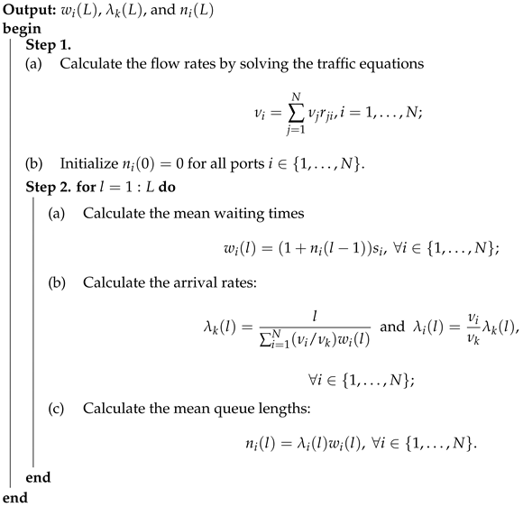 |
2.2. MVA for the Network with Disruptions
The foregoing MVA fits the network without disruptions. We now consider disruptions that happen at ports. As proposed in Ramanjaneyulu and Sarma [25], to model disruptions, we can create virtual ports and virtual vessels. For each port i, create a virtual port . There exists a virtual vessel traveling between port i and port , which represents the disruption event for port i. We use to denote the mean service time of the virtual vessel at virtual port if there is a disruption, and denotes the mean service time of the virtual vessel at port i if there is a disruption. Therefore, the usage waste of port i due to disruption is . This virtual vessel has a higher priority over regular vessels, and once it reaches port i, it preempts the vessel in service and occupies the port for an exponential time with mean , which can be considered to be the fixing time or the time for the port to resume normal operation. Once the virtual vessel leaves port i, it enters the virtual port and stays there for an exponential time with a mean . The time can be considered as the average inter-arrival time of disruptions happening to port i. Clearly, represents the usage of port i that is wasted due to disruption, or, in other words, port i is now operated with a reduced efficiency .
With this modeling approach, our transportation network now becomes a closed Jackson network with two types of customers with different priorities. Referring to Ramanjaneyulu and Sarma [25], we could use the Bryant–Krzesinski–Teunissen (BKT) approximation in Bryant et al. [26] or the Chandy–Lakshmi (CL) approximation in Chandy and Lakshmi [27] to analyze the waiting time. In this study, we adopt the CL approximation.
According to the BKT approach, we can replace the waiting time at port i in (2) with the one in an preempt resume (PR) priority queue where the disruption is considered as a preemptive high-priority customer. As well as waiting for low-priority regular vessels , the tagged vessel, upon arrival, also sees an average of virtual vessels (disruption events) in the system, which causes a delay of . Furthermore, during the stay period of the tagged vessel, there exists a chance for virtual vessels (disruption events) to arrive, which can jump up to the head of the queue and occupy the server. According to Little’s law, the expected number of virtual vessels (disruption events) arriving during the tagged vessel’s waiting time is and the delay caused by such virtual vessels (disruption events) is . Therefore, we have
From that, we can replace the waiting time expression in (2) with the following approximation obtained with an PR priority queue:
However, this approximation logic is still flawed. The key problem is that using the PR priority queue implicitly assumes that there is an infinite number of priority customers (namely, the virtual vessels) who come according to a Poisson process. However, in our port i, only one priority customer commutes between port i and the virtual port . It is possible that when a tagged vessel arrives, the virtual vessel is already in the system and hence there are no future arrivals of the virtual vessel in the following certain period of time. Hence, the BKT approximation tends to overcount the arrivals of virtual vessels.
Note that a disruption arrives only when it is located at port before arrival, which has a chance of . The CL approximation in [27] suggests to times the fraction by the disruption arrival rate in (5), leading to
The waiting time expression in (2) can then be rectified as follows
2.3. MVA for the Network with Travel Times and Disruptions
In the foregoing analysis, we assume the system to have zero travel times for vessels to commute between ports. This is clearly not realistic for the marine transportation system. Hence, we now consider how to remedy the algorithm by considering the travel times of vessels. We test our revised algorithm with simulation results.
Assume that there exists a fixed travel time for vessels to travel from port i to port j, . When travel times exist, the time for a vessel to return to a tagged port, say port i, is lengthened and hence the arrival rate to that port, namely, , becomes smaller. Denote to be the first passage time for a vessel from port i to port j, namely the time period starting from a vessel’s arrival epoch to port i, departure, and possible visiting of other ports, to its arrival epoch in port j. In particular, represents the first return time for a vessel to port i. By following the first step analysis, one can then write down the following equations for a system with L vessels.
where
Solving these equations simultaneously yields . If the system has L vessels, we can then write the arrival rate as
Hence, we can revise the MVA algorithm for the network with travel times and disruptions as follows, named the MVATD algorithm (see Algorithm 2). In Section 4, we find that, in comparison with the simulation results, the MVATD algorithm has small errors.
| Algorithm 2: MVATD algorithm |
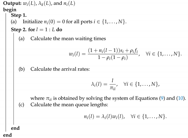 |
3. Insights Obtained via Queueing Analysis
3.1. Disruptions in Small Port Lead to Longer Round-Trip Time Compared to those in Large Port
Proposition 1.
In a transportation system with two ports (here we use t to denote the travel time between the two ports, i.e., ), port 1 is more efficient than port 2 (i.e., ). Only one port has disruption at a time, and the disruptions are stochastically the same (i.e., , , and ). The total round-trip time of a vessel is longer when a small port (i.e., port 2) is affected by a disruption than when a large port (i.e., port 1) is affected by the same scale of disruption.
Proof.
To simplify notation, we use f, , and to represent the same values of these parameters in the following. When port 1 is under disruption and , the mean waiting times at port 1 (denoted by ) and port 2 (denoted by ) are:
By the same logic, when port 2 is under disruption and , the mean waiting times at port 1 (denoted by ) and port 2 (denoted by ) are:
To investigate the round-trip time of the vessel, we need to analyze the total waiting time at two ports when port 1 is under disruption and port 2 is under the same disruption, respectively. When , the total waiting times at port 1 and port 2 under the same scale of disruption have the following relationship:
because and . Therefore, the total round-trip time of a vessel is longer when a small port is affected by a disruption than when a large port is affected by the same scale of disruption when . We define
We have because . Therefore, we can prove that
because
We also have
To simplify notation, we define , , , and . That is, we have and . Next, we prove that Equations (16), (18), and (20) hold for any L. Suppose that Equations (16), (18), and (20) hold for an , i.e.,
When the total number of vessels in the transportation system is , we have
Equation (20) holds when the total number of vessels in the network equals because
when , , and . That is, we prove that for any L.
Finally, we need to prove . We have
Therefore, we need to prove the following inequality holds:
Plugging in and , we can rewrite the above inequality:
which is
As holds, the above inequality must hold. That is, for any L. □
From Proposition 1, we can conclude that the total round-trip time of a vessel is longer when a small port is affected by a disruption than when a large port is affected by the same scale of disruption. This finding implies that the impact on the efficiency of the transportation network is more substantial when the disruption takes place in a small port. This observation is rational as small ports are more susceptible to disruptions due to their limited capacity, resources, and infrastructure. Consequently, disruptions in small ports can lead to more pronounced delays, extended round-trip times, and potentially more significant disruptions to the flow of goods compared to disruptions in larger ports. Moreover, this finding holds significant implications for practitioners, emphasizing the importance of monitoring and addressing the operations of small ports when disruptions occur, despite small ports’ seemingly insignificant presence within the broader transportation network.
3.2. Herding in the Transportation System Results in Heavier Port Congestion
Proposition 2.
In a transportation system with two ports and L vessels, port 1 and port 2 are both under disruptions, and the traveling times between these two ports are denoted by and . When the vessel’s sailing speed increases in a single trip, e.g., the traveling time decreases, the total round-trip time decreases.
Proof.
We prove this proposition by contradiction. Assume, to the contrary, that the total round-trip time increases when the vessel’s sailing speed increases in a single trip. Without loss of generality, we suppose that decreases and is fixed. We use to denote the round-trip time in this transportation system. The arrival rate is:
which decreases because we assume increases. As the service rate and are fixed, the waiting time and should decrease. Because decreases and is fixed, must decrease, which contradicts our assumption. Therefore, the total round-trip time must decrease when the vessel’s sailing speed increases in a single trip. □
Corollary 1.
In a transportation system with more than two ports, the total round-trip time decreases when the vessel’s sailing speed increases in a single trip.
Corollary 2.
In a transportation system, if the vessel speeds up in a single trip, the waiting time at the port will become longer.
Proof.
From Proposition 2, we know that when the vessel speeds up in a single trip, the round-trip time decreases, which indicates that the arrival rate at the port will increase. Therefore, the waiting time at the port will become longer. □
Corollary 2 highlights the inefficiency of herding behavior in transportation systems. When all vessels attempt to speed up and reach the destination port earlier, it leads to port congestion, resulting in longer waiting times for vessels. Consequently, the time saved in sailing does not translate into equivalent time savings in the total round-trip time. This finding indicates that herding behavior can lead to reduced efficiency in the transportation system. Moreover, as a high sailing speed generates more emissions [28], the speed-up strategy is a lose-lose strategy regarding the environment and efficiency. To improve efficiency, ship operators are advised to maintain regular sailing speeds and avoid sudden adjustments that can destabilize the system without providing substantial benefits. By avoiding herding behavior and adhering to consistent sailing speeds, the transportation system can achieve more predictable and reliable operations, ensuring optimal utilization of resources and minimizing congestion-related delays.
3.3. The Ripple Effects under Disruptions
The disruption that occurs in one port will cause ripple effects to other ports in the same transportation system [5]. Consider two scenarios, one with major (i.e., is big) and rare (i.e., is big) disruptions and the other with minor (i.e., is small) and frequent (i.e., is small) disruptions. We use superscript major and minor to indicate the two systems, respectively. The two types of disruptions bring the same usage waste to port i, i.e., . What are the ripple effects caused by the major-rare disruption and the minor-frequent disruption, respectively? Regarding the waiting time at port i, the major-rare disruption will bring a longer waiting time because the service time at port i is longer in the major-rare disruption than that in the minor-frequent disruption. Does the major-rare disruption also lead to big ripple effects on other ports in the transportation system? That is, does the major-rare disruption also cause a longer waiting time at other ports in the transportation system? We have the following two contradictory opinions.
The occurrence of a major-rare disruption at port i may result in a shorter waiting time at other ports compared to a minor-frequent disruption with an equivalent level of usage waste affecting port i. This phenomenon arises from the fact that the major-rare disruption at port i leads to a higher number of vessels becoming stalled at that specific port. Consequently, this causes a decrease in the arrival rate of other ports of call within the transportation system. Under the influence of a major-rare disruption, the arrival rates of vessels at other ports are smaller than those observed during a minor-frequent disruption. Consequently, the waiting time at other ports could be shorter, indicating small ripple effects caused by the major-rare disruption. In contrast, the minor-frequent disruption affects port i with a lower magnitude at each occurrence but may result in a more widespread and large effect across other ports. By and large, the presence of major-rare disruptions can lead to a localized impact on waiting times at other ports, potentially generating smaller ripple effects compared to the more widespread consequences caused by minor-frequent disruptions.
However, the above discussion does not consider the impact of disruption on the arrival pattern of other ports of call in the transportation system. Vessels that experience congestion at port i may subsequently converge towards downstream ports. That is, the arrival pattern in the transportation system will change. In comparison to minor-frequent disruptions, major-rare disruptions induce a more significant phenomenon of intensified vessel concentration towards downstream ports. As a result, the waiting time at other ports within the system may also experience an increase, being notably longer under the influence of major-rare disruptions in contrast to minor-frequent disruptions. That is, the ripple effects are larger under major-rare disruptions in contrast to minor-frequent disruptions.
The aforementioned contradictory viewpoints motivate us to propose the following two hypotheses and we conduct a simulation to examine which one holds in Section 5.
Hypothesis 1a.
Major-rare disruption at port i leads to a longer waiting time at port i and shorter waiting times at other ports compared to minor-frequent disruption when the two types of disruptions cause the same usage waste to port i.
Hypothesis 1b.
Major-rare disruption at port i leads to a longer waiting time at port i and longer waiting times at other ports compared to minor-frequent disruption when the two types of disruptions cause the same usage waste to port i.
4. Accuracy of the MVATD Algorithm
We now give a two-port example in this section. We need to test the accuracy of the MVATD algorithm with simulation results. We build a two-port simulation model with Arena.
Consider two ports, labeled port 1 and port 2. There are L vessels traveling between them. Ports 1 and 2 have the mean service times and , respectively. There exists a travel time of days for vessels to travel from port 1 to port 2 and time for the backward route. We create two virtual ports, port 3 and port 4. Between port 3 and port 1, there exists a virtual vessel (disruption 1) traveling between them with parameter , and between port 4 and port 2, there exists another virtual vessel (disruption 2) traveling between them with parameter . Figure 1 illustrates the transition diagram for this system. Figure 2 shows the Arena simulation model for the two-port system with independent disruptions.
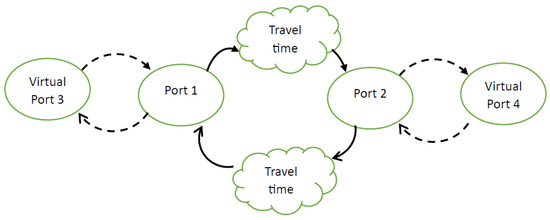
Figure 1.
State transition diagram with independent disruptions.
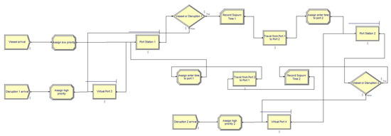
Figure 2.
Arena simulation model for two-port system with independent disruptions.
We now consider a numerical example setting for the two-port system. We set port service times to be and (https://www.econdb.com/maritime/ports/, accessed on 30 July 2023). There are nine vessels in the system. We consider travel times to be equal, i.e., , and change their values from 0 to 35 with a step length of 5.
To test the accuracy of our MVATD algorithm, we first consider a system without disruption and aim to examine whether our MVATD algorithm can correctly find the sojourn time for a network system with travel times. Table 2 illustrates the sojourn time for each port obtained from our MVATD algorithm and our simulation. We can see that they are nearly the same with a tiny difference. This experiment demonstrates that our MVATD algorithm can incorporate travel times to find the sojourn times in a queueing network.
Table 2.
Sojourn time at each port in a system without disruption.
We then consider a system with disruptions by setting and . Table 3 reports the sojourn times for each port obtained from both the MVATD algorithm and simulation. From this table, we can see that the MVATD algorithm overestimates the sojourn time and the percentage of error increases with the travel time. The percentage error with is bounded by for the slower server () and is around for the fast server (). How can we judge the MVATD algorithm’s performance according to this experiment? If we check the results of [25], we find that different algorithms for approximating the system with disruption generate outcomes with significant gaps, and the gap generated from our MVATD algorithm in comparison with the simulation result can be considered to be reasonably good. Furthermore, this performance is achieved by incorporating the travel times in the model, which is novel in the literature.
Table 3.
Sojourn time at each port in a system with disruption.
5. Simulation
5.1. Simulation Settings
In this section, we select the shipping route linking Shanghai Port (SHA) and Los Angeles Port (LA), which connects the regions of Asia and North America, as a case study for conducting simulations. SHA is the busiest container port in the world and LA stands as one of the largest ports on the western coast of the US and ranks among the busiest ports in North America [29]. These two ports suffer from disruption from time to time. For example, SHA implemented a lockdown to control the spread of COVID-19 in March 2022. In June 2023, LA suffered from a labor strike, which did not ease until the White House was involved in mediation https://www.ft.com/content/f1d67f3e-cfa5-4ddf-874c-b5a78569770a, accessed on 5 August 2023.
Referring to the statistics of CMA CGM (a container shipping company in France), we set the travel time from SHA to LA to 14 days, and the travel time from LA to SHA to 23 days https://www.cma-cgm.com/static/News/Flyers/EX1.pdf, accessed on 5 August 2023. Consistent with the setting in Section 4, and . That is, we assume the service time at SHA is 1 day and at LA is 2 days.
5.2. Results and Discussions
First, we investigate the insight introduced in Section 3.1: disruptions in a small port lead to a longer round-trip time compared to those in a large port. In our setting, SHA serves as the large port. The disruption settings are either and or and , chosen to ensure a consistent magnitude of the disruption. The results are presented in Table 4, revealing that the round-trip time during the disruption of SHA is 44.50 days, while the round-trip time during the disruption of LA is 45.71 days. This outcome aligns with the earlier theoretical deduction, demonstrating that disruptions of the same magnitude lead to longer round-trip times when the disruption occurs in a small port.
Table 4.
Round-trip time with different ports being disrupted.
Second, we examine herding in the transportation system in the scenario of SHA with a disruption ( and ). The results are reported in Table 5. Suppose the ship accelerates from SHA to LA, hoping to shorten the sailing time by half. That is, the travel time from SHA to LA is 7 days. We find that the sojourn times at SHA and LA both increase and the round-trip time is reduced by less than 7 days. That is, the time saved in sailing does not translate into equivalent time savings in the total round trip. Since speeding up also generates more emissions, herding behavior is a lose-lose strategy regarding time efficiency and environmental protection.
Table 5.
Results of herding in the transportation system.
Finally, we investigate the hypothesis introduced in Section 3.3. For the major-rare disruption, we set and ; for the major-rare disruption, we set and . The usage waste is the same. The results are shown in Table 6, and support Hypothesis 1b—major-rare disruption at port i leads to a longer waiting time at port i and longer waiting times at other ports compared to minor-frequent disruption when the two types of disruptions cause the same usage waste to port i. To test the robustness of Hypothesis 1b, we extend our analysis by varying the travel time between the two ports, ranging from 0 to 35 days in increments of 5 days. The results are shown in Figure 3. We find that the black line is always above the red line for the same port, which indicates that the major-rare disruption brings longer waiting times compared to the minor-frequent disruption. Therefore, Hypothesis 1b is supported. That is, the disruption not only affects the arrival rate of ports but also has an impact on the arrival pattern of vessels.
Table 6.
Results of major-rare disruption and minor-frequent disruption.
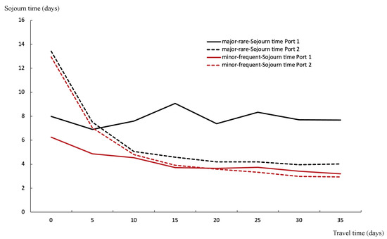
Figure 3.
Results of major-rare disruption and minor-frequent disruption with different travel times.
6. Conclusions
In this study, we investigate the network’s disruption and its resultant ripple effects when the transportation system is under disruption, e.g., COVID-19. Initially, we introduce an innovative algorithm tailored to tackle the specific queueing model pertinent to our study. Through the development of these queueing models, we derive analytical insights pertaining to the response of ports of varying sizes to disruptions of identical magnitude, as well as the manifestation of herding behavior within the transportation system. Furthermore, we extend our inquiry to encompass disruptions of differing magnitudes, culminating in the formulation of two hypotheses. Our analysis is substantiated through simulation experiments. In summation, our findings reveal that (1) disruptions in smaller ports yield longer round-trip durations in comparison to those observed in larger ports; (2) herding behavior exacerbates port congestion and contributes to increased emissions; and (3) major-rare disruptions engender prolonged waiting times not only at the directly affected port but also at other ports of call within the transportation system.
Given that disruptions exert a pervasive influence over the entire transportation system, comprehending the subsequent effects and their underlying mechanisms assumes paramount importance. This facet not only constitutes a pivotal concern but also serves as a guiding principle for operators in devising scientifically informed response strategies to effectively contend with disruptions. Since we find that disruptions in smaller ports yield longer round-trip durations in comparison to those observed in larger ports, small ports are suggested to enhance their level of automation to improve operational efficiency, thereby avoiding becoming bottlenecks in the entire transportation system when disruptions happen. Herding behavior is a lose-lose strategy, and thus, ship operators should avoid engaging in blind acceleration behavior. Major-rare disruptions have a significant impact on the entire transportation system. Adequate predictive methods are needed to monitor major-rare disruptions effectively.
Author Contributions
Conceptualization, S.G., H.W. and S.W.; methodology, S.G., H.W. and S.W.; software, S.G. and H.W.; validation, S.W.; writing—original draft preparation, S.G. and H.W.; writing—review and editing, S.W.; visualization, S.G. and H.W.; supervision, S.W. All authors have read and agreed to the published version of the manuscript.
Funding
This research received no external funding.
Institutional Review Board Statement
Not applicable.
Informed Consent Statement
Not applicable.
Data Availability Statement
Data are contained within the article.
Conflicts of Interest
The authors declare no conflict of interest.
References
- Tang, S.; Xu, S.; Gao, J.; Ma, M.; Liao, P. Effect of service priority on the integrated continuous berth allocation and quay crane assignment problem after port congestion. J. Mar. Sci. Eng. 2022, 10, 1259. [Google Scholar] [CrossRef]
- Xu, L.; Yang, Z.; Chen, J.; Zou, Z. Spatial-temporal heterogeneity of global ports resilience under Pandemic: A case study of COVID-19. Marit. Policy Manag. 2023, 1–14. [Google Scholar] [CrossRef]
- UNCTAD. COVID-19 and Maritime Transport: Impact and Responses. 2020. Available online: https://unctad.org/system/files/official-document/presspb2020d3_en.pdf (accessed on 30 July 2023).
- UNCTAD. Review of Maritime Transport. 2022. Available online: https://unctad.org/system/files/official-document/rmt2022_en.pdf (accessed on 30 July 2023).
- Jiang, C.; Wan, Y.; Zhang, A. Internalization of port congestion: Strategic effect behind shipping line delays and implications for terminal charges and investment. Marit. Policy Manag. 2017, 44, 112–130. [Google Scholar] [CrossRef]
- He, L. Shipping Delays Are Back as China’s Lockdowns Ripple around the World. 2022. Available online: https://edition.cnn.com/2022/05/06/business/china-lockdowns-global-port-chaos-supply-chains-intl-hnk/index.html (accessed on 30 July 2023).
- Xu, L.; Shi, J.; Chen, J.; Li, L. Estimating the effect of COVID-19 epidemic on shipping trade: An empirical analysis using panel data. Mar. Policy 2021, 133, 104768. [Google Scholar] [CrossRef]
- Xu, L.; Yang, S.; Chen, J.; Shi, J. The effect of COVID-19 pandemic on port performance: Evidence from China. Ocean. Coast. Manag. 2021, 209, 105660. [Google Scholar] [CrossRef] [PubMed]
- Fan, L.; Wilson, W.W.; Dahl, B. Congestion, port expansion and spatial competition for US container imports. Transp. Res. Part E Logist. Transp. Rev. 2012, 48, 1121–1136. [Google Scholar] [CrossRef]
- Hu, M.; Zhang, C. The Whiplash Effect: Congestion Dissipation and Mitigation in a Circulatory Transportation System. 2023. Available online: https://papers.ssrn.com/sol3/papers.cfm?abstract_id=4429660 (accessed on 31 August 2023).
- Lin, H.; Zeng, W.; Luo, J.; Nan, G. An analysis of port congestion alleviation strategy based on system dynamics. Ocean. Coast. Manag. 2022, 229, 106336. [Google Scholar] [CrossRef]
- Liu, J.; Wang, X.; Chen, J. Port congestion under the COVID-19 pandemic: The simulation-based countermeasures. Comput. Ind. Eng. 2023, 183, 109474. [Google Scholar] [CrossRef]
- Pengfei, Z.; Bing, H.; Haibo, K. Risk transmission and control of port-hinterland service network: From the perspective of preventive investment and government subsidies. Brodogradnja 2021, 72, 59–78. [Google Scholar] [CrossRef]
- Gui, D.; Wang, H.; Yu, M. Risk assessment of port congestion risk during the COVID-19 pandemic. J. Mar. Sci. Eng. 2022, 10, 150. [Google Scholar] [CrossRef]
- Steinbach, S. Port congestion, container shortages, and US foreign trade. Econ. Lett. 2022, 213, 110392. [Google Scholar] [CrossRef]
- Peng, W.; Bai, X.; Yang, D.; Yuen, K.F.; Wu, J. A deep learning approach for port congestion estimation and prediction. Marit. Policy Manag. 2023, 50, 835–860. [Google Scholar] [CrossRef]
- Wu, G.; Li, Y.; Jiang, C.; Wang, C.; Guo, J.; Cheng, R. Multi-vessels collision avoidance strategy for autonomous surface vehicles based on genetic algorithm in congested port environment. Brodogradnja 2022, 73, 69–91. [Google Scholar] [CrossRef]
- Imai, A.; Nishimura, E.; Papadimitriou, S. The dynamic berth allocation problem for a container port. Transp. Res. Part B Methodol. 2001, 35, 401–417. [Google Scholar] [CrossRef]
- Wang, K.; Zhen, L.; Wang, S.; Laporte, G. Column generation for the integrated berth allocation, quay crane assignment, and yard assignment problem. Transp. Sci. 2018, 52, 812–834. [Google Scholar] [CrossRef]
- Zhen, L.; Zhuge, D.; Wang, S.; Wang, K. Integrated berth and yard space allocation under uncertainty. Transp. Res. Part B Methodol. 2022, 162, 1–27. [Google Scholar] [CrossRef]
- Wang, S.; Meng, Q. Liner ship route schedule design with sea contingency time and port time uncertainty. Transp. Res. Part B Methodol. 2012, 46, 615–633. [Google Scholar] [CrossRef]
- Bütün, C.; Petrovic, S.; Muyldermans, L. The capacitated directed cycle hub location and routing problem under congestion. Eur. J. Oper. Res. 2021, 292, 714–734. [Google Scholar] [CrossRef]
- Ksciuk, J.; Kuhlemann, S.; Tierney, K.; Koberstein, A. Uncertainty in maritime ship routing and scheduling: A literature review. Eur. J. Oper. Res. 2023, 38, 499–524. [Google Scholar] [CrossRef]
- Shortle, J.F.; Thompson, J.M.; Gross, D.; Harris, C.M. Foundamentals of Queueing Theory; John Wiley & Sons: Hoboken, NJ, USA, 2018. [Google Scholar]
- Ramanjaneyulu, C.S.; Sarma, V.V.S. Modeling server-unreliability in closed queuing-networks. IEEE Trans. Reliab. 1989, 38, 90–95. [Google Scholar] [CrossRef]
- Bryant, R.M.; Krzesinski, A.E.; Teunissen, P. The MVA pre-empt resume priority approximation. In Proceedings of the ACM SIGMETRICS Conference Measurement and Modeling of Computer Systems, Minneapolis, MN, USA, 12–27 August 1983. [Google Scholar]
- Chandy, K.M.; Lakshmi, M.S. An Approximation Technique for Queuing Networks with Preemptive Priority Queues; Technical Report; Department of Computer Science, The University of Texas at Austin: Austin, TX, USA, 1983. [Google Scholar]
- Zincir, B. Slow steaming application for short-sea shipping to comply with the CII regulation. Brodogradnja 2023, 74, 21–38. [Google Scholar] [CrossRef]
- Xiao, G.; Wang, T.; Chen, X.; Zhou, L. Evaluation of ship pollutant emissions in the ports of Los Angeles and Long Beach. J. Mar. Sci. Eng. 2022, 10, 1206. [Google Scholar] [CrossRef]
Disclaimer/Publisher’s Note: The statements, opinions and data contained in all publications are solely those of the individual author(s) and contributor(s) and not of MDPI and/or the editor(s). MDPI and/or the editor(s) disclaim responsibility for any injury to people or property resulting from any ideas, methods, instructions or products referred to in the content. |
© 2023 by the authors. Licensee MDPI, Basel, Switzerland. This article is an open access article distributed under the terms and conditions of the Creative Commons Attribution (CC BY) license (https://creativecommons.org/licenses/by/4.0/).