Abstract
The significant congestion during the COVID-19 epidemic has prompted terminal managers to prioritize efforts to enhance daily operational efficiency in the post-epidemic era. In direct response to these priorities, this study develops a dynamic stack-based yard space allocation model tailored to optimize daily yard space allocation in automated container terminals. The model is based on a predeveloped yard template and considers the influence of shipping schedule fluctuations. Its primary objectives are to minimize truck movements and achieve a balanced block distribution, thereby providing theoretical support for real-time container drop-off during terminal shipping schedule fluctuations and dynamic variations in container operation flow. Through extensive experimentation, this study analyzes multiple scenarios in real automated terminal yard space management. The findings indicate that, because of bay space expansion and operational process changes, the allocation of automated terminal yard space is better suited to the stack-based processing mode. In the stack-based mode, the higher operational efficiency of automated rail-mounted gantries can help terminals achieve better dynamic allocation balances with lower energy consumption.
1. Background
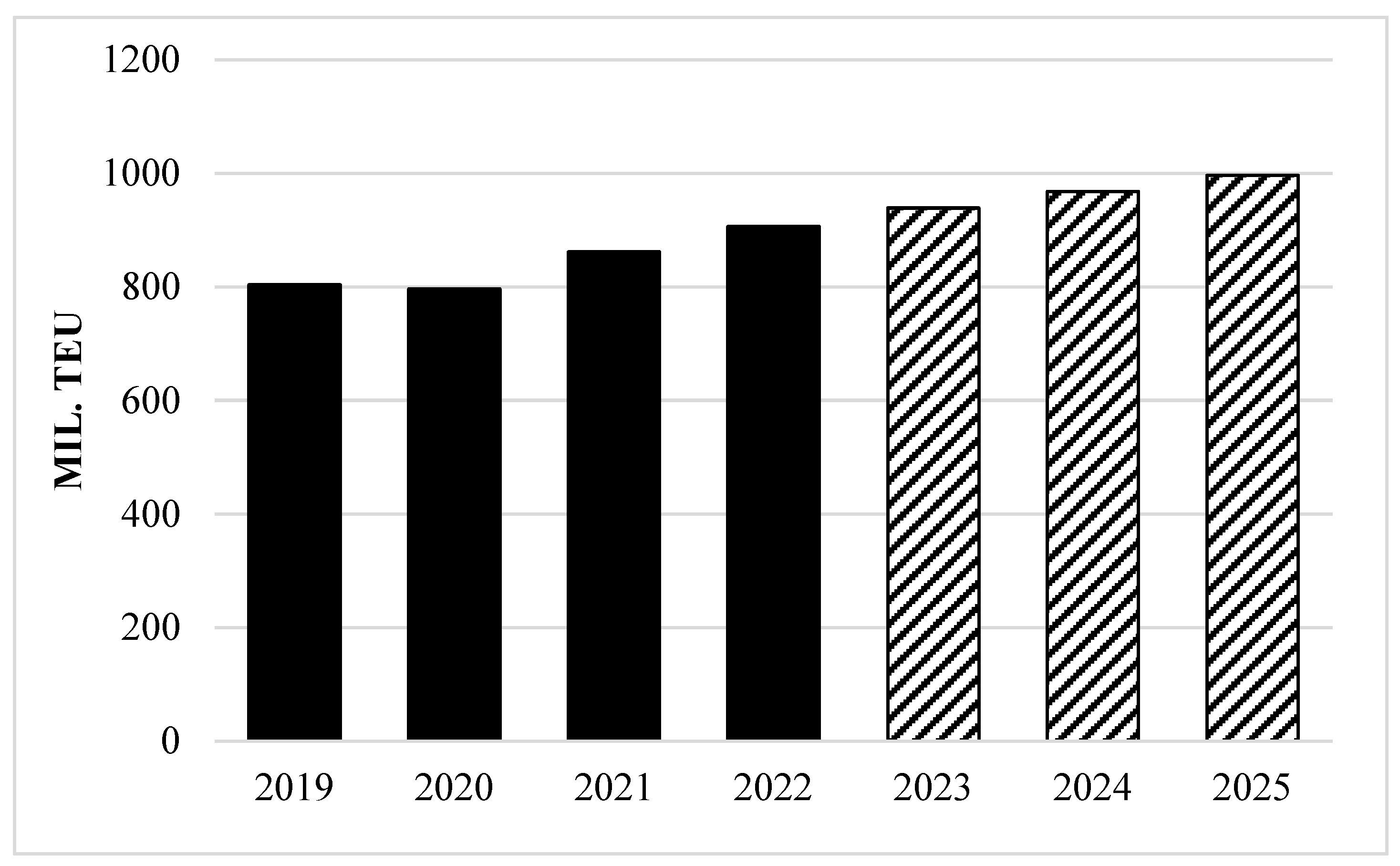
Ports serve as fundamental and vital infrastructural elements that play a crucial role in facilitating economic development. In China, ports account for more than 90% of the country’s foreign trade in cargo transportation, making port throughput a key economic indicator. According to the Drewry data statistics (as shown in Figure 1, in which the shaded columns are the forecast data), global container throughput has surpassed 800 million TEU since 2021, with China’s major ports accounting for approximately 31% of the global total. This surge in global container freight volume has spurred the demand for ultra-large container ships. Simultaneously, the berthing of these large vessels poses operational challenges for container terminals, particularly when dealing with very large ships exceeding 20,000 TEU [1].
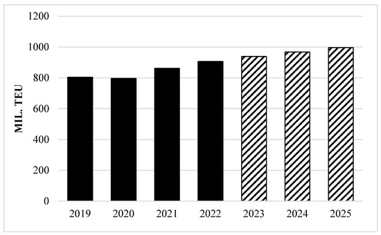
Figure 1.
Status and projections for container terminal throughput from 2019 to 2025. (Shadow for predicting data).
In recent years, major container ports worldwide have experienced varying degrees of congestion owing to the COVID-19 pandemic. This resulted in significant supply delays, cargo shortages, increased freight costs, and adverse financial implications for several companies. Consequently, there has been a growing trend in the development of container terminals to optimize processes and improve management to achieve optimal outcomes with minimal investment [2]. As container throughput continues to increase, the manual process of loading and unloading containers is prone to increasing error rates, including fatigue, operating practice violations, and human negligence, all of which are difficult to control [3]. Furthermore, the efficiency of container terminal operations is highly susceptible to unforeseen circumstances, such as the global spread of the COVID-19 pandemic. Consequently, ports are compelled to explore strategies for reducing staff numbers and enhancing operational efficiency [4]. Automation of container terminals has emerged as a prominent pathway to address these challenges [5]. The implementation of advanced intelligent automation technology offers substantial benefits in terms of reducing ports’ operational and maintenance costs and fostering innovative approaches to port development. Automated container terminals have several advantages, including high efficiency, all-weather operation, and lower labor costs [6]. Consequently, they have been extensively adopted worldwide and play a pivotal role in modern port logistics.
The development of artificial intelligence has led to rapid advancements in automated container terminals [7]. As the central system of a container terminal, the container yard plays a crucial role in coordinating its subsystems [8]. The effective allocation of yard space significantly affects the production cost, throughput, and loading/unloading efficiency of the terminal [9]. With the advancement of technology, automated container terminals are increasingly incorporating artificial intelligence and big data, making digitalization and automation inevitable future trends in yard space management [10]. The implementation of mechanical dynamic positioning technology has added to the existing advantages of automated container terminal yard space management, particularly in terms of operational cost, efficiency, and safety [11]. Enhancing the performance level of yard space management in automated container terminals is essential for improving the competitiveness of port operations in the global market. Efficient yard management can reduce energy consumption, minimize production safety risks, save manpower, and improve work efficiency and cost effectiveness [12,13,14,15]).
In the post-epidemic era, container terminals have encountered intensified competitive pressures [16]. This emphasizes the need to improve operational efficiency for sustained competitiveness. Given the yard’s critical role in terminal operations, terminal managers need to focus on optimizing yard management. Compared with traditional terminals, space management challenges in automated terminal yards exhibit distinct characteristics. The introduction of horizontal transport equipment, yard operation machinery, and yard layouts has significantly transformed container loading, unloading, and lifting processes in automated terminals. Consequently, new requirements have arisen concerning yard space management. However, existing research on terminal yards has primarily focused on traditional container terminals, neglecting the study of automated container terminal yards. Even though certain studies have addressed management strategies for automated terminals to enhance yard space utilization and operational efficiency [17], the research on automated terminal yard space management lacks systematicity. For traditional yard management, yard template generation at the tactical level is always the most important schedule. While the terminal operation system or expert decking system will guide the grounding containers to specific slots based on the template, for the automated container terminals, the import and export containers are mixed in the same block, which will reduce conflicts in operations like space shortages. As a result, the terminal operation system needs a dynamic allocation strategy at the operational level to deal with the uncertain space requirement. Hence, this study aims to conduct a comprehensive modeling of the operational-level challenges of automated terminal yard space management. The findings serve as a valuable reference for selecting daily management strategies for automated terminal yards. The next sections are organized as follows: Section 2 briefly reviews the relevant studies and points out the gap in current research. Section 3 introduces the research questions for this study. Section 4 formulates the optimization model for the container dynamic allocation, while Section 5 proposes several experiments to test the models and reveal the application of the proposed method. Furthermore, Section 6 reveals management insights for real-life operations, and Section 7 concludes the whole research.
2. Literature Review
As proposed by [18], the study has applied the VOSviewer to review the relevant research about yard management of automated container terminals in the last 20 years. Based on the review, it was concluded that research on space management in traditional terminal yards has laid the foundation for studies on space allocation in automated terminals. Ref. [19] introduced a method for enhancing yard utilization in busy transshipment ports by dynamically reserving stacking space for different liners and considering yard workload balancing to reduce traffic congestion. In ports with high workloads and limited storage capacity, ref. [20] optimized the workload distribution and implemented a strategy to stack export containers into fewer subcells, minimizing loading and unloading time. Ref. [11] integrated yard space allocation with consideration of crane deployment problems to facilitate container terminal yard decision-making, considering yard congestion and minimizing operating costs and crane movement. Furthermore, ref. [21] talked about the dispersion of container allocations, while ref. [22] talked about the choice of loading clusters.
In the dynamic allocation research on traditional terminals, ref. [23] addressed the issue of mixed stacking in container terminals. They developed a two-phase target model using a rolling planning cycle method. In the first phase, the model balances the volume of containers in each block and allocates them to respective areas using an opportunity-constrained planning approach. Subsequently, it focuses on reducing the distance trucks need to move and assigns containers to be loaded and unloaded by each ship to specific blocks. Ref. [24] studied the allocation of storage locations for export containers. They broke down this problem into two phases. In the first phase, the bays assigned to the containers of different ships are determined using a mixed-integer planning model. In the second phase, the storage location of each container is precisely determined using a mixed-sequence superposition algorithm.
In the field of automated terminal space management, researchers have drawn upon ideas from traditional terminal yard space allocation to analyze and remodel the layout and operational flow of automated terminals. Ref. [25] explored space allocation for export containers in automated container terminals. They considered the randomness of ship berthing and the collection order of export containers. They formulated an integer planning model and designed a heuristic algorithm based on simulation optimization to solve the problem. Ref. [26] examined the space allocation problem for imported containers in an automated container terminal. Their objective was to allocate yard space for incoming import containers in a manner that minimized the waiting time for automated guided vehicles (AGVs) during the space allocation process and the waiting time for external trucks during future container retrieval. They proposed an integer planning model to describe this problem. Ref. [27] focused on the allocation of space for import and export containers in automated container terminals and scheduling problems related to automated rail-mounted gantry cranes (ARMGs). They designed a novel space allocation strategy by considering safety distance constraints and exchange area capacity. Their co-optimization model aims to minimize the completion time of all storage operations and the total repetitive operation time during retrieval. They also developed a hybrid genetic algorithm based on a neighborhood search to solve the model. Ref. [28] addressed the issue of space allocation in a yard by using a single cantilevered rail-mounted gantry crane. Considering the limited stacking space in the yard, they investigated a flexible space allocation strategy. They formulated a mixed-integer quadratic programming model to minimize the cost of horizontal container transportation. This incorporated an improved particle swarm optimization algorithm.
Overall, the current research on space management for automated terminal yards has primarily focused on space allocation and equipment scheduling. Ref. [29] proposed a bay-sharing strategy and developed a two-phase mathematical model to optimize yard space allocation. In the first phase, the number of stacks allocated to each block while minimizing the shortest transport distance between the blocks and berths was determined. Workload equalization between blocks was also considered. In the second phase, the stacks were allocated to bays to minimize the transport distance for the ARMGs. Experiments conducted under various conditions and scenarios demonstrated the advantages of the bay-sharing strategy in an automated terminal. In addition, ref. [29] investigated the optimal clustering strategy for container allocation in automated container terminals. They compared the suitability of bay and stack-based yard templates for busy automated terminals and found that stack-based yard templates were more appropriate. Ref. [30] proposed a dynamic bay-based allocation method for automated container terminals. They considered the mixed stacking of import and export containers within a block and the cooperative operation between multiple yard cranes.
However, after reviewing recent studies, there are seldom discussions about dynamic yard management based on stacks for automated container terminals. As a more flexible yard template, stack-based yard generation has been proven to be more suitable for yard management of automated container terminals by previous research. As a result, the dynamic allocation of yard stacks should be further studied to improve the yard management of automated container terminals. Overall, building on these works, this study explores a dynamic stack-based allocation strategy for the mixed stacking of import and export containers in a non-cantilevered yard of an automated container terminal. The proposed dynamic yard allocation method aims to improve yard management for the stack-based template by optimizing the locations for dynamic grounding containers.
3. Problem Description
The research presented in this study focuses on space management in automated container terminals at an operational level. It operates under the assumption of a predetermined yard template with a known number of stacks assigned to each block for each ship, as the stack-based template has proven to be efficient to manage the yard space for the automated container terminals [25]. The assignment scheme for the import and export stacks is determined by considering the arrival patterns of the ships. Typically, when the terminal liners remain unchanged, frequent changes to the yard space allocation scheme are unnecessary. However, it is important to note that although the terminal liners and volume of containers loaded and unloaded by ships may not change significantly, the accuracy of ship arrival schedules cannot be guaranteed. Dynamic variations in ship arrival times arise from factors such as previous port operations and navigational influences. Hence, this study aimed to provide a dynamic allocation scheme that reflects the dynamic nature of ship arrivals.
As with conventional terminals, automated terminals must manage four types of container operations: loading export containers, unloading import containers, grounding export containers, and retrieving import containers (Figure 2). However, in automated terminals, these operations are intertwined within the same block because of the mixed storage of import and export containers. In addition, each box area has only two automatic rail gantry cranes responsible for handling these operations. Consequently, when assigning container positions, the automated terminal yard must consider the balance of operations and energy consumption between the seaport and the land. Compared with traditional container terminals, the dynamic assignment of container positions in automated terminals requires consideration of the following issues:
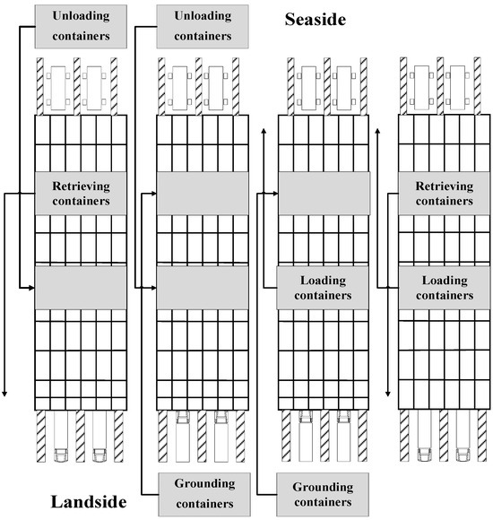
Figure 2.
Schematic diagram of the dynamic assignment of containers in an automated terminal yard.
(1) Dynamic allocation considering shipping schedule uncertainties
Once the yard space allocation scheme has been determined, conflicts arise because of the simultaneous storage of containers from different liners within the same block. Moreover, the mixing of import and export containers further complicates the operational flow. Consequently, the yard must simultaneously execute various tasks. When a bay allocation scheme is established, the automated terminal yard must devise an optimal dynamic assignment scheme to accommodate the dynamic changes in shipping schedules.
(2) Minimization of operational energy consumption when allocating containers
Real-time space allocation in an automated terminal yard requires consideration of the energy consumption of yard operation equipment. The key equipment involved in the yard space assignment typically includes AGVs and ARMGs. Terminal managers must consider the efficiency and operational energy consumption of the equipment. Consequently, the terminal should prioritize not only the yard’s operational efficiency but also the energy consumption associated with the dynamic yard space assignment.
(3) Impact of ARMG operational capabilities on allocation schemes
As mentioned previously, the operational efficiency of ARMGs is a significant bottleneck that limits the selection of yard space allocation schemes. This constitutes a crucial constraint when assigning containers. The level of the ARMGs’ activity in a specific block directly influences the workload allocated to that block. Hence, dynamic assignment must also consider the impact of the scheduling efficiency associated with ARMGs.
Ultimately, the objective of this research is to develop a dynamic container allocation model by incorporating the determined yard template and ship arrival patterns. The developed model addresses the challenge of container allocation within a specified time frame, considering fluctuations in shipping schedules. This study compares the dynamic allocation results, considering whether the overall allocation scheme was taken into account. It also analyzes the variations in energy consumption per unit for AGVs and ARMGs and examines the influence of changes in the operational capacity of ARMGs on the allocation schemes to give more inspiration for real-life yard management.
4. Model Formulation
4.1. Notation
(1) Sets and indexes
| T: | the set of time periods, indexed by t or k, ; |
| B: | the set of blocks, indexed by b, ; |
| Ω: | the set of bays, indexed by w, ; |
| Ωb: | the set of bays in block, ; |
| V: | the set of vessels, indexed by v, . |
(2) Parameters
| Qvb: | Maximum number of export container stacks belonging to the vessel stored in the block during the entire plan period; |
| Wvb: | Maximum number of import container stacks belonging to the vessel stored in the block during the entire plan period; |
| Sw: | The number of available stacks in the bay ; |
| : | The number of export containers of the vessel grounded in the time period ; |
| : | The number of import containers of the vessel unloaded in the time period ; |
| : | The number of export containers of the vessel grounded in the time period that will be loaded in the time period ; |
| : | The number of import containers of the vessel unloaded in the time period that will be retrieved in the time period ; |
| : | The number of export containers of the vessel stored in the bay before the planing that will be loaded in the time period ; |
| : | The number of import containers of the vessel stored in the bay before the planing that will be retrieved in the time period ; |
| dv,w: | The distance between the preferred berth of the vessel and the bay ; |
| : | The distance between the bay and seaside interchange point in a block; |
| lw: | The length of the block in which the bay is located, thus the distance between the bay and landside interchange point in the block is expressed as ; |
| : | Energy consumption per unit distance transported by AGVs; |
| : | Energy consumption per unit distance transported by ARMGs; |
| : | Operational efficiency of the seaside ARMG in the time period ; |
| : | Operational efficiency of the landside ARMG in the time period ; |
| : | Initial number of stacks in the block at the beginning of the decision period; |
| : | The number of containers in a stack; |
| λ: | Weights of the bi-objective function. |
(3) Decision variables
| : | The number of export stacks belonging to the vessel allocated to the bay during the time period ; |
| : | The number of export stacks belonging to the vessel allocated to the bay during the time period that will be loaded in the time period ; |
| : | The number of export stacks belonging to the vessel allocated to the bay during the time period that will be loaded outside the decision period; |
| : | The number of export stacks belonging to the vessel that will be loaded in the time period in the bay ; |
| : | The number of import stacks belonging to the vessel allocated to the bay during the time period ; |
| : | The number of import stacks belonging to the vessel allocated to the bay during the time period that will be retrieved in the time period ; |
| : | The number of import stacks belonging to the vessel allocated to the bay during the time period that will be retrieved outside the decision period; |
| : | The number of import stacks belonging to the vessel that will be retrieved in the time period in the bay; |
| : | The number of stacks stored in the bay after the time period ; |
| : | Minimum seaside operational volume in the time period ; |
| : | Maximum seaside operational volume in the time period; |
| : | Minimum landside operational volume in the time period ; |
| : | Maximum landside operational volume in the time period. |
(4) Model
Objective I: Balancing the seaside and landside workload.
Objective II: Minimizing transportation distances when allocating containers.
As mentioned earlier, the bi-objective normalization function is expressed as follows:
In Formula (3), , are the feasible solution of objectives f1 and f2, and λ is the weight of the bi-objective.
Constraints
Constraint (4) implies that the assigned export containers consist of containers to be loaded both within and outside the decision period. Constraint (5) ensures that the allocated export stacks fulfill the requirements of each vessel during each time period. Constraint (6) guarantees that the total number of stacks assigned to each bay satisfies the demand for export stacks to be loaded within that time period. Constraint (7) states that export operations within a given period encompass containers that are grounded and then loaded onto the vessel during the decision time, as well as export containers that were present in the yard prior to the decision period.
Constraint (8) specifies that the allocated import containers consist of containers to be retrieved both within and outside the decision period. Constraint (9) ensures that the allocated stacks of imported containers fulfill the assignment requirements for each vessel during each time period. Constraint (10) guarantees that the total number of stacks assigned to each bay satisfies the demand for import stacks to be retrieved within that time period. Constraint (11) states that import operations within a given period include containers that are unloaded and then retrieved during the decision period, as well as import stacks that were present in the yard before the decision period.
Constraints (12) to (17) compute the operational quantities within each block for each period, where and indicate the handling workload of seaside and landside ARMGs of block b in t, respectively. Constraints (18) and (19) guarantee that the landside and seaside operation volumes for each time window do not exceed the capacities of the corresponding landside and seaside ARMGs. Constraints (20) and (21) calculate the number of containers stored in each bay at the end of the time window to ensure that the total volume in any bay does not exceed its capacity. Constraints (22) and (23) ensure that neither incoming containers (unloaded import containers and grounded export containers) nor outgoing containers (loaded export containers and retrieved import containers) in a specific bay exceed the capacity of the bay in each time period.
4.2. Assumptions
- (1)
- The operational requirements of all vessels in this phase are known and consistent with their respective operational patterns.
- (2)
- The dynamic allocations in this phase are discussed under the assumption that the number of stacks assigned to each block for a particular ship has already been determined and the maximum number of stacks allocated to each liner in each block is known.
- (3)
- The number of stacks allocated to each bay is determined outside of the decision period.
- (4)
- No grounding or retrieval operations are permitted on the day a vessel berths.
4.3. Solution Framework
The main solution steps of the model are as follows:
| Step 1: Data initialization Step 1.1: Initialization of yard template-related data Determine the grounding requirements of export containers Determine the unloading requirements of import containers Determine the initial status of each block Step 1.2: Initialization of dynamically changing data Determine real-time changing container arrival requirements Determine real-time changing container departure requirements Step 2: Solve the model Step 2.1: Determine the boundaries of objectives f1 and f2: max f1, min f1, max f2, min f2 subject to (4)–(23) Step 2.2: Solve f by Cplex (gap < 1%). . Simultaneously, the numbers of containers loaded or retrieved inside and outside the decision making period can be obtained separately: , , , , Step 2.3: Solve the model considering global constraints Determine the boundaries of f1 and f2 for the adjusted model max f1, min f1, max f2, min f2 subject to (4)–(23) and new constraints: Solve f by Cplex (gap < 1%). , . , , , , Step 3: Yard status updates: Step 2.2 or Step 2.3 End |
Dynamic container assignment in the yard is affected by the fluctuating operations of ships within their respective time periods. Therefore, container allocation must consider the specific requirements for container operations within a given time window. The primary parameters associated with the vessel schedule for dynamic space assignment were and . Both parameters represent the key dynamic demands for grounding and unloading. Additionally, prior to the dynamic assignment, the terminal must already possess information regarding the number of grounded export containers to be loaded () and the number of unloaded import containers to be retrieved () during the subsequent decision period.
Moreover, to maintain a balanced terminal schedule and ensure stable operational efficiency throughout the yard, the number of dynamically allocated stacks must adhere to the maximum limits of the yard space allocation for export containers (Qvb) and import containers (Wvb), as illustrated below:
Constraints (24) and (25) guarantee that, for any ship during any time window, the cumulative number of assignments in each bay within any block adheres to the space allocation restrictions. This constraint emphasizes the need to consider the overall block space allocation scheme when assigning blocks within each time window.
This study utilized the Python programming language for coding. The calculations were performed on an AMD Ryzen 5 4600H@3000 Mhz platform. All the experiment cases are designed based on real-life operations and solved within acceptable time.
5. Numerical Experiments
5.1. Instance Generation
The provided calculation example focuses on determining the stack allocation scheme within the yard and assumes that the allocation of stacks in each block has already been determined. This study examined the dynamic space assignment in a block for a three-day time window. Table 1 and Table 2 present the export and import demands for each ship over the three days, where the inbound demand means there are inbounding containers for the yard during these time periods. The tables reveal the distinct characteristics of the arrival patterns of export and import containers. The export containers are collected at the harbor one day prior to the vessel’s arrival. By contrast, the import containers are unloaded upon the vessel’s arrival and leave the port based on booking arrangements. The allocation of export (Qvb) and import (Wvb) containers for each vessel within the yard templates was planned according to Table 3 and Table 4.

Table 1.
Inbound demand for export containers during the cut-off time window (stacks/day).
Table 2.
Inbound demand for import containers during the cut-off time window (stacks/day).
Table 3.
Template capacity for the export containers of each ship.
Table 4.
Template capacity for the import containers of each ship.
According to Assumption 3, the study can determine the loading and unloading operations of each container three days before the decision period; thus, the initial status of each block can be derived before the beginning of the decision period of the phase. These results are listed in Table 5 and Table 6, respectively.
Table 5.
Initial container volume distribution for blocks 1–18 in their first 12 bays.
Table 6.
Initial container volume distribution for blocks 1–18 in bays 13–26.
In addition, it should be noted that the dynamic assignment also needs to consider the specific status of the containers entering the yard within this decision period. The incoming export containers contain two parts: one to be loaded in the planning period () and the other to be loaded outside of the planning period. Import containers unloaded into the yard () also include containers to be retrieved within and outside the horizon. denotes the export containers of ship v grounded at time period t and loaded at time period t + k, and denotes the import containers of ship v unloaded at time period t and retrieved at time period t + k, the distribution of which is given in Table 7 and Table 8.
Table 7.
The number of export containers grounded and loaded during the horizon.
Table 8.
The number of import containers unloaded and retrieved during the horizon.
Drawing on former research, other relevant parameters were set as follows: the operating efficiency of a single ARMG was 110 stacks/day with a unit energy consumption of 0.0036 kWh/m, and that of the AGVs was 0.0017 kWh/m.
5.2. Results Analysis
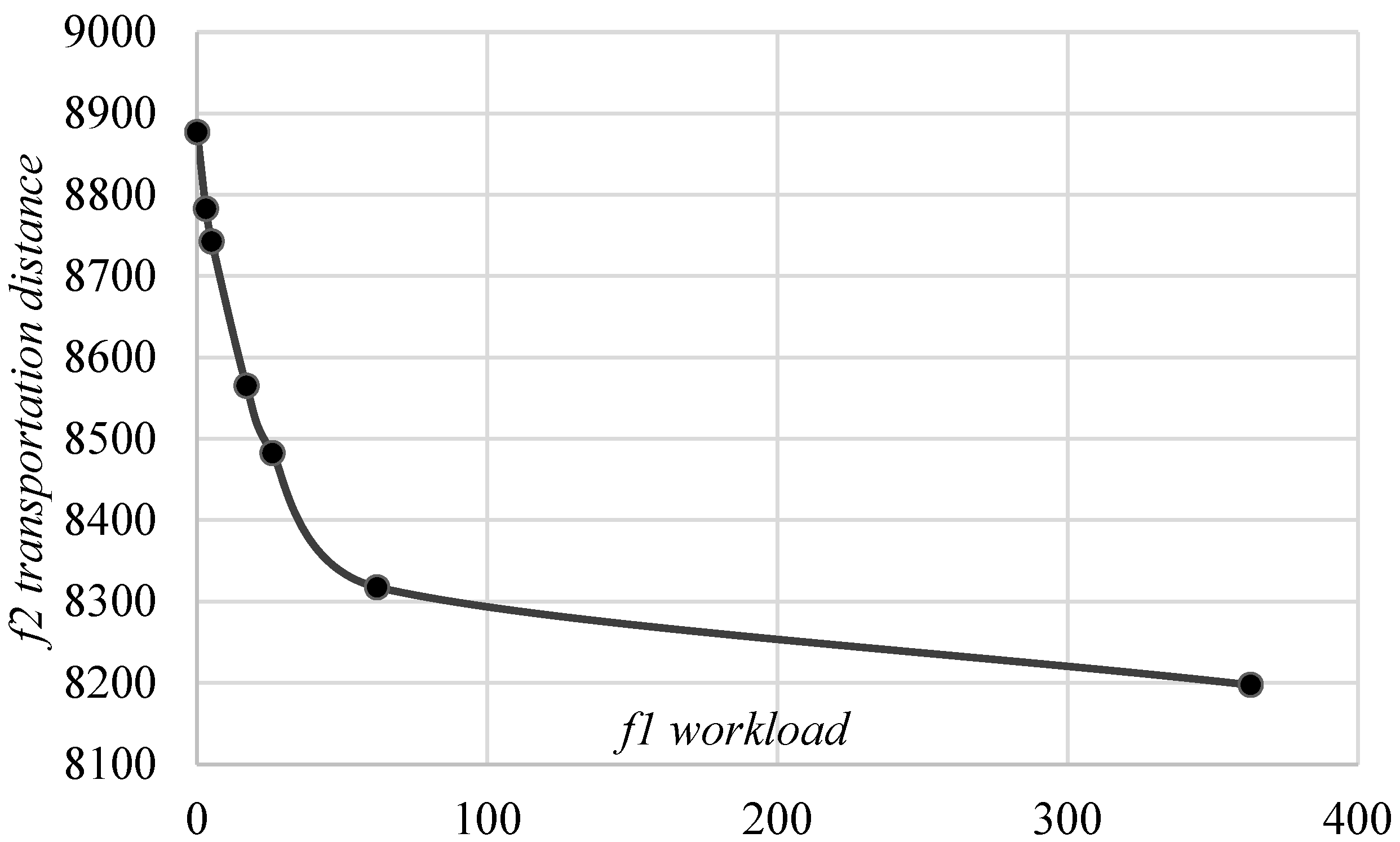
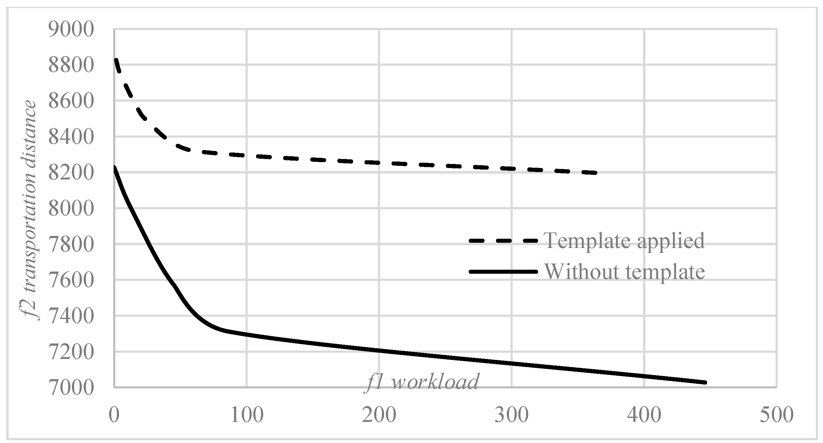
Within the aforementioned arithmetic example, the fundamental calculations of the model for this phase are depicted in Figure 3. It is evident that achieving the simultaneous minimization of transport energy consumption and operation volume equilibrium is unattainable. When the terminal aims to minimize energy consumption, container assignments tend to be concentrated, resulting in an imbalance in operation volume. Conversely, when pursuing balanced operations, it becomes challenging to ensure that containers are assigned to a block close to the preferred berth as the container space assignment becomes more dispersed. A tradeoff can be made between energy consumption (ranging from 8200 to 8300 kWh) and a balanced workload (with a difference not exceeding 60 stacks, equivalent to 300 moves).

Figure 3.
Results of dynamic allocation.
As listed in Table 9, the number of liners allocated to each block under different weights was examined. “Minimum” indicates the minimum number of liners assigned to a bay under the given weight, whereas “Maximum” indicates the maximum number of liners assigned to a bay under the same conditions. The results reveal that for each weight, the allocation of export containers requires a higher number of liners within a bay than is needed for import containers. In the management of export containers in automated terminal yards, whether at the tactical or operational level, it is crucial to consider maximizing the mixing of liners within a bay to meet terminal management requirements. However, the demand for mixed liners in import container management is relatively low. Even when the operational efficiency of an ARMG is low, import containers from multiple liners must still be included in the same bay.
Table 9.
The results of liners allocated to bays under each objective.
5.3. Scenario Analysis
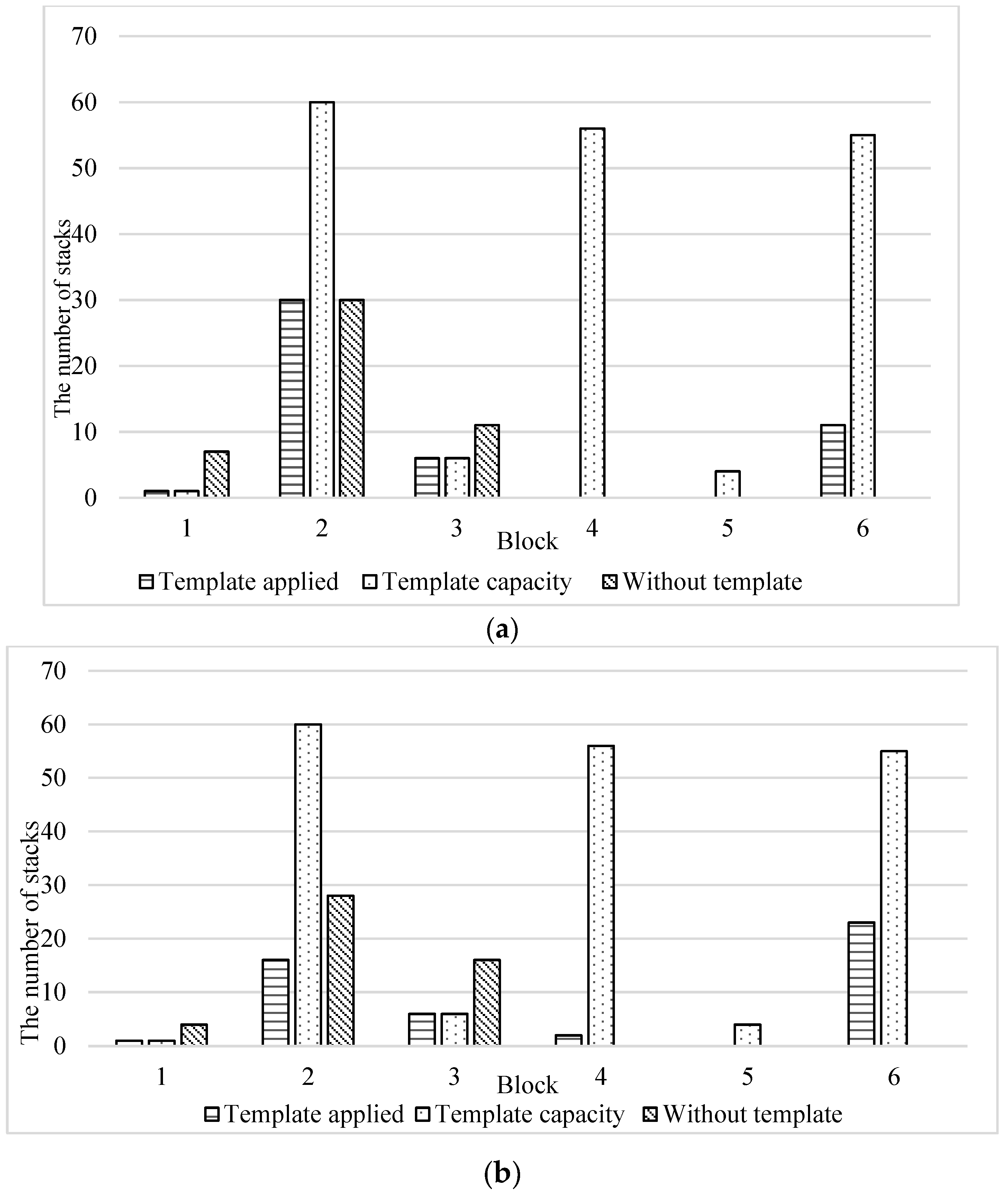
5.3.1. Comparison of Allocations with and without Yard Template Strategies
This scenario examines the outcomes of solving the model with and without considering the yard template capacity constraints. The results depicted in Figure 4 demonstrate a notable improvement in the solution when the yard template capacity constraints are not considered. This improvement stems from the greater flexibility exhibited by the solution, which disregards the yard template capacity constraints by allocating more containers. In this assignment strategy, space is allocated without considering the overall yard space allocation scheme. Instead, the focus is on achieving optimal operation within a dynamic assignment time window.

Figure 4.
Comparison of results with and without yard template constraints.
By denoting the solutions with and without consideration of the yard template capacity as VQB and V, respectively, an analysis of the containers presented at the end of each time period in each block (Table 10) highlights the distinct differences in the dynamic assignments. Solutions that do not consider the yard template capacity constraints yield completely different outcomes from those that do consider these constraints. Consequently, the operations of the containers in each bay within the same time window were significantly affected by the yard template capacity constraints.
Table 10.
Containers present after the decision time period for each block (stacks).
Upon further examination of the number of remaining stacks in the yard after the decision period (Table 11), it becomes apparent that the chosen solution objective influences the observed characteristics. When the terminal prioritizes minimizing energy consumption (smaller λ), the strategy without the yard template capacity constraints (V) tends to allocate more containers close to their future interchange points. Specifically, this is achieved by allocating more import and export containers to these favorable bays ( and will become larger), and the number of stacks remaining in the yard will be less, as shown in Table 11. Conversely, when the terminal emphasizes balancing operations (larger λ), the strategy without yard template capacity constraints tends to reduce allocation within the time window to achieve balance. By contrast, dynamic assignment that considers yard template capacity constraints (VQB) will allocate more containers to more blocks to achieve balance.
Table 11.
The number of stacks remaining in the yard under each weight (stacks).
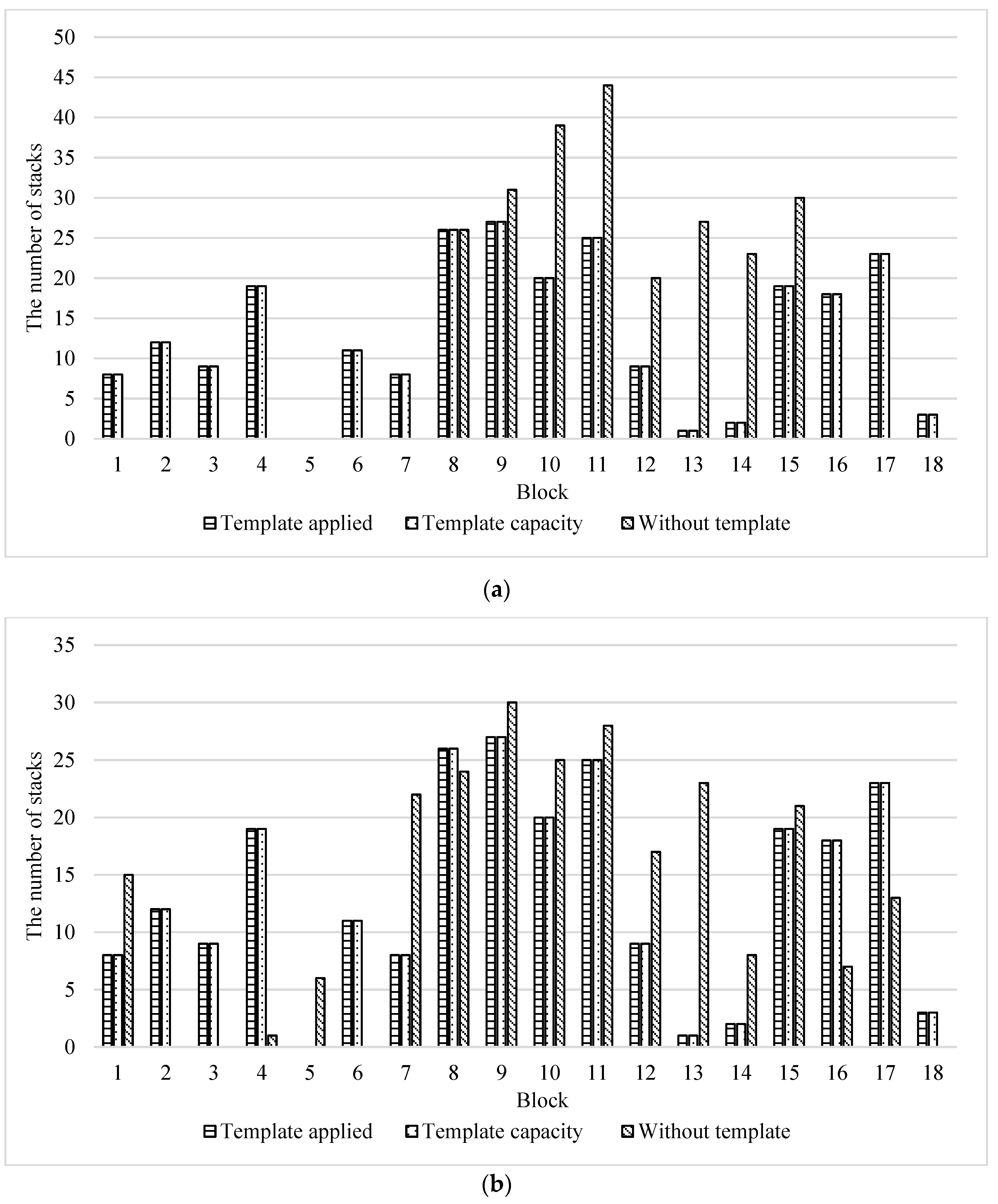
To provide a clearer representation of dynamic assignment with and without consideration of yard template capacity constraints, this study compares the assignment results under different weights (λ = 0.1 and 0.5) in Figure 5, Figure 6 and Figure 7. Figure 5 illustrates the significant differences in the assignment results when considering or disregarding yard template capacity constraints. Assignments that do not consider yard template capacity constraints demonstrate a concentrated allocation within three blocks and will surpass the capacity constraints of some blocks (e.g., blocks 1 and 3).
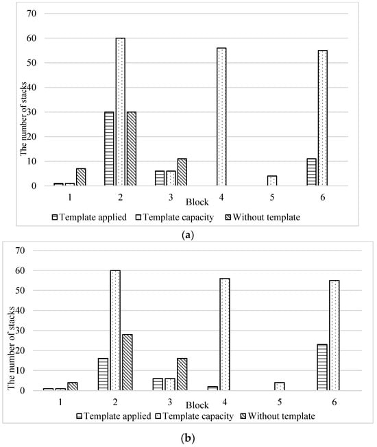
Figure 5.
Allocation of export containers of liner 1 under different weights in time period 1. (a) Results for each allocated block when λ = 0.1. (b) Results for each allocated block when λ = 0.5.

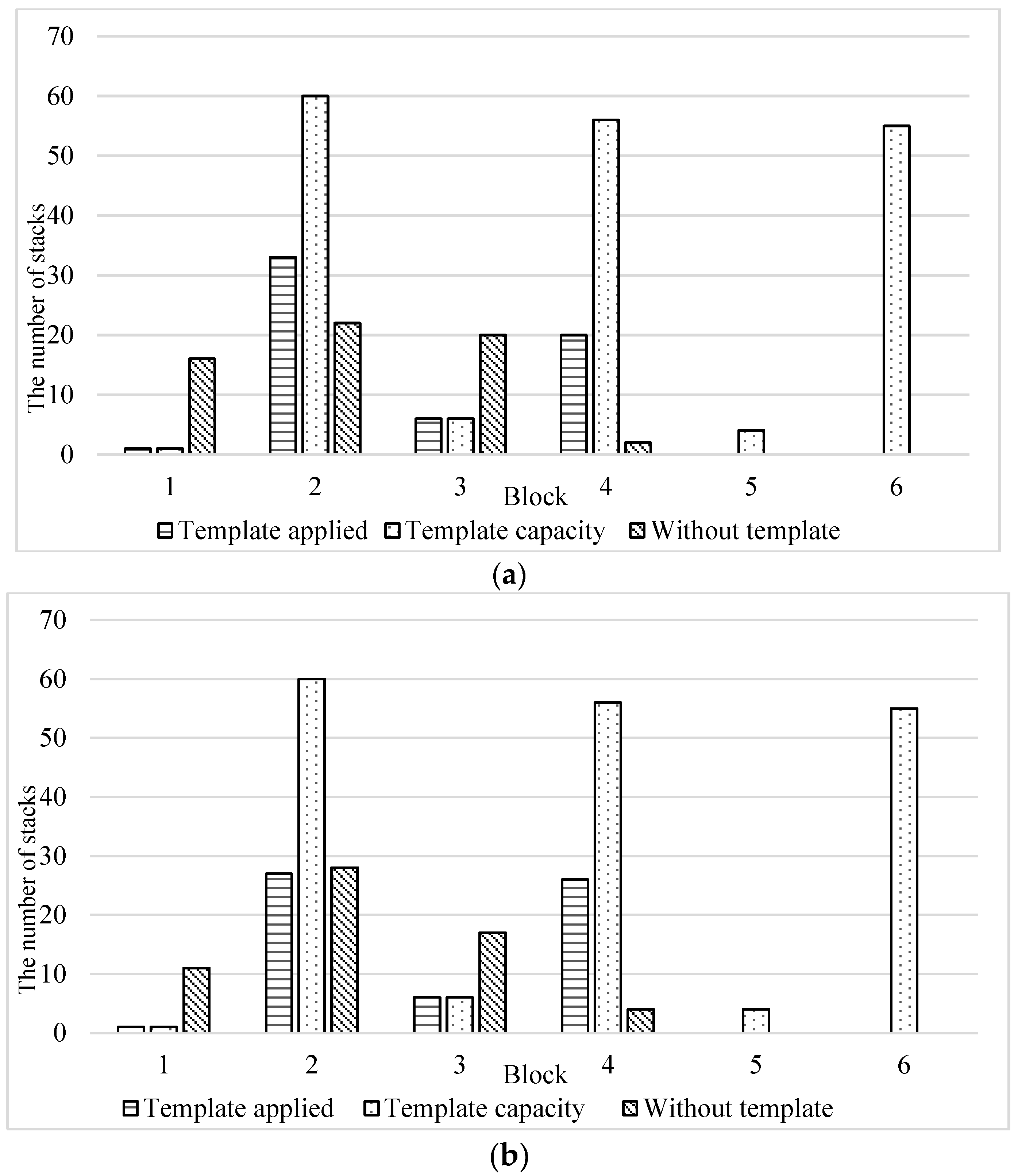
Figure 6.
Allocation of export containers of liner 1 under different weights in time period 2. (a) Results for each allocated block when λ = 0.1. (b) Results for each allocated block when λ = 0.5.
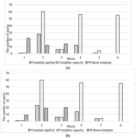
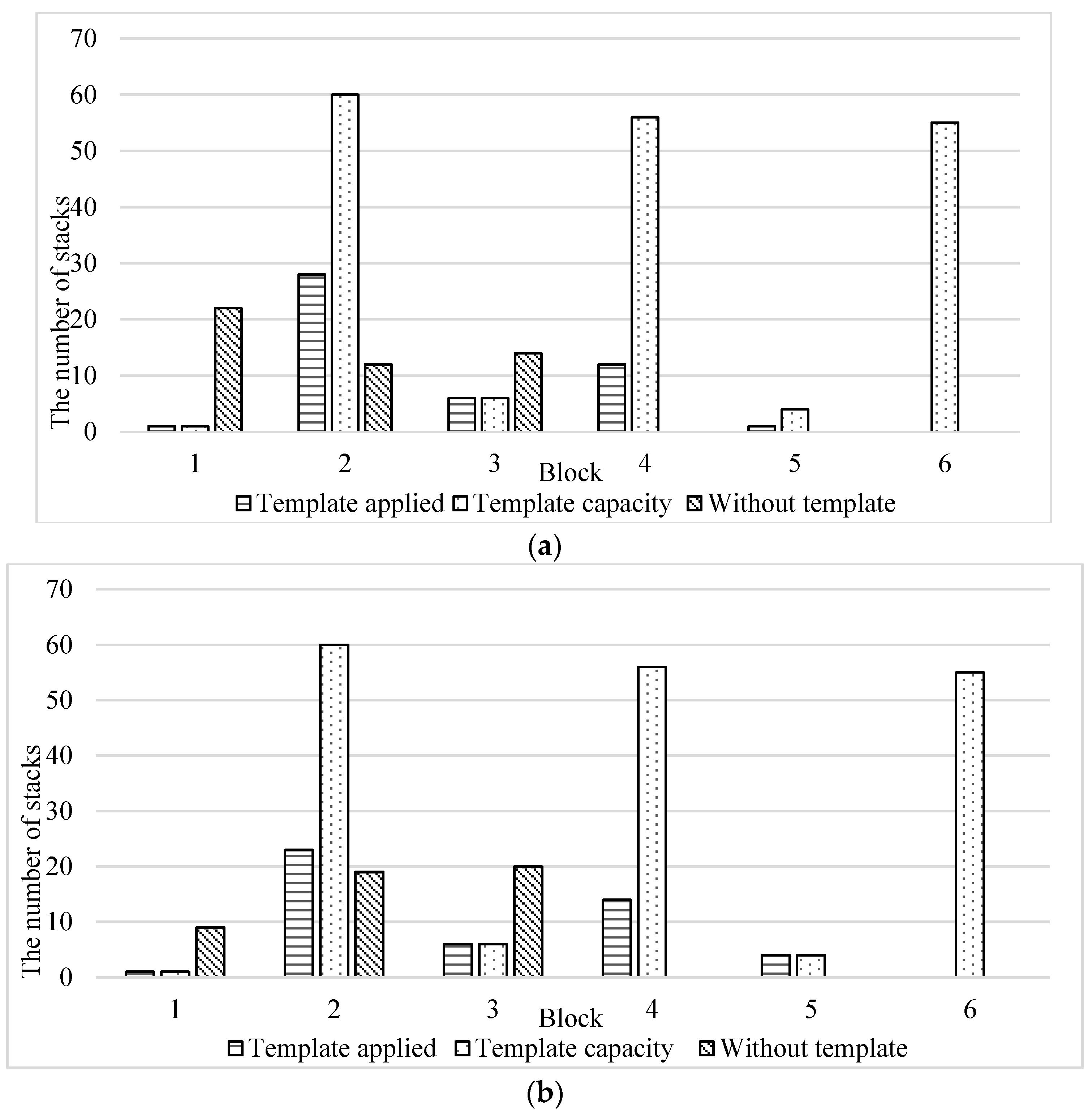
Figure 7.
Allocation of export containers of liner 1 under different weights in time period 3. (a) Results for each allocated block when λ = 0.1. (b) Results for each allocated block when λ = 0.5.
Simultaneously, as shown in Figure 6, the absence of yard template capacity constraints leads to a poorer balance in dynamic assignments as the weights increase, compared to assignments that consider yard template capacity constraints for a given liner. The model prioritizes finding the most balanced assignment method with the shortest transport distance in the absence of yard template capacity constraints, despite a stronger demand for balance. Consequently, the assignment of a liner across blocks becomes imbalanced. Furthermore, as shown in Figure 7, this study examines the assignments of liner 1 during the third time window. By synthesizing the assignments of liner 1 across multiple time windows, it becomes evident that the utilization of templates will guarantee space for the next time window. In comparison, if the terminal pursues shorter transportation distances for some time windows, the allocation without template constraints works. However, it will highly affect the space of the following container allocations.
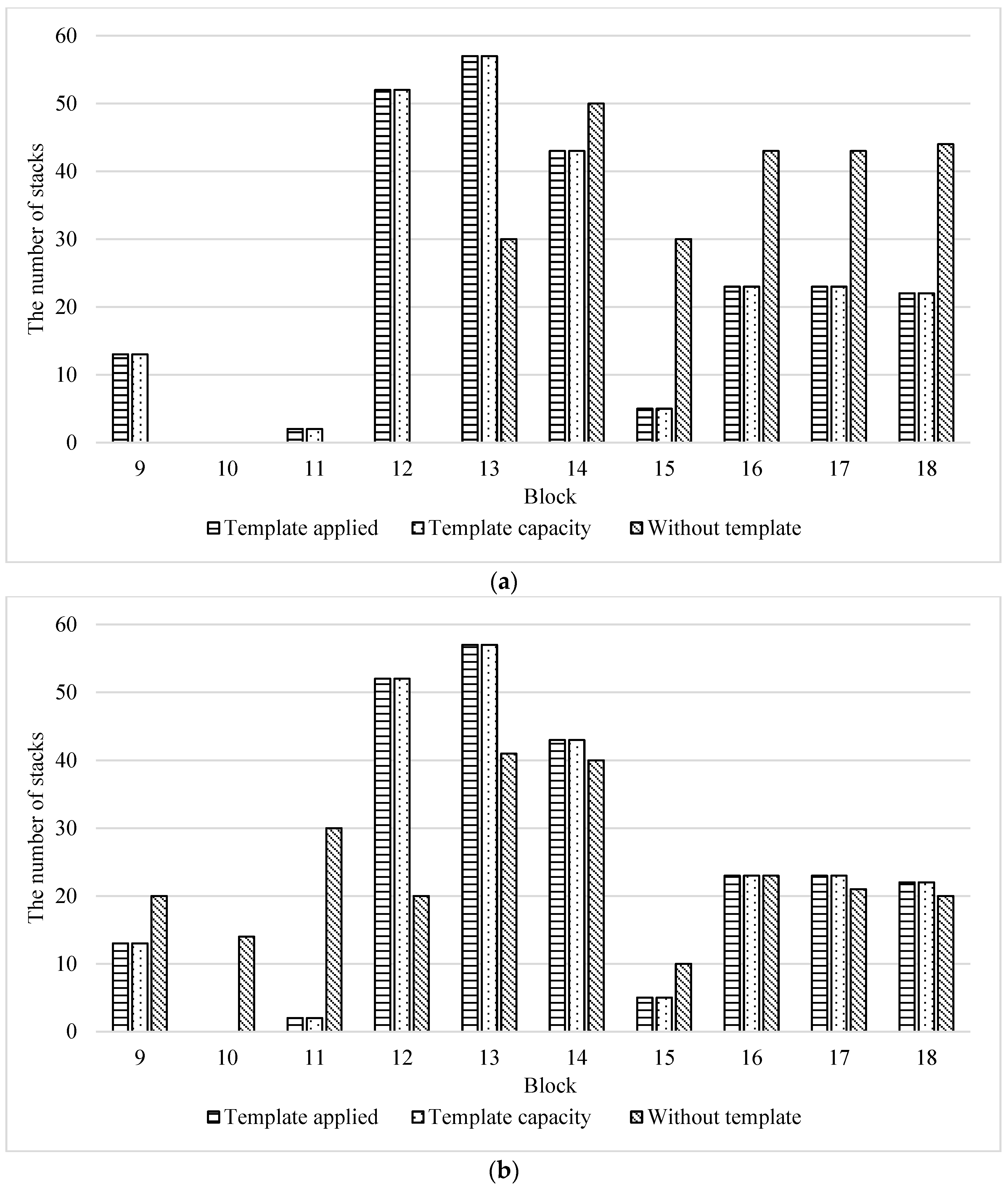
By contrast with the assignment of export containers, the assignment of import containers is more decentralized because it does not require consideration of loading efficiency and position during retrieval. This decentralized assignment approach offers advantages in terms of expediting ship unloading operations and subsequently improving the efficiency of handling imported containers by other scheduling subsystems, such as the container reservation system. The results of assigning imported containers from the different liners under various weights are shown in Figure 8, Figure 9 and Figure 10.
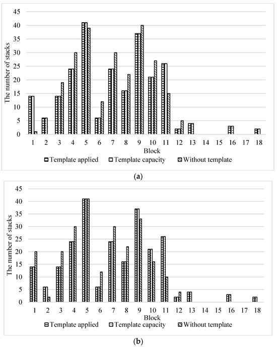
Figure 8.
Allocation of import containers of liner 1 under different weights in time period 1. (a) Results for each allocated block when λ = 0.1. (b) Results for each allocated block when λ = 0.5.

Figure 9.
Allocation of import containers of liner 1 under different weights in time period 2. (a) Results for each allocated block when λ = 0.1. (b) Results for each allocated block when λ = 0.5.
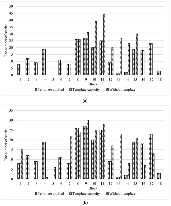
Figure 10.
Allocation of import containers of liner 1 under different weights in time period 3. (a) Results for each allocated block when λ = 0.1. (b) Results for each allocated block when λ = 0.5.
Figure 8, Figure 9 and Figure 10 demonstrate that the liner without yard template capacity constraints tends to occupy fewer blocks than the liner assigned using yard template restrictions. Moreover, the assignment distribution aligns closely with the allocation results observed under the yard template capacity constraints.
By synthesizing the assignment results of imported containers across different time windows, it is evident that a significant proportion of liners exhibit assignments that adhere to capacity constraints. This is due to the fact that the primary operational requirements for imported containers have already been considered during yard template assignment. In this container assignment phase, the focus is primarily on satisfying the unloading demand of the vessel. Therefore, assignments are made while prioritizing adherence to capacity limits and considering capacity constraint conditions whenever possible.
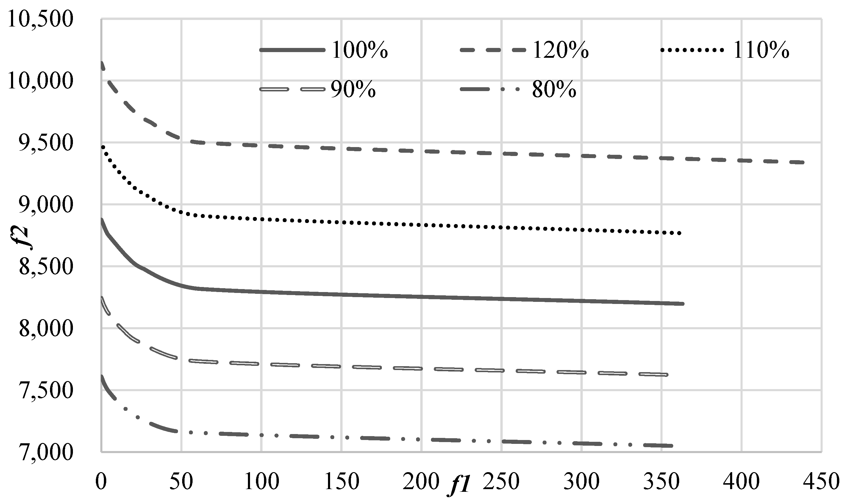
5.3.2. Impacts of Changes in Unit Energy Consumption on the Allocation
This scenario experiment focused on assessing the influence of altering the energy consumption per unit of AGVs () and ARMGs () on strategy selection. The following section presents the solution outcomes obtained by varying the unit energy consumption of AGVs and ARMGs by ±20% using the original data as the baseline scenario (100%). Figure 11 illustrates the solution results obtained by varying the energy consumption per AGV unit. The findings revealed that changes in energy consumption directly affect the lower bound of the optimal solution. Lower unit energy consumption leads to a better lower bound, and the efficiency of improvement exhibits a discernible pattern in relation to variations in unit energy consumption.

Figure 11.
Solution results when the unit energy consumption of AGVs changes.
This study presents the statistics of the minimum energy consumption under different unit energy consumption settings for AGVs, as well as the energy consumption at the most balanced time, as listed in Table 12. The findings revealed a significant decreasing trend in the minimum energy consumption as the unit energy consumption of the AGVs decreased. Moreover, the change rates of both the minimum energy consumption and the most balanced energy consumption exhibited a distinct increasing trend with decreasing unit energy consumption. This highlights the substantial effect of continuous reductions in the unit energy consumption of AGVs on the overall energy consumption during the dynamic allocation process.
Table 12.
Optimal solution performance of AGVs under fluctuations in unit energy consumption.
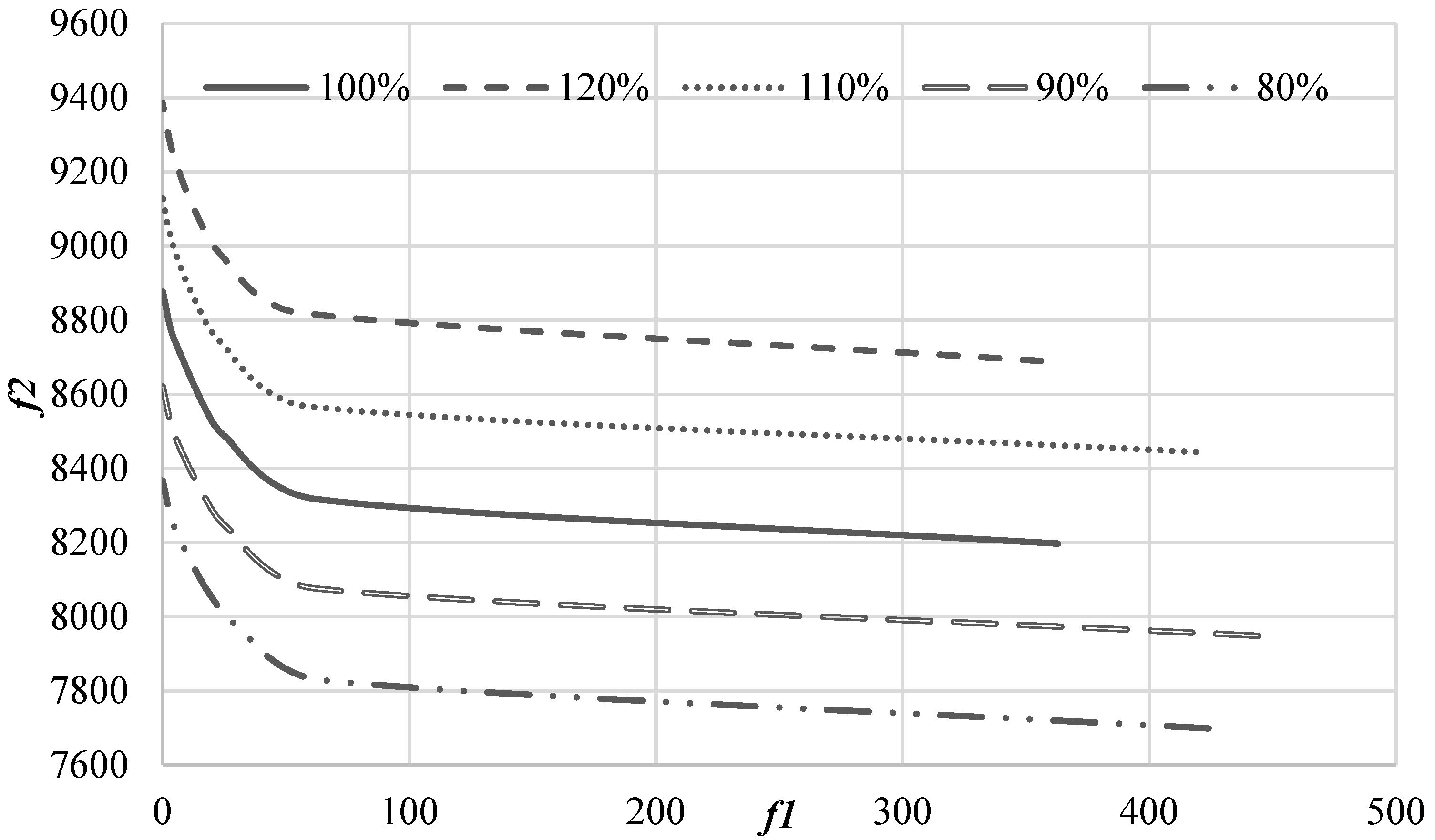
In addition, the study examined the total energy consumption when varying the unit energy consumption of the ARMGs, as illustrated in Figure 12. The variation trend in the solution is similar to that of the AGVs when the unit energy consumption was altered. However, the magnitude of the change rate in optimal energy consumption was significantly reduced for the ARMGs. As given in Table 13, even with continuous reductions in the unit energy consumption of the ARMGs, the change rate still demonstrates an increasing trend. This indicates that a continuous reduction in the unit energy consumption of the ARMGs also contributes to a reduction in the overall energy consumption during the dynamic allocation process.

Figure 12.
Solution results when the unit energy consumption of ARMGs changes.
Table 13.
Optimal solution performance of ARMGs under fluctuations in unit energy consumption.
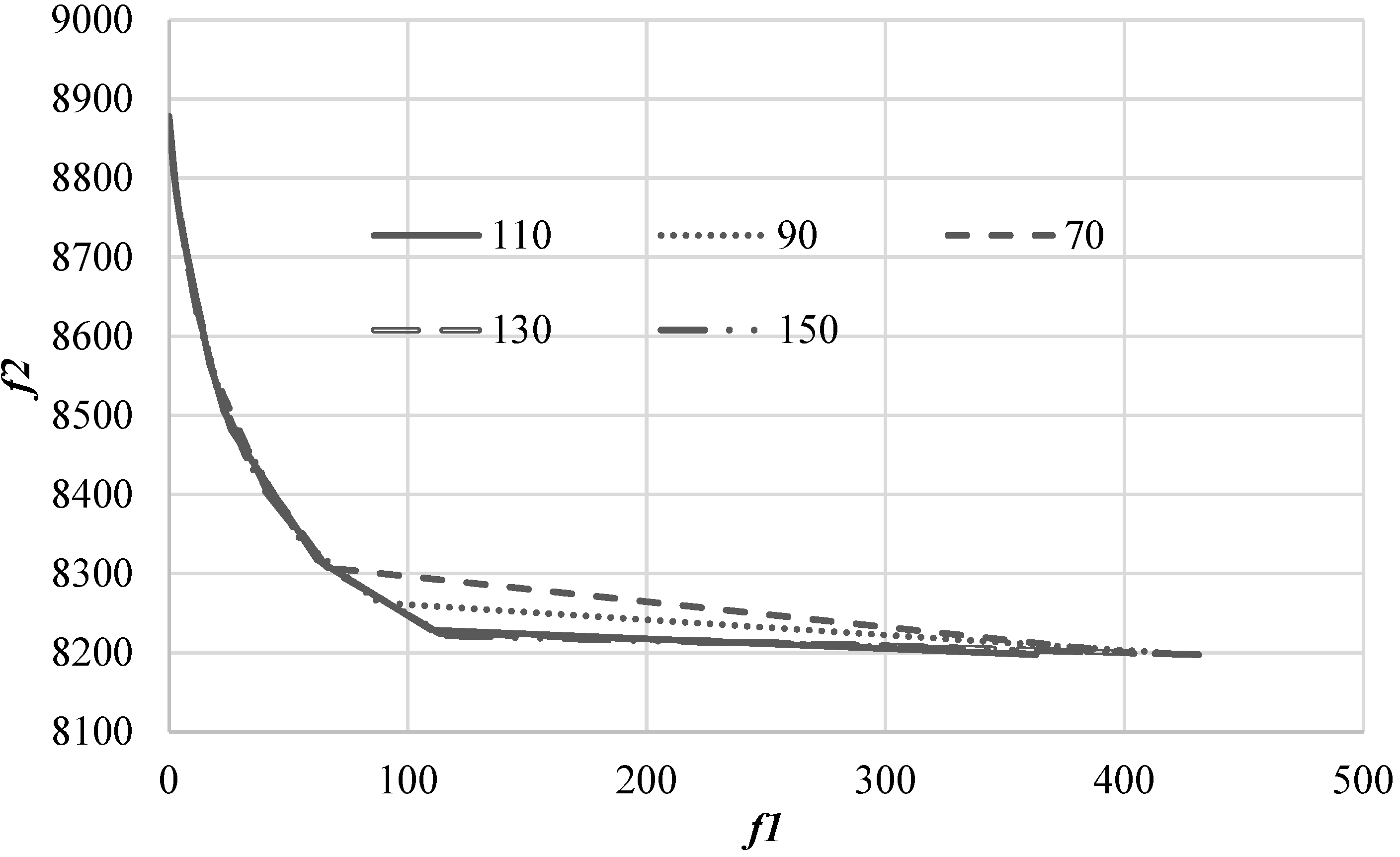
5.3.3. Comparison of Allocation Results under Changes in ARMG Efficiency
This scenario focuses on examining the influence of changes in ARMG efficiency during the dynamic allocation process. Specifically, it investigates the impact on solutions when the operational efficiencies of seaside and landside ARMGs undergo synchronous changes. The analysis was conducted by varying the ARMG efficiency from 70 to 150 stacks/day, while the baseline efficiency was maintained at 110 stacks/day. The distributions of the solutions corresponding to different ARMG efficiencies are shown in Figure 13.

Figure 13.
Solutions for ARMGs with varying efficiency.
The impact of changes in ARMG efficiency is not prominently evident in this context. This can be attributed to the constraints imposed by the yard template, which limited significant alterations in stack allocation resulting from variations in ARMG efficiency. When the efficiency of the ARMG satisfied the constraints of the space allocation scheme, the dynamic assignment within each block continued to adhere to the yard template constraints. Nevertheless, an increase in ARMG efficiency contributed to maintaining a better balance and lower energy consumption in the yard. This suggests that higher efficiency offers the terminal more options for yard space assignment, facilitating the achievement of a balance with lower energy consumption. Conversely, a reduction in ARMG efficiency limits the realization of certain assignment options.
6. Insights for Dynamic Space Allocation
Numerical experiments find that the dynamic assignment scheme constrained by the yard template does not always yield the optimal allocation scheme attainable within the yard. If the constraint on the number of stacks in each block is not considered, the obtained dynamic assignment scheme could appear advantageous in the short term but would invalidate the terminal’s yard template. In this context, the study reveals the following key observations from the examination of dynamic assignment based on the established yard template:
- Continuous improvements in the energy consumption per unit operation of AGVs and ARMGs facilitate the terminal’s ongoing reduction in total energy consumption during dynamic space assignment. Notably, reducing the unit energy consumption of the AGVs had the most significant effect on decreasing the overall energy consumption of the dynamic assignment process.
- Fluctuations in the operating efficiency of the ARMGs during dynamic assignment did not significantly alter the effect of dynamic assignment. However, these factors directly affect the dynamic assignment scheme. The higher operating efficiency of the ARMGs contributed to achieving better dynamic allocation equilibrium and lower energy consumption.
- Advantageous locations, which are bays located near the interchange points of the two sides, are of significant importance in the management of automated terminal yards. Consequently, rehandling operations play a crucial role. When time remains within a specific time window after completing the primary operations, the yard should prioritize emptying the stacks in advantageous bays through rehandling operations. This approach enhanced the real-time operational performance and overall efficiency of the yard.
The COVID-19 epidemic has markedly disrupted port operations, as evidenced by delayed vessel arrivals and port congestion, culminating in diminished operational efficiency. This situation gained the attention of terminal managers and indicated the need to improve the daily yard management, including the dynamic container allocation. As demonstrated above, even though the yard template may guide the terminal to allocate the space at the tactical level, dynamic yard repositioning and housekeeping have become more important for the daily operations. Dynamic yard management is crucial for dealing with emergency situations like epidemics or other disruptions of terminal schedules.
7. Conclusions
In the post-epidemic era, there has been a noticeable shift in focus among terminal managers towards enhancing the efficiency of daily operations. Comparing with previous research, the main contribution of this research is to propose a dynamic space assignment method based on an automated terminal yard template. Based on the preset yard template, this study modeled the dynamic space assignment over a three-day period, accounting for fluctuations in shipping schedules triggered by emergencies such as the COVID-19 epidemic. The container space assignments for import and export containers in different ship states were determined based on each ship’s arrival time. Additionally, this study investigated the impact of yard template constraints, equipment energy consumption changes, and variations in ARMG efficiency on dynamic allocation through scenario experiments. The main findings of the study, supported by the experimental results, are as follows:
- Dynamic space assignment, constrained by the yard template, does not yield an optimal allocation scheme within the yard. Ignoring the constraints may lead to a more effective short-term dynamic assignment scheme, but it invalidates the terminal’s yard template.
- Continuous improvement in the unit operational energy consumption of AGVs and ARMGs enables the terminal to consistently reduce the total energy consumption during the assignment. Notably, reducing the unit energy consumption of AGVs has a more significant impact on decreasing energy consumption during the dynamic space assignment process.
- Fluctuations in the operating efficiency of ARMGs do not significantly change the effect of dynamic space allocation but directly influence the dynamic allocation scheme. The higher operating efficiency of ARMGs contributes to lower energy consumption and improved operational balance.
Overall, the method we proposed has proven to be efficient in improving yard management by optimizing dynamic container locations. This study presents a novel dynamic space allocation model tailored to optimize terminal operations on a daily basis. This model proactively adjusts to shipping schedule variability and adheres to the terminal management strategies established by the yard template. However, uncertainty like vessel arrivals has not been modeled and further discussed in current research, which should be an important direction for future research.
Author Contributions
Methodology, L.Z.; Writing—original draft, Y.W.; Writing—review & editing, J.H.; Supervision, W.Y. All authors have read and agreed to the published version of the manuscript.
Funding
This work was supported by the National Natural Science Foundation of China [grant number 72072112, 72001135, 72002125]; the Shuguang Program of the Shanghai Education Development Foundation and the Shanghai Municipal Education Commission [grant number 22SG46]; the Natural Science Foundation of Shanghai [grant number 22ZR1426600]; the Innovation Program of the Shanghai Municipal Education Commission [grant number 2023SKZD16]; and the Shanghai Science and Technology Committee project [grant numbers 21010501800, 22010501900].
Institutional Review Board Statement
Not applicable.
Informed Consent Statement
Not applicable.
Data Availability Statement
Data is contained within the article.
Conflicts of Interest
Author Leijie Zhang was employed by the company Tianjin Port (Group) Co., Ltd. The remaining authors declare that the research was conducted in the absence of any commercial or financial relationships that could be construed as a potential conflict of interest.
References
- Xiao, G.; Yang, D.; Xu, L.; Li, J.; Jiang, Z. The application of artificial intelligence technology in shipping: A bibliometric review. J. Mar. Sci. Eng. 2024, 12, 624. [Google Scholar] [CrossRef]
- Yu, H.; Ning, J.; Wang, Y.; He, J.; Tan, C. Flexible yard management in container terminals for uncertain retrieving sequence. Ocean. Coast. Manag. 2021, 212, 105794. [Google Scholar] [CrossRef]
- Roeksukrungrueang, C.; Kusonthammrat, T.; Kunapronsujarit, N.; Aruwong, T.N.; Chivapreecha, S. An implementation of automatic container number recognition system. In Proceedings of the 2018 International Workshop on Advanced Image Technology (IWAIT), Chiang Mai, Thailand, 7–9 January 2018; pp. 1–4. [Google Scholar]
- Xiao, G.; Wang, T.; Shang, W.; Shu, Y.; Biancardo, S.A.; Jiang, Z. Exploring the factors affecting the performance of shipping companies based on a panel data model: A perspective of antitrust exemption and shipping alliances. Ocean. Coast. Manag. 2024, 253, 107162. [Google Scholar] [CrossRef]
- Kim, B.; Kim, G.; Kang, M. Study on comparing the performance of fully automated container terminals during the COVID-19 pandemic. Sustainability 2022, 14, 9415. [Google Scholar] [CrossRef]
- Schmidt, J.; Meyer-Barlag, C.; Eisel, M.; Kolbe, L.M.; Appelrath, H.J. Using battery-electric AGVs in container terminals—Assessing the potential and optimizing the economic viability. Res. Transp. Bus. Manag. 2015, 17, 99–111. [Google Scholar] [CrossRef]
- Esser, A.; Sys, C.; Vanelslander, T.; Verhetsel, A. The labour market for the port of the future. A case study for the port of Antwerp. Case Stud. Transp. Policy 2020, 8, 349–360. [Google Scholar] [CrossRef]
- Mi, W.; Yan, W.; He, J.; Chang, D. An investigation into yard allocation for outbound containers. COMPEL Int. J. Comput. Math. Electr. 2009, 28, 1442–1457. [Google Scholar] [CrossRef]
- Luo, J.; Wu, Y. Scheduling of container-handling equipment during the loading process at an automated container terminal. Comput. Ind. Eng. 2020, 149, 106848. [Google Scholar] [CrossRef]
- Wang, N.; Chang, D.; Shi, X.; Yuan, J.; Gao, Y. Analysis and design of typical automated container terminals layout considering carbon emissions. Sustainability 2019, 11, 2957. [Google Scholar] [CrossRef]
- Jin, J.G.; Lee, D.H.; Cao, J.X. Storage yard management in maritime container terminals. Transp. Sci. 2016, 50, 1300–1313. [Google Scholar] [CrossRef]
- Budiyanto, M.A.; Huzaifi, M.H.; Sirait, S.J.; Prayoga, P.H.N. Evaluation of CO2 emissions and energy use with different container terminal layouts. Sci. Rep. 2021, 11, 5476. [Google Scholar] [CrossRef]
- Sahin, B.; Soylu, A. Multi-layer, multi-segment iterative optimization for maritime supply chain operations in a dynamic fuzzy environment. IEEE Access 2020, 8, 144993–145005. [Google Scholar] [CrossRef]
- Caballini, C.; Paolucci, M. A rostering approach to minimize health risks for workers: An application to a container terminal in the Italian port of Genoa. Omega 2020, 95, 102094. [Google Scholar] [CrossRef]
- Yue, L.; Fan, H.; Ma, M. Optimizing configuration and scheduling of double 40 ft dual-trolley quay cranes and AGVs for improving container terminal services. J. Clean. Prod. 2021, 292, 126019. [Google Scholar] [CrossRef]
- Dong, G.; Liu, Z.; Lee, P.T.W.; Chi, X.; Ye, J. Port governance in the post COVID-19 pandemic era: Heterogeneous service and collusive incentive. Ocean. Coast. Manag. 2023, 232, 106427. [Google Scholar] [CrossRef]
- Covic, F. Container Handling in Automated Yard Blocks Based on Time Information. Ph.D. Thesis, University of Hamburg Systems, Hamburg, Germany, 2018. [Google Scholar]
- Yu, H.; Deng, Y.; Zhang, L.; Xiao, X.; Tan, C. Yard Operations and Management in Automated Container Terminals: A Review. Sustainability 2022, 14, 3419. [Google Scholar] [CrossRef]
- Jiang, X.; Lee, L.H.; Chew, E.P.; Han, Y.; Tan, K.C. A container yard storage strategy for improving land utilization and operation efficiency in a transshipment hub port. Eur. J. Oper. Res. 2012, 221, 64–73. [Google Scholar] [CrossRef]
- Li, M.K. Yard storage planning for minimizing handling time of export containers. Flex. Serv. Manuf. J. 2015, 27, 285–299. [Google Scholar] [CrossRef]
- Yu, H.; Ge, Y.E.; Chen, J.; Luo, L.; Liu, D.; Tan, C. Incorporating container location dispersion into evaluating GCR performance at a transhipment terminal. Marit. Policy Manag. 2018, 45, 770–786. [Google Scholar] [CrossRef]
- Yu, H.; Zhang, M.Z.; He, J.L.; Tan, C.M. Choice of loading clusters in container terminals. Adv. Eng. Inform. 2020, 46, 101190. [Google Scholar] [CrossRef]
- Wang, B. Dynamic and stochastic storage model in a container yard. Syst. Eng. Theory Pract. 2007, 4, 147–153. [Google Scholar]
- Chen, L.; Lu, Z. The storage location assignment problem for outbound containers in a maritime terminal. Int. J. Prod. Econ. 2012, 135, 73–80. [Google Scholar] [CrossRef]
- Yu, H.; Huang, M.; He, J.; Tan, C. The clustering strategy for stacks allocation in automated container terminals. Marit. Policy Manag. 2023, 50, 1102–1117. [Google Scholar] [CrossRef]
- Yu, M.; Liang, Z.; Teng, Y.; Zhang, Z.; Cong, X. The inbound container space allocation in the automated container terminals. Expert Syst. Appl. 2021, 179, 115014. [Google Scholar] [CrossRef]
- Fan, H.; Peng, W.; Ma, M.; Yue, L. Storage space allocation and twin automated stacking cranes scheduling in automated container terminals. IEEE Trans. Intell. Transp. Syst. 2021, 23, 14336–14348. [Google Scholar] [CrossRef]
- Yang, X.; Hu, H.; Cheng, C. Flexible yard space allocation plan for new type of automated container terminal equipped with unilateral-cantilever rail-mounted gantry cranes. Adv. Eng. Inform. 2023, 58, 102193. [Google Scholar] [CrossRef]
- Yu, H.; Huang, M.; Zhang, L.; Tan, C. Yard template generation for automated container terminal based on bay sharing strategy. Ann. Oper. Res. 2022, 1–19. [Google Scholar] [CrossRef]
- He, J.; Xiao, X.; Yu, H.; Zhang, Z. Dynamic yard allocation for automated container terminal. Ann. Oper. Res. 2022, 1–22. [Google Scholar] [CrossRef]


Disclaimer/Publisher’s Note: The statements, opinions and data contained in all publications are solely those of the individual author(s) and contributor(s) and not of MDPI and/or the editor(s). MDPI and/or the editor(s) disclaim responsibility for any injury to people or property resulting from any ideas, methods, instructions or products referred to in the content. |
© 2024 by the authors. Licensee MDPI, Basel, Switzerland. This article is an open access article distributed under the terms and conditions of the Creative Commons Attribution (CC BY) license (https://creativecommons.org/licenses/by/4.0/).