Improved Low-Drag Pontoons for Water Bikes

Abstract

The popularity of modern water bikes increases due to the relatively high speed developed with the use of a human muscle power only. For example, the maximum speed of prototypes reaches the value 3 m/s. Similar vehicles can be used not only for recreation and fitness, but also for transportation. To increase their speed and tonnage, we recommend improving the pontoon shape and using electrical power. The underwater part of the pontoon shape was recommended to be similar to the body shape of the fastest fish in order to decrease the wave resistance and total drag. The optimal depth of the movement of corresponding shapes was calculated. The total drag and maximum speeds of the vehicles with the human muscle and electrical power are estimated. Expected success in improving the pontoon shape opens wide prospects for the use of these special-shaped hulls in shipbuilding.

1. Introduction

A modern water bike, Explorer-1 [1], can develop speeds of up to 2.7 m/s using only human muscle power at a total weight of 240 kg. This rather high speed was achieved by improving the shape of pontoons and using an effective propeller [1]. Similar vehicles can be used not only for recreation and fitness, but also for transportation, especially with the use of electrical power. To increase the speed and the commercial effectiveness (weight-to-drag ratio) of such vehicles, special-shaped pontoons of low drag (similar to the body shape of the best swimmers) are proposed.

The maximum speed of the fastest fish can reach around 30 m/s (e.g., sailfish, swordfish, black marlin, etc., [2,3,4,5]). A very sharp nasal rostrum of these animals probably allows them to remove the boundary layer separation and avoid high pressures on the body surface as well as reduce the wave resistance when moving near the water surface. The corresponding axisymmetric bodies with concave noses have no pressure peaks on their shape and have much lower values of the vertical velocity on the water surface [6]. Since the reason for the waves on the water surface is the high pressure on the vessel bow and stern [7,8,9,10], these special-shaped bodies could be used to reduce wave resistance. Some other results concerning the optimization of the ship’s hull can be found in [11,12,13,14,15,16].

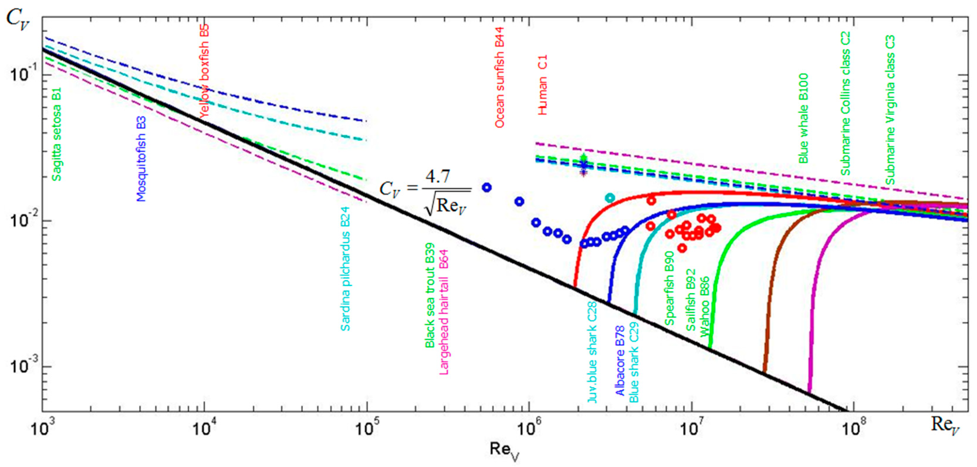
It was shown in [17] that axisymmetric bodies similar to the trunks of water animals can ensure an underwater flow pattern without boundary separation. It was proposed to use dolphin-like shapes for the underwater hulls of SWATH (Small Waterplane Area Twin Hulls) yachts and ferries [18]. The expected values of volumetric drag coefficient $C_V$ can be reduced more than twice in comparison with known shapes in the range of volumetric Reynolds numbers ${\mathrm{Re}}_V$ from 1 to 10 million (see [17], Figure 1). The corresponding volumetric coefficients can be calculated as follows:

$$C_V=\frac{2X_{}}{\rho U^2{V}_{}^{\raisebox{1ex}{$2$}\!\left/ \!\raisebox{-1ex}{$3$}\right.}}{\mathrm{Re}}_V=\frac{U_{}{V}_{}^{\raisebox{1ex}{$1$}\!\left/ \!\raisebox{-1ex}{$3$}\right.}}{\nu }$$

where V is the volume (displacement), $U$ is speed, X is the total drag, and $\rho$ and $\nu$ are the density and kinematic viscosity of water, respectively. These values of $C_V$ (shown in Figure 1 by the black solid line) are smaller than the drag on some special-shaped bodies of revolution [19,20,21] (see markers in Figure 1).

Small disturbances of the water surface caused by the special-shaped bodies of a revolution with concave noses (similar to the rostrums of the fastest fish) [6] open prospects of their use for floating vehicles. The volumetric Reynolds number for Explorer-1 is approximately 1.3 million. It means that larger and faster vehicles with special-shaped pontoons can also have a lower drag (see black solid line in Figure 1). Since such pontoons move near the water surface, the friction and wave drags of corresponding bodies of revolution has to be evaluated.

In this paper we will concentrate on theoretical estimations of the total drag of special-shaped bodies of revolution moving near the water surface and will estimate the optimal depth of steady movement (Section 2). The vertical velocities on the water surface will be calculated in Section 3. We will evaluate the maximum velocity of the improved water bike (Section 4) and electrical vehicles with special-shaped hulls for laminar and turbulent flow patterns (Section 5). The range of the improved electrical vehicles will be estimated in Section 5. The problems concerned with the manufacturing of the proposed shapes will be discussed in Section 6.

2. Friction Drag on Floating Bodies of Revolution Similar to the Shape of the Fastest Fish

Let us assume that the axisymmetric shape of pontoons is similar to the bodies of the fastest fish and removes the boundary layer separation. If the distance between pontoons is large enough, the interference and pressure drag connected with separation can be neglected. Then, the hydrodynamic forces acting on each pontoon can be estimated as for a single hull of volume V and length L.

The total drag X on a slender axisymmetric unseparated body can be estimated with the use of the following formula for the volumetric drag coefficient in a laminar unbounded flow [17]:

$$C_V=\frac{4.7}{\sqrt{{\mathrm{Re}}_V}}$$

(1)

The solid black line represents this relationship in Figure 1. Equation (1) shows that the volumetric drag coefficient does not depend on the hull shape, provided it is slender (with high values of L/D ratio) and ensures the laminar flow pattern without separation. Formula (1) is valid only for the volumetric Reynolds ${\mathrm{Re}}_V$ numbers lower than the critical one [22]:

$${\mathrm{Re}}_V^{*}=\frac{59558\pi L^2}{V^{\raisebox{1ex}{$2$}\!\left/ \!\raisebox{-1ex}{$3$}\right.}}$$

(2)

At higher Reynolds numbers, the turbulence appears in the boundary layer and increases the friction drag. The corresponding values of the drag coefficient can be calculated with the use of the flat plate concept [23] and start to deviate from the relationship (1) (see solid lines in Figure 1). At supercritical Reynolds numbers, the shape peculiarities have to be taken into account and the drag coefficient is much higher (see Figure 1). For example, at high Reynolds numbers, it can be estimated as follows [17,22]:

$$C_V\approx 0.01,{10}^7<{\mathrm{Re}}_V<{10}^9$$

(3)

for the unbounded attached turbulent flow (see Figure 1).

If a slender body of revolution moves horizontally at constant speed $U$ at depth h along its axis of symmetry Ox (h is the distance between the undisturbed water surface and the body axis of symmetry; see Figure 2), its wave resistance must be taken into account. The case h < D/2 also changes the friction drag.

Assuming that the friction drag X_f is proportional to the submerged area S_f, the corresponding volumetric drag coefficient (based on the displacement V_f).

$$C_{Vf}=\frac{2X_f}{\rho U^2{V}_f^{\raisebox{1ex}{$2$}\!\left/ \!\raisebox{-1ex}{$3$}\right.}}\sim \frac{S_f}{V_f^{\raisebox{1ex}{$2$}\!\left/ \!\raisebox{-1ex}{$3$}\right.}}$$

(4)

will be proportional to $S_f/V_f^{\raisebox{1ex}{$2$}\!\left/ \!\raisebox{-1ex}{$3$}\right.}$ ($\rho$ is the density of water). Introducing the shape coefficients $0\le f_s\le 1$ and $0\le f_V\le 1$, corresponding to the part of the body wetted by water (i.e., $S_f=f_S(h)S$ and $V_f=f_V(h)V$), then Equations (1) and (4) yield:

$$C_{Vf}=f(h)C_V,f(h)=\frac{f_S(h)}{{\left[f_V^{}(h)\right]}^{\raisebox{1ex}{$2$}\!\left/ \!\raisebox{-1ex}{$3$}\right.}}$$

(5)

In particular, at h = 0, the corresponding values $f_s(0)=f_V(0)$= 0.5 and according to Equation (2):

$$C_{Vf}=\frac{C_V}{2^{\raisebox{1ex}{$1$}\!\left/ \!\raisebox{-1ex}{$3$}\right.}}$$

(6)

Formula (6) shows that floating bodies of revolution may have a lower friction drag coefficient in comparison with the underwater ones. Nevertheless, the pressure drag connected with the waves on the water surface (even without the boundary layer separation) may yield rather high levels of total drag.

Let us calculate the values of function f(h) for the body of revolution obtained in [6] with the use of sources and sinks located on the axis of symmetry. Their intensity is given by:

$$q_1(x)=\{\begin{array}{ll}c{x}^3+d{x}^4,& 0\le x\le x_{*}\\ a_1{(x-1)}^2,& x_{*}\le x\le 1\end{array}$$

(7)

The values of parameters c, d, $a_1$, and x_* are adjusted to remove the stagnation point on the nose. The absence of the very small velocities near this point allows for a reduction in the maximum pressure on the body surface and the wave drag [6]. The black solid line in Figure 3 represents an example of such a body of revolution with a sharp concave nose, similar to the shape of sailfish. The pressure coefficient

$$c_p(x)=\frac{2[p(x)-p_{\infty }]}{\rho U^2}$$

on its surface at infinite depth is shown by the blue solid line; p(x) is the pressure on the hull surface and $p_{\infty }$ is the pressure in the ambient flow at the same depth. We see the absence of a stagnation point at nose, since $c_p$ does not tend to 1.0 at $x\to 0$.

Figure 4 presents the results of the calculations of shape coefficients f_S, f_V (dotted and dashed lines, respectively) and the friction drag coefficient f (the solid line) for the slender body of revolution similar to the sailfish shape (shown in Figure 3 by the black solid line). The minimum value of f = 0.7782 correspond to the dimensionless depth of steady horizontal movement h/D = −0.09 and is only 2% lower than the value given by (6) and corresponding to h = 0. If we are interested in only positive values of h, the minimum friction drag can be achieved at the smallest values of depth, e.g., h/D < 0.1 (see the solid line in Figure 4).

3. Estimations of Vertical Velocities on the Water Surface

The wave drag caused by the hulls with a sharp concave nose (similar to the rostrum of the fastest fish [2,3,4,5] and shown in Figure 3) can be estimated with the use of the vertical velocities on the water surface. In order to simulate the presence of the water boundary, let us use sources and sinks with intensities Q_i located on the axis of symmetry Ox and sources and sinks of opposite intensities −Q_i located on the line y = 2h, z = 0 (see Figure 3 [24]). Then, the vertical velocities on the water surface at the plane of symmetry (y = h, z = 0) can be estimated as follows [6]:

$$v_y(x,h,0)=\frac{h}{2\pi }{\displaystyle \sum _{i=1}^n\frac{Q_i}{{\left[{(x-{\xi }_i)}^2+h^2\right]}^{\raisebox{1ex}{$3$}\!\left/ \!\raisebox{-1ex}{$2$}\right.}}}$$

(8)

The discrete values of Q_i corresponding to the distribution (7) have been used in Equation (8) to estimate the deformation of the water surface and corresponding wave resistance. Solid lines in Figure 5 represent the results of the calculations of the vertical velocity on the water surface upstream of the concave nose at different values of the dimensionless depth h/D. The solid lines in Figure 3 show the radius R(x) of the corresponding body with rostrum (black) and the pressure coefficient on its surface at infinite depth (blue).

The slender bodies of revolution with convex noses have a stagnation point and a pressure peak on the surface. To illustrate this fact, we have used the source distribution:

$$q_2(x)=\{\begin{array}{ll}a{x}^2+bx,& 0\le x\le x_{*}\\ a_1{(x-1)}^2,& x_{*}\le x\le 1\end{array}$$

(9)

and a set of constant parameters a, b, $a_1$, and x_* are chosen in order to calculate an example of a body of the same L/D ratio with a convex nose (see the black dashed line in Figure 3), whereby the pressure coefficient on its surface in unbounded flow (is shown by the blue dashed line in Figure 3) and Formula (8) are used for corresponding values of $v_y(x,h,0)$ (see dashed lines in Figure 5).

Figure 5 illustrates that the vertical velocities on the water surface upstream to the shapes with the concave nose can be significantly reduced in comparison with the similar slender shapes with convex noses (compare corresponding solid and dashed lines). This effect is especially strong at small depths (compare red and black lines) due to the absence of high pressures on the hull.

Both shapes shown in Figure 3 have no stagnation points (and high pressures) on the trailing edge (see blue lines at x = 1). Thus, we can expect small magnitudes of the vertical velocities downstream to the trailing edge. Figure 6 illustrates the results of calculations for the body with a concave nose corresponding to the black solid line in Figure 3. The magnitudes of vertical velocities are much lower than the corresponding values upstream to the concave nose shown in Figure 5 (compare solid lines with the same color in Figure 5 and Figure 6). This result can be explained by larger values of the pressure on the body surface near the concave nose in comparison with c_p values near the tail (see the solid blue line in Figure 3). The pressure distributions near the tail of both bodies with the concave and convex noses are very close (compare blue lines in Figure 3). This fact yielded very similar values of the vertical velocities on the water surface downstream to the bodies with concave and convex noses at the same depth (compare solid and dashed curves in Figure 6).

It is well known that the pressure peaks on the hulls cause deformations of the water surface and wave resistance [7,8,9]. To reduce this drag, the elongated wave-piercing hulls and bulbous bows are used [10,25,26,27]. The proposed shapes with very sharp concave noses and tails open the prospects for a further reduction in wave resistance. Since the wave drag is expected to be low, Formulas (1) and (3) can be used to estimate the total drag on floating special-shaped hulls with concave noses, since the smallest values of depth h can be recommended.

Since such hulls have never been tested (similar shapes exist only in nature—the fastest fish are used as our examples), the improved water bike pontoons provide us with a good opportunity to verify the theoretical estimations on the real vehicle. After a change of the prototype pontoons (e.g., [1]) with improved ones (similar to that shown in Figure 2 and Figure 3), we could estimate the increase in the maximum speed with the use of the same human muscle power.

Let us make some estimations for Explorer-1 ($U$ = 2.7 m/s; displacement 0.24 m³ [1]). For the pontoons of an improved water bike, we can use two almost half-submerged bodies of revolution similar to that shown in Figure 3 by the black solid line with the volume of 0.24 m³ each. Then, the total drag can be estimated with the use of Formula (1): the volumetric Reynolds number is approximately 1.3 million ($U$ = 2.7 m/s; V = 0.24 m³; $\nu =1.3\cdot {10}^{-6}$ m²/s at 10 °C) and the volumetric drag coefficient $C_V\approx 0.0041$. This value is more then twice lower than the drag on the Hansen and Hoyt body [21] tested at the same volumetric Reynolds number (see Figure 1).

According to Formula (1), the volumetric drag coefficients of improved water bikes can be much lower at higher subcritical Reynolds numbers. If we use the special-shaped pontoons of length L = 3 m (the same as for Explorer-1) and volume 0.24 m³ each, then, the critical Reynolds number will be around 4.4 million (see Equation (2)). This means that even at a speed of 9 m/s, we could expect the laminar flow pattern and $C_V\approx 0.0022$. In the next Section, we will answer the question: Is this speed achievable with the use of human muscle power only?

4. Estimations of Maximum Velocities

The mechanical power P of a vehicle can be estimated as the product of its speed $U$ by the thrust (which is equal to the total drag X in steady motion). Then, with the use of the volumetric drag coefficient $C_V$, we can obtain the following relationship:

$$P=XU=0.5C_V\rho U^3{V}^{\raisebox{1ex}{$2$}\!\left/ \!\raisebox{-1ex}{$3$}\right.}$$

(10)

Taking the characteristics of Explorer-1 [1]: the maximum speed $U$ = 2.7 m/s, the displacement V = 0.24 m³, and $C_V=0.01$ (this value was measured on the Hansen and Hoyt body [21]; see Figure 1), the mechanical power can be estimated as 38 W. The corresponding human muscle power is higher since only its part is transformed into the mechanical power of the vehicle motion (in particular, some energy is wasted on the propeller). However, if we change only the pontoons, the obtained value 38 W can be used to estimate the maximum speed of the improved water bike.

If we use two equal almost half-submerged pontoons of volume V with the shape similar to the one shown in Figure 3 by the black solid line, then the wave resistance can be neglected for small values of depth, e.g., h/D < 0.1, see Figure 4 and Figure 5. The total drag of the improved water bike can be estimated as a friction drag on a single underwater hull of the same volume V.

For subcritical Reynolds numbers, the volumetric drag coefficient of the vehicle can be estimated with the use of Formula (1). Then, Equation (10) allows us calculating its maximum speed at a given value of mechanical power, as follows:

$$U={\left[\frac{P}{2.35\rho \sqrt{V\nu }}\right]}^{0.4}$$

(11)

Formula (11) yields the maximum speed of 3.8 m/s for the improved water bike with the same mechanical power 38 W and the displacement V = 0.24 m³ (the value $\nu =1.3\cdot {10}^{-6}$ m²/s was used for this estimation). Thus, the expected speed is almost 41% higher than for the prototype. Nevertheless, the maximum speed of 9 m/s estimated in the previous section for a laminar vehicle cannot be achieved with the use of human power only. On the other hand, an improved human-muscle-powered water bike of mass 1 t can achieve the speed of 2.9 m/s. Thus, similar improved vehicles can be also used for transportation at rather high speeds.

Significant differences in speeds of the prototype and an improved water bike can be easily registered in tests, providing us with an opportunity to estimate the efficiency of new pontoons. In the case of success, the new shapes can be recommended for rowing shells, small boats, and ships with subcritical Reynolds numbers. The new shapes could also be very useful for larger and faster vehicles since their volumetric drag coefficients are much lower then for standard hulls even at supercritical Reynolds numbers (compare solid and dashed lines in Figure 1).

Small drag on unseparated hulls allows increasing the commercial effectiveness (weight-to-drag ratio [28]). In particular, the dolphin-like underwater shapes can ensure the attached laminar flow at rather high Reynolds numbers [29] and can be recommended for SWATH (Small Waterplane Area Twin Hull) yachts and ferries [18]. The small drag of floating hulls with a sharp nose similar to the shapes of the fastest fish could improve the commercial efficiency of common ships for both sub- and supercritical Reynolds numbers.

5. Maximum Velocities and Ranges of Electrical Vehicles

To reduce the negative impact of emissions of carbon dioxide and toxic substances (which are critical in some areas [30,31]), the use of fossil fuels has to be stopped. Electric ships are already in operation [32,33], but there is some delay in the electrification of the maritime transport (in comparison with cars and buses) connected with the higher drag in water. The low drag on the proposed hulls allows increasing the commercial efficiency of ships and range with the use of one charge.

Let us estimate the maximum speed and range of electrical vehicles with improved hulls using the power-to-weight ratio P_W and the operation time T at a given value of the power. The power-to-mass ratio for modern electrical accumulators ranges from 1.65 to 9706 W/kg [34]. Then, the corresponding power-to-weight ratios are between 0.17 and 990.4 W/N or m/s. The battery discharge time T can range between 0.5 and 90,000 s [34].

Taking into account that only a part $0<k_P\le 1$ of the accumulator power P_a is used for a steady motion (with the required mechanical power X$U$) and that the weight of accumulators gm_a is only a part $0<k_m\le 1$ of a vehicle tonnage, the following formula is valid:

$$P_W=\frac{P_a}{g{m}_a}=\frac{XU}{k_P{k}_{m}mg}=\frac{XU}{k_P{k}_m\rho Vg}=\frac{\rho C_V{U}^2{V}^{\raisebox{1ex}{$2$}\!\left/ \!\raisebox{-1ex}{$3$}\right.}U}{2k_P{k}_m\rho Vg}=\frac{C_V{U}^3}{2k_P{k}_{m}g{V}^{\raisebox{1ex}{$1$}\!\left/ \!\raisebox{-1ex}{$3$}\right.}}$$

(12)

Equation (12) allows for estimating the speed that can be achieved at given values of p_W, k_m, and k_P, as follows:

$$U=\sqrt[3]{\frac{2P_W{k}_P{k}_{m}g{V}^{\raisebox{1ex}{$1$}\!\left/ \!\raisebox{-1ex}{$3$}\right.}}{C_V}}=\frac{k_t{V}^{\raisebox{1ex}{$1$}\!\left/ \!\raisebox{-1ex}{$9$}\right.}}{C_V^{\raisebox{1ex}{$1$}\!\left/ \!\raisebox{-1ex}{$3$}\right.}},k_t=\sqrt[3]{2P_W{k}_P{k}_{m}g}$$

(13)

Taking into account Equations (1) and (3), the following estimations for the maximum velocity in the cases of the laminar and turbulent flows can be obtained:

$$U_{lam}=0.54\sqrt[5]{\frac{k_t^{6}V}{\nu }},U_{tur}=4.64k_t^{}{V}^{\raisebox{1ex}{$1$}\!\left/ \!\raisebox{-1ex}{$9$}\right.}$$

(14)

If the ranges of k_P and k_m are between 0.1 and 1.0, the k_t values are located between 0.15 and 12.6 ${\mathrm{m}}^{\raisebox{1ex}{$2$}\!\left/ \!\raisebox{-1ex}{$3$}\right.}/\mathrm{s}$. Figure 7 illustrates the relationships (14) at three different k_t values for laminar (“circles”) and turbulent (“triangles”) hulls versus displacement V. At high values of k_t, rather high speeds of electrical vehicles are possible (especially for large values of the displacement; see blue markers in Figure 7). Taking in (14) some average value k_t = 1.0 ${\mathrm{m}}^{\raisebox{1ex}{$2$}\!\left/ \!\raisebox{-1ex}{$3$}\right.}/\mathrm{s}$, the maximum speed of the improved electrical water bike (with V = 0.24 m³; $\nu =1.3\cdot {10}^{-6}$ m²/s) can be estimated as 6.1 m/s for the laminar case and 4.0 m/s for the turbulent one.

To estimate the range of the improved electrical water bike, it is enough to multiply values (14) by the battery discharge time T. Then, at the highest value of T = 90,000 s, the range of the laminar vehicle can be 549 km. This estimation looks too optimistic, since the batteries with a high value of k_t (ensuring the highest speeds) have smaller discharging time [34].

6. Strength and Materials Limitations

Formula (14) and Figure 7 illustrate, that rather high speeds of electrical vehicles can be achieved at high values of the parameter k_t, especially for the laminar case. In the turbulent flow, the corresponding maximum speed is approximately twice lower. To achieve the highest speeds, special-shaped, very slender hulls must be used, which ensure the laminar-attached flow. Unfortunately, the length and volume of such hulls are limited by critical Reynolds numbers (see Formula (2)). The length-to-diameter ratio L/D must be as high as possible to increase the critical Reynolds number. In particular, taking into account the formula:

$$\frac{V}{L^3}=\gamma {\left(\frac{D}{L}\right)}^2,$$

(15)

where dimensionless coefficient $\gamma$ varies from 0.23 to 0.33 for $D/L$ from 0.02 to 0.28 [22], Equation (2) can be rewritten as follows:

$${\mathrm{Re}}_V^{*}=\frac{59558\pi }{{\gamma }^{\raisebox{1ex}{$2$}\!\left/ \!\raisebox{-1ex}{$3$}\right.}}{\left(\frac{L}{D}\right)}^{\raisebox{1ex}{$4$}\!\left/ \!\raisebox{-1ex}{$3$}\right.}$$

(16)

The values of L/D range from 5 to 12 for the fastest fish, allowing them to have subcritical Reynolds numbers, a laminar flow pattern, and a low drag. Modern materials and technologies make it possible to manufacture very elongated special-shaped hulls. It is likely that modern materials can ensure that the values of L/D are higher than 33.3 (typical for the fish Largehead hairtail [2]) and that the critical values of the volumetric Reynolds number are higher than 50 million (according to Equation (16)).

7. Conclusions

The special-shaped bodies of revolution with the sharp concave noses (similar to the trunks of the fastest fish) moving near the water surface can ensure a low total drag and a high commercial efficiency. In particular, improved pontoon shapes can increase the speed and tonnage of water bikes using human muscle and electrical power. If the calculated significant differences in speeds of the prototype and an improved water bike are registered in tests, the new shapes can be recommended for rowing shells, small boats, and ships and probably also for larger and faster vehicles.

Modern materials and technologies open wide prospects for these special-shaped hulls in shipbuilding.