Abstract
With the development of the green ship concept in design and construction, how to reduce the resistance to reduce fuel consumption has become a focus of ship research. As an important drag reduction method, the air lubrication method has been applied to various ship types, but it is still a new method in the study of SWATH (small waterplane area twin hull) drag reduction. In this paper, the air lubrication method is applied to a SWATH model with an overall length of 2.5 m to numerically study the influence of the hull attitude on the air coverage and resistance reduction. The grid is verified by the grid independence and the experiment results. Then, the resistance of the SWATH model under different trim angles and drafts is calculated, and the air coverage on the surface is observed. The drag reduction rates of different areas, including the strut, underwater body, and fins, are analyzed, too. The results show that the slight trim by the head is more conducive to the resistance reduction of the SWATH model, and the resistance reduction rate can reach 39.11%. The draft mainly affects the resistance reduction of the strut, and the difference is more than 10%.
1. Introduction
In recent years, green ships have become an important topic in ship design and research. The concept of the green ship is intended to reduce environmental pollution in ship construction, navigation, and scrapping. Fuel consumption is one of the biggest operating costs and the main problem affecting the environment in ship operation [1,2,3,4], and how to reduce it is an important issue in green ships research. Ship resistance is closely related to fuel consumption, and reducing ship drag is an effective way to reduce fuel consumption. The seakeeping performance of the SWATH is excellent, but the resistance performance is poor due to the large wet surface area. Early methods for reducing drag mainly focused on optimizing the SWATH shape [5,6]. Nowadays, the research and application of air lubrication methods on other types of ships provide a new idea for the resistance reduction of the SWATH.
The air lubrication method can reduce ship resistance by injecting air into the near-wall region of a boundary layer through auxiliary ventilation to reduce the density of the air–water mixture and to modify turbulent momentum transport [7]. The injected air exists on the ship’s surface by bubbles, air layers, or mixed air–liquid flows. According to the form of injected air attached to the hull, the air lubrication method is divided into bubble drag reduction (BDR) and air layer drag reduction (ALDR) [8]. Typical forms of auxiliary ventilation include continuous air gaps [9] and regular distribution of air holes [10].
As early as the 19th century, Latorre proposed the basic concepts of the air lubrication method [11], and many scholars have carried out research on the method. Elbing [9] set up air gaps under a flat plate and studied the relationship between airflow rates and resistance reduction. The air covering of the flat plate was observed at different airflow rates, and the critical value of airflow rates under different conditions was determined by comparative analysis. Mäkiharju [10] used multiple holes for air injection and compared the layout scheme of injection holes to study the influence of the injection holes’ layout on the air layer coverage and to obtain a cm level air layer. Murai et al. [12,13] reviewed the research of bubble drag reduction in the high-speed flow with small bubbles and the low-speed flow with large bubbles, studied medium-sized bubbles in the size range of about 2 to 90 mm, and observed the frictional resistance fluctuations caused by larger bubbles. Slyozkin [14] experimented on a flat plate with an air cavity at the bottom and observed the diffusion process of air in the air cavity at different flow speeds and airflow rates. Amromin [15] proposed a flow model for the calculation of low Froude numbers, studied the interaction between the air layer and the boundary layer by two-dimensional calculation, observed the shape and development process of the interface between the air and liquid in the air cavity, and predicted the ventilation required to maintain the air layer.
The air lubrication method has been applied to study drag reduction of different ship types, such as planing ships, flat-bottom ships, SWATHs, etc. Matveev [16] designed an air cavity on a semi-planning ship to study the air lubrication method and applied a potential-flow method to simulate the flow around a simplified shape of a semi-planing ship with an air cavity. Butterworth [7] used experimental methods to study the application of air lubrication methods on a container ship and evaluated the distribution of air coverage. The results showed that this method can lead to a resistance reduction of 4–16%, and the air layer can cover most of the bottom cavity. Cucinotta [17,18] used a high-speed planing boat as a mother-ship and designed different bottom air cavities to replace the bottom of the mother-ship. The drag reduction effect of different air cavities was compared through the test method. The effects of drag reduction and air covering in the cavity under different hull speeds and airflow rates were studied by numerical simulation, too. Jang [19] analyzed the energy consumption of a bulk carrier with air lubrication. The energy cost of the air injection and the energy saving from the resistance reduction were calculated, and the results showed that considering the energy consumption of the air injection, the energy savings can still reach 5%. Mäkiharju et al. [20] evaluated the economic benefits of air lubrication methods on Great Lakes ships. An energy economic evaluation method was developed, and the authors are optimistic about the economic benefits of the air lubrication method by analyzing the calculated results. Wu Hao [21,22,23] designed different depths of the air cavity and compared the bulk carriers’ resistance with different air cavities by experiment. The changes in air coverage under different lateral and trim angles were observed, too. Song et al. [24] studied the relationship between the pressure of the air layer and the resistance of high-speed air cavity crafts by means of an experiment. The results showed that the resistance reduction is more prominent under the same pressure with different speeds.
In our previous research [25], we carried out many numerical calculations to study the position of air gaps on the SWATH. The relationship between the position of air gaps on the underwater body and the strut and the resistance reduction effect was determined by comparing the drag reduction and air coverage. At the same time, the relationship between the resistance reduction rate of different hull regions and the distance between the region and the air gap position was summarized.
This paper studies the resistance reduction and air coverage under different hull attitudes by STAR CCM+13.06.012-R8. The accuracy and convergence of the mesh scheme were verified. The resistance of the SWATH under different trim angles and drafts is calculated, and the air cover is observed. The drag reduction analysis is carried out in different areas of the hull. The study of resistance under different hull attitudes, speeds, and airflow rates is meaningful for controlling hull attitudes and improving efficiency. In this paper, a model scale SWATH is used. Considering the effect of scale effect, the resistance reduction at full scale is smaller than the results in this paper [19].
2. Numerical Approaches
2.1. Numerical Model
In this study, the ship’s resistance was solved by the URANS (Unsteady Reynolds-averaged Navier–Stokes equations) method. Through the URANS method, all the hydrodynamic unknown variables during each time step are solved with an implicit and time-marching solver. The governing equations include the RANS equations and continuity equations for the mean velocity of the unsteady flow, and the flow is assumed to be incompressible in this paper. The averaged continuity and momentum equations are as follows:
where is the relative averaged velocity vector of flow between the fluid and the control volume, is the Reynolds stress, is the mean pressure, and is the mean shear stress tensor.
The Volume of Fluid (VOF) method was used to capture the interface between the air and the water. By the VOF method, the volume fraction 1.0 represents the water, and the volume fraction 0 represents the air. The interface between the air and the water is obtained by numerical difference. Hence, the volume fraction 0.5 represents the interface in this paper, which is the corresponding free surface and the interface between the injected air and the water. The finite volume method is utilized to discretize the computational domain, and a High-Resolution Interface Capture (HRIC) is used to simulate the convective transport of the air and the water. A time-marching approach is used to capture the unsteady phenomena; the temporal discretization is second-order. The central difference scheme (CDS) is used to treat the convection terms. The CDS approximates the surface central value of the grid element by linear interpolation between the two nearest grid element central values. The SIMPLE (semi-implicit method for the pressure-lined equations) algorithm is used in this paper to solve the coupling velocity and pressure of the flow field. Based on reference [25], the k-omega SST model is chosen as the turbulence model in this paper.
The numerical model used in this paper is suitable for drag reduction calculation under air layer cover. For the hull areas where a stable air layer cannot be formed, the air volume fraction can also describe the effect of the injected air. This numerical model cannot monitor micro-bubbles or air leaving the surface, but the accuracy of calculating drag has been verified [18,23,25].
2.2. Computational Domain and Mesh
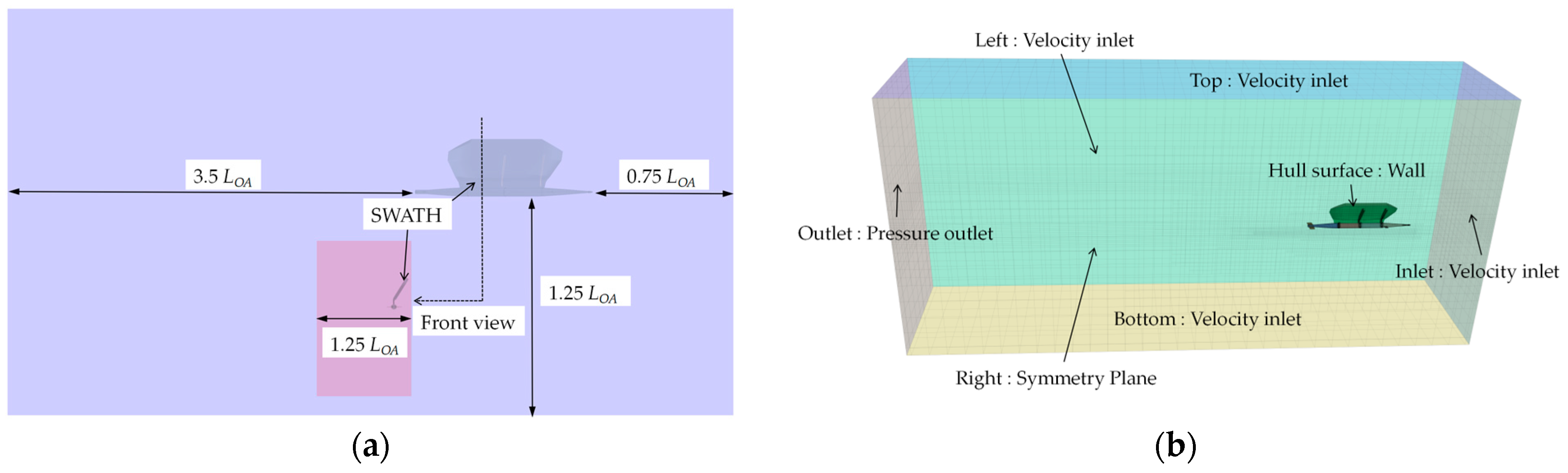
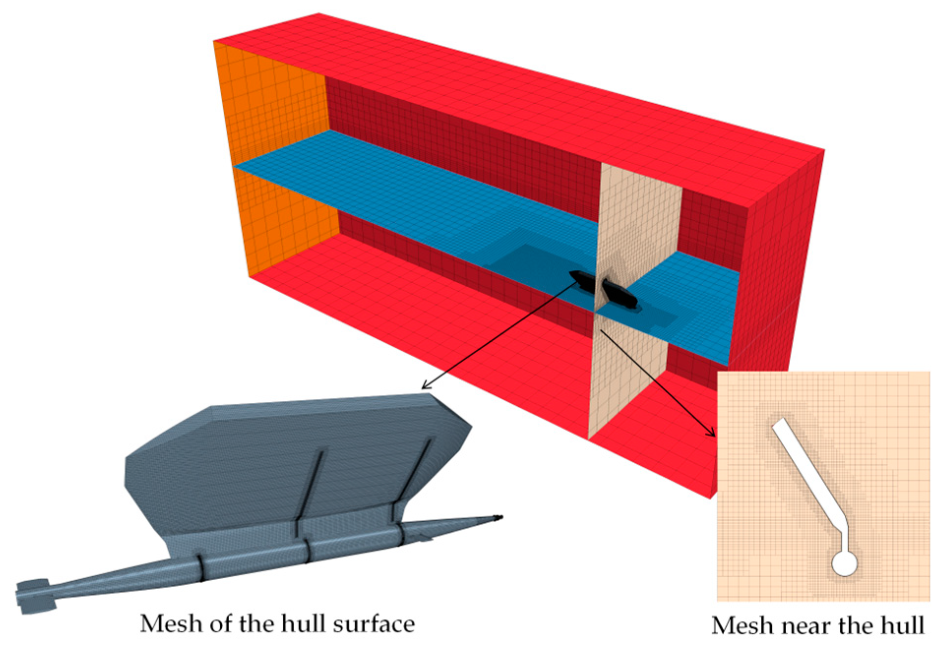
The computational domain size and boundary conditions are shown in Figure 1. The total length of the domain is 5.25, the total width is 1.25, and the water depth is 1.25. is the overall length of the SWATH. The position of the SWATH relative to the domain is shown in Figure 1a. The boundary condition of the domain can be seen in Figure 1b. The velocity inlet includes the Inlet, Left, Top, and Bottom. The Outlet is a pressure outlet, while the Right is a symmetry plane. The SWATH surface is a Wall, while the air gap is a Flow-Rate inlet. The mesh around the SWATH is refined, and the air gaps mesh adopts a finer mesh to ensure at least three layers of grids can be generated at the air gaps. In addition, the mesh at the free surface around the SWATH is refined for the Kelvin wake solution, where the longitudinal and transverse dimensions of the mesh are reduced, and the longitudinal and transverse dimensions are the same. The simulation mesh is shown in Figure 2.

Figure 1.
Detail of the domain: (a) Size; (b) Boundary conditions.

Figure 2.
Mesh of the computational domain.
3. Numerical Mesh Verification
3.1. SWATH Model
A SWATH model consisting of a slender underwater body and an inclined strut is used. Table 1 shows some parameters of the SWATH model.

Table 1.
Primary dimension characteristics.
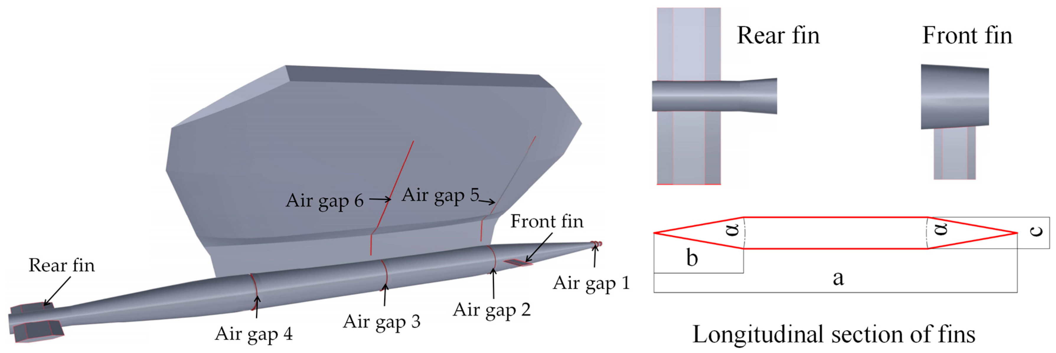
In this study, air gaps are used to inject the airflow. The air gaps are located in various places on the hull, as seen in Figure 3. There are four sets of air gaps on the underwater body, one set in the bow, and three in the middle. The longitudinal distances between the air gaps on the underwater body and stern are 2.5 m, 1.795 m, 1.265 m, and 0.748 m, respectively. Two sets of air gaps are located on the strut, with longitudinal distances between the air gaps on the strut and the stern of 1.765 m and 1.223 m.
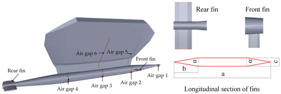
Figure 3.
The SWATH model and the details of the fins.
The locations and details of the fins are shown in Figure 3. The longitudinal distance between the center of the front fin and the stern is 0.067 m, and that from the rear fin to the stern is 1.767 m. The projected areas of the front and rear fins are 0.0063 m2 and 0.0303 m2. The primary characteristics of the fins’ longitudinal sections are shown in Figure 3, where, for the front fin, , , and , and, for the rear fin, , , and .
3.2. Verification and Validation
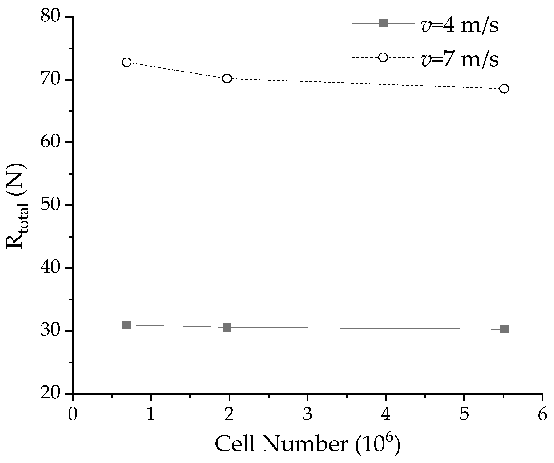
Grid convergence verification is an important test to judge whether a set of numerical meshes can be used for computation. The numerical meshes are verified before being used to calculate the resistance. The largest airflow rate used in this study, 6 L/s, is selected for the grid convergence test. The SWATH is advancing at a speed of and . The verification parameter is the total resistance . Three meshes with different cell sizes are built, which are named Fine, Medium, and Coarse. The mesh size of the Medium is decreased or increased by a factor to obtain the Fine or Coarse meshes [26], as shown in Table 2. The cell numbers of the Fine (), Medium (), and Coarse () meshes are , , and , respectively. The correlation parameter of the uncertainty analysis can be seen in Table 2, and the calculation process is as follows [26]:
where is the convergence ratio. , and is the resistance result of Mesh . is the accuracy order, and is the first-order Richardson extrapolation. is used in Equation (6). is the correction factor. is the uncertainty.
Table 2.
Results of mesh uncertainty test.
The results of total resistance are shown in Figure 4, corresponding to the different grids employed. The results of and are both monotonic with the number of cells. The difference between the results of the Medium and Fine meshes is acceptably small, and so the Medium () mesh could be considered appropriate.

Figure 4.
Grid convergence tests.
The calculation results and process of the mesh uncertainty are shown in Table 2, which are calculated by Equations (3)–(7). It can be seen that the of and are 0.609 and 0.506, respectively. There are significant differences between and 1, which means that the calculation process and results are reasonable, according to the ITTC recommendation [26]. is the uncertainty of a case. The of and are 3.86% and 1.77%, respectively, which means that the uncertainty is acceptable [26].
The experiment results for validation are provided in reference [25]. The numerical simulation grid is used to calculate the resistance under the experimental condition. In this study, a single hull is used for numerical simulation, and the calculated airflow rate is correspondingly half of the airflow rate of the experiment. The speed of the numerical simulation is 7 m/s. The resistance of a bare hull and a hull with fins is calculated, and the results can be seen in Table 3. is the resistance of the hull with fins by the CFD method. is the resistance of the bare hull by the CFD method. is the resistance of the bare hull by the experiment.
Table 3.
Results by CFD and experiment.
The resistance error of the numerical simulation and experiment is 2.21%. The resistance of the SWATH with fins is increased by 16.88% compared with that of the bare SWATH.
4. Results and Discussion
4.1. Effect of Trim Angle
The resistance and resistance reduction rate under different trim angles are studied by numerical simulation. is the trim angle of the SWATH. is positive when the SWATH is in the state of trim by the head. In different numerical simulation cases, the speed or the airflow rates are changed. is the airflow rate of a single injection gap, and the q of all injection gaps are the same in a case. Table 4 shows the information regarding the numerical simulation conditions for different cases.
Table 4.
Working conditions with different trim angles.
The total resistance and the total resistance reduction rate are shown in Figure 5. , where is the total resistance of L/s and is the total resistance of L/s or 6 L/s.
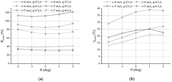
Figure 5.
The computing resistance and corresponding reduction rate under different trim angles: (a) Computing total resistance ; (b) Corresponding reduction rate .
It can be seen that the change in trim angle can affect the total resistance under different speeds and airflow rates, as shown in Figure 5a. The effect of the trim angle on the total resistance is more obvious in high-speed cases. In the cases without airflow, the minimum total resistance appears at the trim angle of −1 deg. In the high-speed cases with airflow, the minimum total resistance appears at the trim angle of 0 deg. As the airflow rate increases, the of trim by the head is gradually smaller than that of the trim by the stern. At the low speed with airflow, the total resistance at trim angles of 0 deg and 1 deg is close. As shown in Figure 5b, the reduction rate of total resistance with a positive trim angle is greater than that with a negative trim angle. This means the trim by the head is more conducive to total resistance reduction. For example, at the conditions of m/s and L/s, the total resistance reduction rate is 38.6% when the angle of trim by the head is 2 deg, while it is 29.04% when the angle of trim by the stern is −2 deg. The larger angle of trim by the head is more conducive to the total resistance reduction in the cases at low speed with airflow. The total resistance reduction rate is the largest at high speed when the angle of trim by the head is 1 deg. In summary, the slight trim by the head is more conducive to the total resistance reduction with airflow.
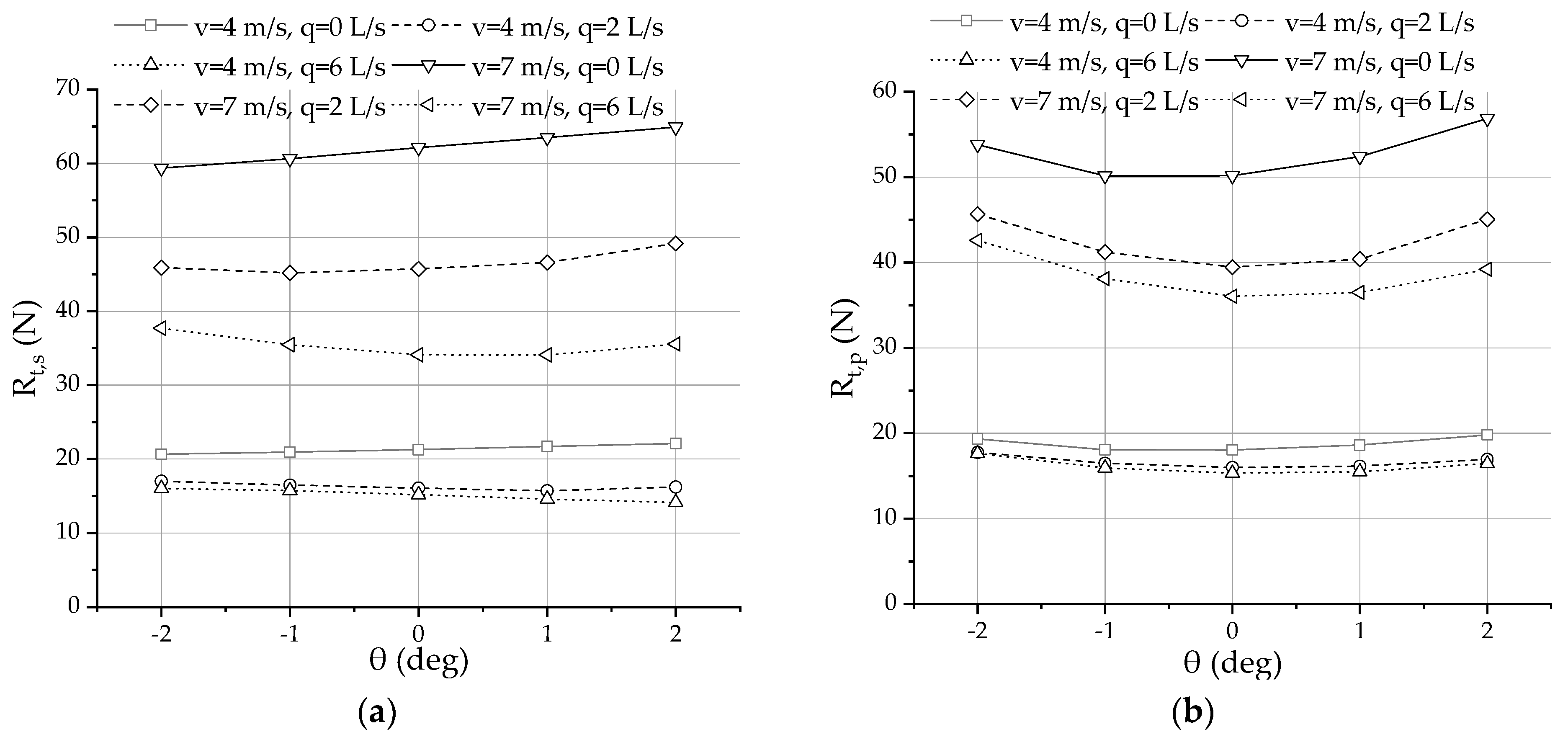
The resistance components in the cases of different trim angles are shown in Figure 6. Where is the resistance component about the shear, is the resistance component about the pressure.
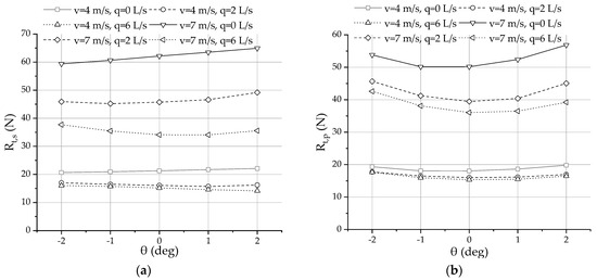
Figure 6.
Resistance component with different trim angles: (a) About the shear ; (b) About the pressure .
Figure 6a shows that at the conditions of L/s, the resistance component gradually increases with the trim angle getting larger, which means that the of the trim by the stern is smaller than that of the trim by the head. In the curve of m/s and L/s, when the trim angle is −2 deg, 0 deg, and 2 deg, the corresponding are 20.676 N, 21.291 N, and 22.118 N, respectively. In the curve of m/s and L/s, when the trim angle is −2 deg, 0 deg, and 2 deg, the corresponding are 59.354 N, 62.152 N, and 64.933 N, respectively. After the airflow was injected, decreases at different trim angles. In the cases of m/s and L/s, gradually decreases with the increase of , and the minimum is 15.733 N when the trim angle is 1 deg. After increasing the airflow rate to 6 L/s, the minimum is 14.15 N with the trim angle of 2 deg. In the cases of m/s and L/s, the minimum is 45.198 N with the trim angle of −1 deg. After increasing the airflow rate to 6 L/s, the minimum is 34.084 N with the trim angle of 1 deg. With the airflow rate increased, the resistance component with the trim by the head is gradually smaller than that with the trim by the stern. As shown in Figure 6b, the has the same trend under different speeds and airflow rates. With the increase of the trim angle , the resistance component decreases gradually, and it increases gradually after reaching the valley point. When the trim angle is 0 deg, the is the smallest. At the speed of 4 m/s, the smallest under the airflow rates of 0 L/s, 2 L/s, and 6 L/s are 18.04 N, 16.004 N, and 15.353 N, respectively. At the speed of 7 m/s, the smallest under the airflow rates of 0 L/s, 2 L/s, and 6 L/s are 50.171 N, 39.459 N, and 36.036 N, respectively. It could be seen that the of the upright hull attitude is the smallest. When the SWATH trim by the head or the stern appears, the pressure force increases.
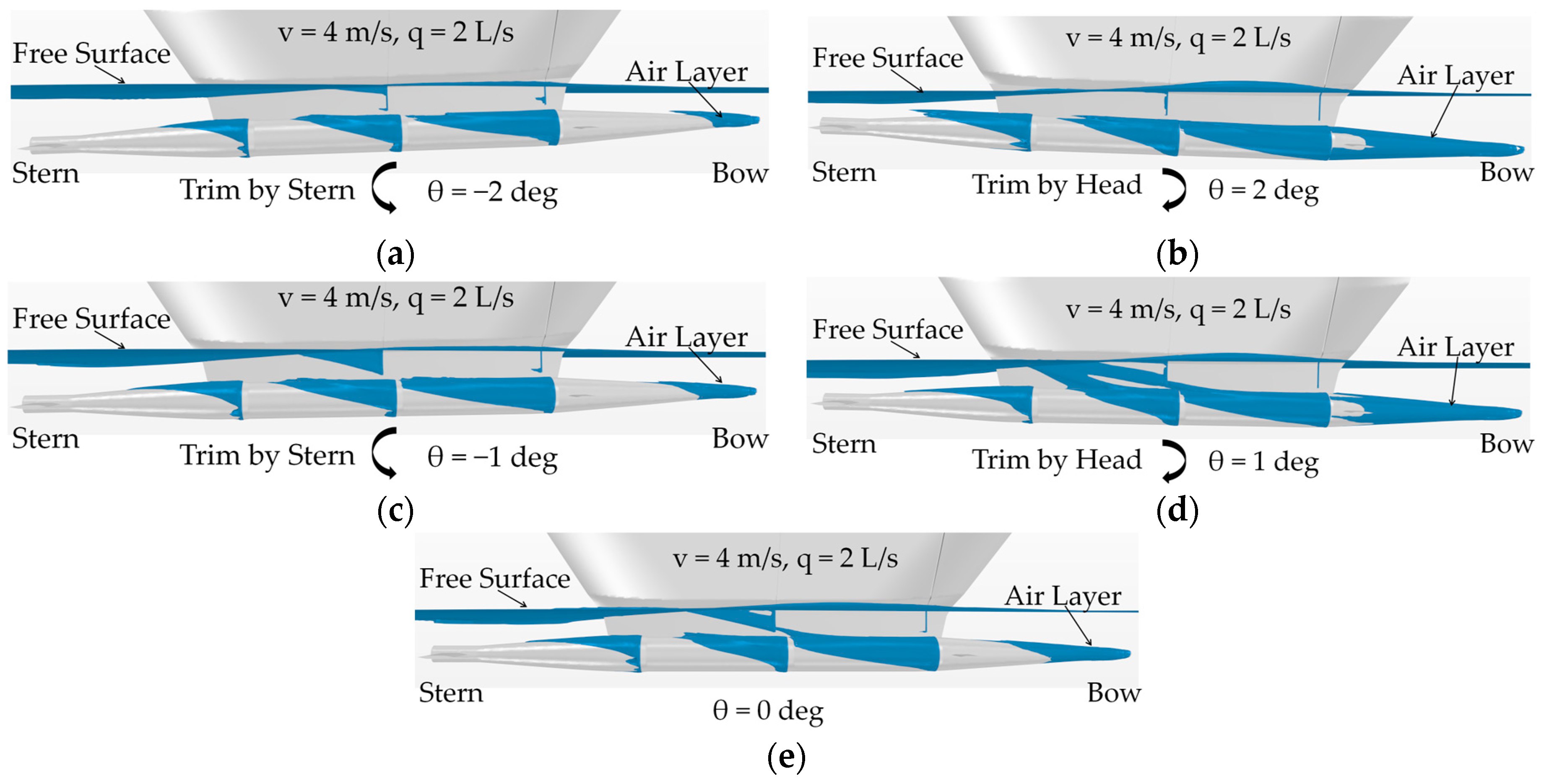
At different trim angles, the air layer coverage of the SWATH is different, which is shown in Figure 7, Figure 8, Figure 9 and Figure 10.
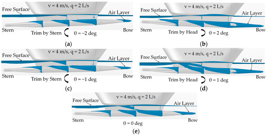
Figure 7.
Air coverage of m/s and L/s: (a) = −2 deg; (b) = 2 deg; (c) = −1 deg; (d) = 1 deg; (e) = 0 deg.
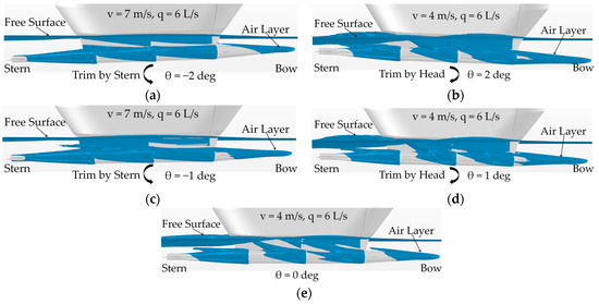
Figure 8.
Air coverage of m/s and L/s: (a) = −2 deg; (b) = 2 deg; (c) = −1 deg; (d) = 1 deg; (e) = 0 deg.
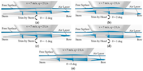
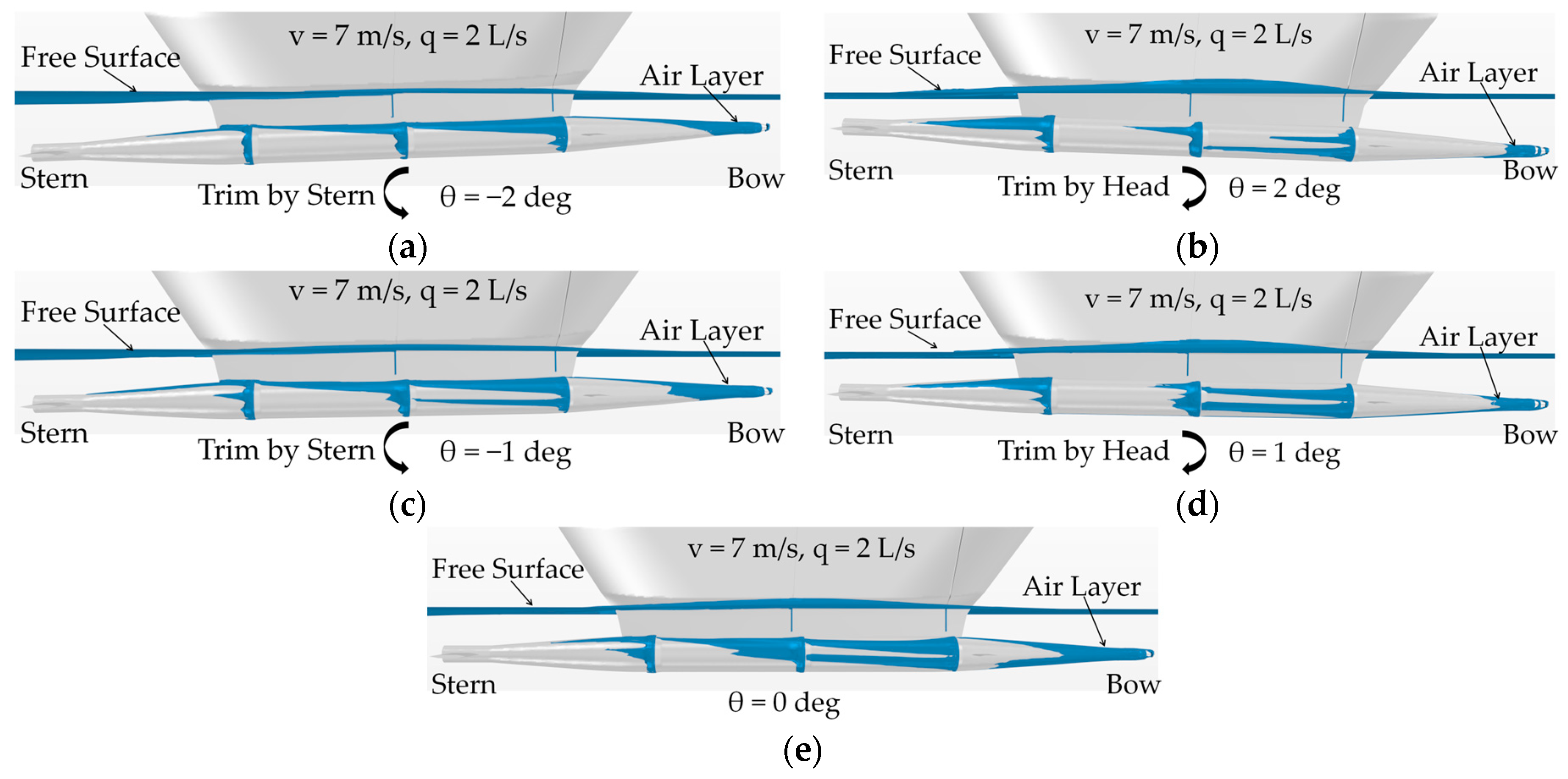
Figure 9.
Air coverage of m/s and L/s: (a) = −2 deg; (b) = 2 deg; (c) = −1 deg; (d) = 1 deg; (e) = 0 deg.
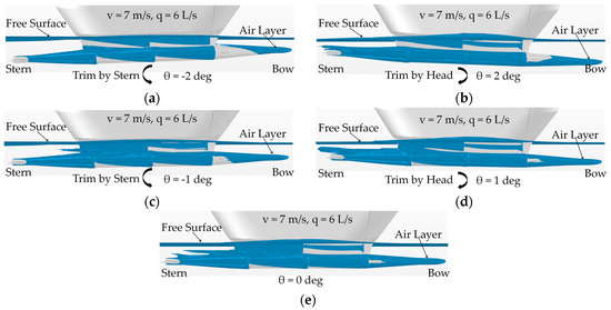
Figure 10.
Air coverage of m/s and L/s: (a) = −2 deg; (b) = 2 deg; (c) = −1 deg; (d) = 1 deg; (e) = 0 deg.
Figure 7 shows the air coverage of m/s and L/s with different trim angles. It could be that under the action of buoyancy, the airflow tends to float up, which makes the coverage of air in the upper part of the underwater body. With the increase in the trim angle, the sailing attitude gradually changes from the trim by the stern to the trim by the head, and changes of air coverage at the head of the underwater body are obvious. The air layer distribution with the trim angles of 1 deg and 2 deg is better than that of other trim angles, which results in greater total resistance reduction.
Figure 8 shows the air coverage of m/s and L/s with different trim angles. It could be that with the trim angle increasing, the air coverage trend is similar to that of the airflow rate 2 L/s. But, the air layer distribution at each trim angle is significantly greater than that of L/s.
Figure 9 shows the air coverage of m/s and L/s with different trim angles. When 0 deg, the air mainly covers the upper part of the underwater body. With the increase of , the air covering area increases gradually. The air coverage of 0 deg is the best. The trim angle continues to increase, and the SWATH changes to the trim by the head. When the trim angle is 2 deg, the air layer coverage area is smaller than that of 1 deg. This means that in the conditions of m/s and L/s, the trim by the head is not conducive to the air covering, and the larger the angle of the trim by the head, the worse the covering of the air.
Figure 10 shows the air coverage of m/s and L/s with different trim angles. It could be that the air coverage of −2 deg and −1 deg is better than that of 0 deg, 1 deg, and 2 deg. This means that in the conditions of m/s and L/s, the trim by the stern is not conducive to covering the air. At the trim angle of 2 deg, the air layer distribution of the strut and the underwater body bow is weaker than that at the trim angle of 2 deg. It could be inferred that as the angle of the trim by the head continues to increase, the air coverage of the SWATH will become worse.
A comprehensive analysis of Figure 7, Figure 8, Figure 9 and Figure 10 shows that no matter the speed and airflow rate, the trim by the stern is not conducive to the air coverage of the SWATH. At a low speed, the air coverage under the trim by the head is best. The air layer under the upright sailing attitude and the slight trim by the head could cover a larger area at a high speed.
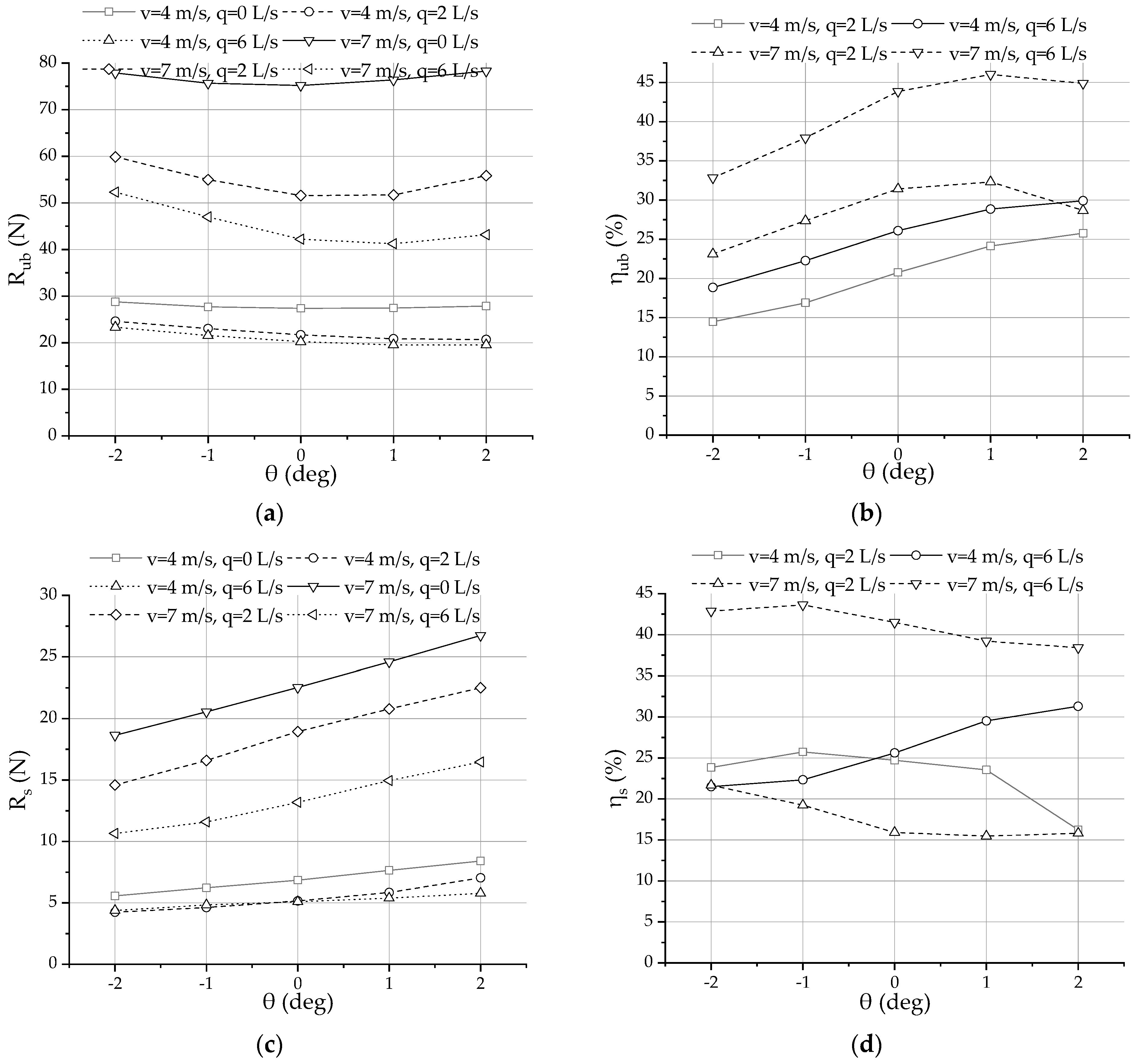
The computing resistance and corresponding reduction rate of different areas are shown in Figure 11. Where is the resistance of the underwater body, is the resistance of the strut, is the resistance reduction rate of the underwater body, and is the resistance reduction rate of the strut.

Figure 11.
The computing resistance and corresponding reduction rate of different areas under different trim angles: (a) Computing resistance of the underwater body ; (b) Corresponding reduction of the underwater body ; (c) Computing resistance of the strut ; (d) Corresponding reduction rate of the strut .
The change of the trim angle could affect the underwater body resistance under different speeds and airflow rates, and the influence of the trim angle is more obvious at a high speed, as shown in Figure 11a. In the working condition of m/s, the trim angle has a slight influence on the resistance of the underwater body without airflow. In the working condition of 7 m/s, the influence of the trim angle on the underwater body resistance is obvious, especially in the cases with airflow injection. In the working condition of m/s and 0 L/s, the smallest underwater body resistance is 75.17 N with 0 deg. When the airflow rate increases to 2 L/s, the underwater body resistances under the trim angles of 0 deg and 1 deg are smaller and close, which are 51.56 N and 51.69 N. When the airflow rate increases to 6 L/s, the smallest underwater body resistance is 41.22 N with 1 deg. It can be seen that a small trim angle by the head can lead to a small underwater body resistance with the airflow injection.
The trend of the resistance curve about the trim angles is the same under the same speed and different airflow rates, as shown in Figure 11b. The underwater body resistance reduction rate of the trim by the head is larger than that of the trim by the stern and upright attitude with m/s. For the curve of 2 L/s and 6 L/s, the maximum resistance reduction rates of the underwater body are 25.76% and 29.91%, respectively, with 2 deg. In the working condition of m/s, the underwater body resistance reduction rate with 1 deg is the largest. For the curve of 2 L/s and 6 L/s, the maximum resistance reduction rates of the underwater body are 32.31% and 46.02%, respectively, when the trim angle is 1 deg.
Figure 11c shows the resistance of the strut with different trim angles. It can be seen that with the increase of , the increases gradually. The strut resistance under the trim by the stern is smaller than that under the upright attitude and the trim by the head.
The of the trim angle of 2 deg is the largest with m/s and 2 L/s, while it is the smallest with m/s and 6 L/s, as shown in Figure 11d. This is because it is difficult for the airflow to cover the front part of the strut unless the airflow rate is large enough. In the working condition of 7 m/s, the strut resistance reduction rate of the trim by the head is larger than that of the trim by the stern and the upright attitude. For the curve of 2 L/s and 6 L/s, the maximum is 32.31% and 46.02%, respectively, when the trim angle is 1 deg.
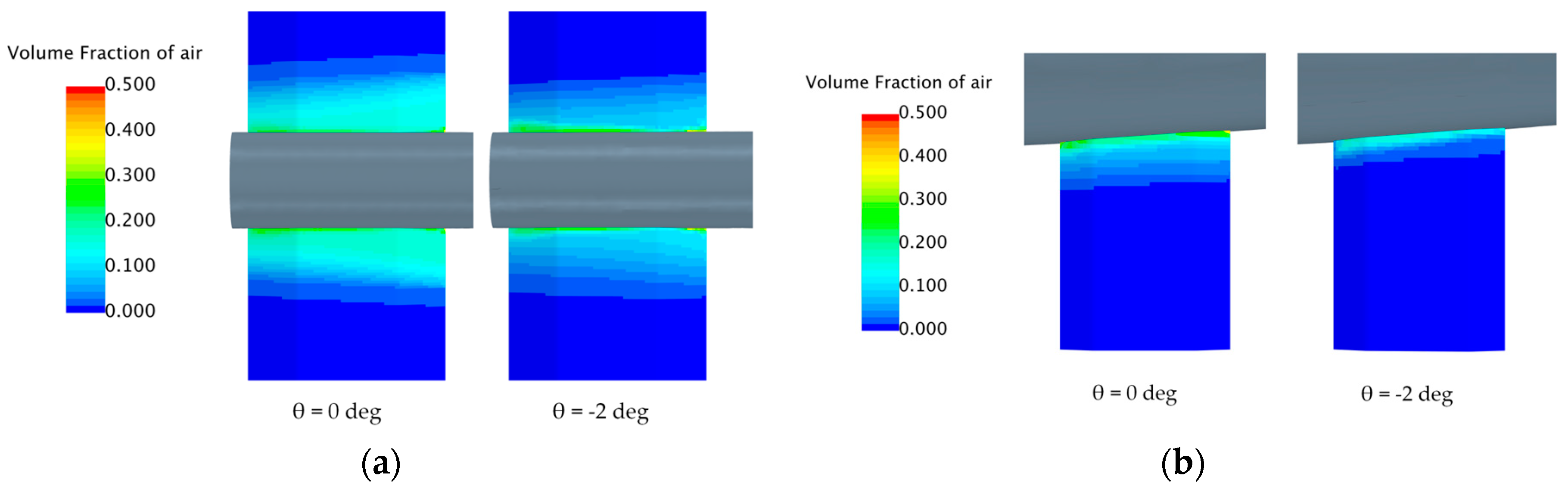
The airflow affects the air volume fraction of the fin surface, especially where the fins join the hull, and the air volume fraction of the fins is different at different trim angles. For example, Figure 12 shows the air volume fraction of the fins with 0 deg and −2 deg in the working conditions of 7 m/s and 6 L/s.

Figure 12.
Air volume fraction of the fins, 7 m/s and 6 L/s: (a) Rear fin; (b) Front fin.
It can be seen that the air volume fraction at the connection between the fins and the hull is between 0.1 and 0.3. When the trim angle is 0 deg, the area affected by the airflow on the front and rear fins is greater than that when the trim angle is −2 deg. The influence of the trim angle on the resistance reduction of the fins is studied, too. The resistance reduction rate of the front fin and the rear fin is shown in Figure 13, where is the resistance reduction rate of the front fin and is the resistance reduction rate of the rear fin.
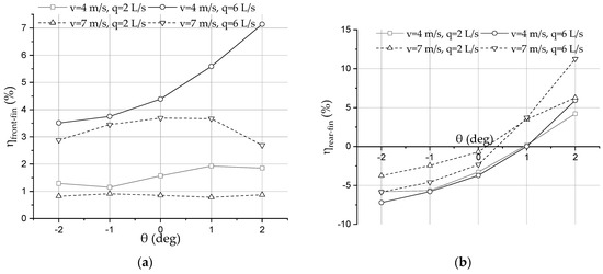
Figure 13.
Resistance reduction rate of the fore fin and the aft fin with different trim angles: (a) Resistance reduction rate of the fore fin; (b) Resistance reduction rate of the aft fin.
It can be seen that the resistance reduction rate of the front fin is greater than 0 in all numerical cases, as shown in Figure 13a. The resistance reduction effect is different under different speeds and airflow rates. The of 4 m/s and 6 L/s is greater than that at other speeds and airflow rates. The is minimal with 7 m/s and 2 L/s. The increase in speed is not conducive to the resistance reduction of the front fin, while the increase in the airflow rate is conducive to the resistance reduction of the front fin. In the working condition of 4 m/s, the increases gradually with the increase of the trim angle. This means that the trim by the head is advantageous for the resistance reduction of the front fin. In the working conditions of 7 m/s and 6 L/s, the with the trim angle of 2 deg is the smallest. The resistance reduction effect of the front fin could be reduced if the trim angle by the head is too large at a high speed and high airflow rate.
It can be seen that when the trim angle is 0 deg, the resistance reduction rate of the rear fin is less than 0, as shown in Figure 13b. When the SWATH is under the trim by the head and the upright attitude, the airflow could increase the resistance of the rear fin. When the trim angle is >0 deg, the is >0 and the of 6 L/s is larger than that of 2 L/s. The trim by the head is beneficial for the resistance reduction of the aft fin, and the resistance reduction of the rear fin could be improved by increasing the airflow rate under the trim by the head.
4.2. Effect of the Draft
This section studies the resistance and resistance reduction rates under different drafts. The numerical simulation conditions for different cases are shown in Table 5.
Table 5.
Working conditions with different drafts.
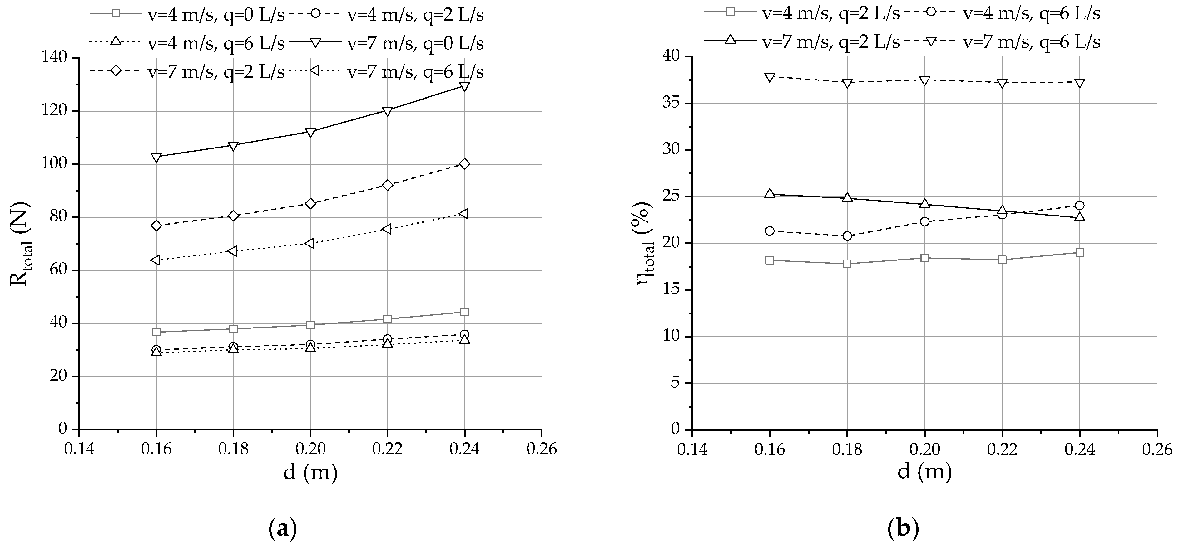
The total resistance and total resistance reduction rate are shown in Figure 14.

Figure 14.
The computing resistance and corresponding reduction rate under different drafts: (a) Computing total resistance ; (b) Corresponding reduction rate .
It can be seen that the difference between the total resistance of 2 L/s and that of 6 L/s under different drafts with 4 m/s is smaller than the difference of 7 m/s, as shown in Figure 14a. Regardless of the draft, the smaller airflow rate at a low speed could significantly reduce the resistance, and the larger airflow rate at a high speed could lead to a smaller total resistance. As shown in Figure 14b, the gradually increases with the increase of the draft at 4 m/s, while that gradually decreases with the increase of the draft at 7 m/s. In the working condition of 4 m/s, the largest of 2 L/s and 6 L/s is 19.01% and 24.05% with the draft of 0.24 m. When the speed is 6 m/s, the largest of the airflow rate of 2 L/s and 6 L/s is 19.01% and 24.05% with the draft of 0.16 m. With the increase in the draft, increasing the airflow rates at a high speed is more conducive to improving the total resistance reduction.
The resistance components in the cases of different drafts are also studied, where is the resistance component about the shear and is the resistance component about the pressure. Both and increase with the draft, which is similar to the total resistance. But, the sensitivity of and to the draft are different, as shown in Table 6. , , , and are given as follows:
where and are the resistance components about the shear at the draft of 0.16 m and 0.24 m, and and are the resistance components about the pressure at the draft of 0.16 m and 0.24 m.
Table 6.
Effect of the draft on the resistance components.
As shown in Table 6, both and are positive at any speed and airflow rate. Both and increase with the draft. is between 33.30% and 48.86%, while is between 7.51% and 14.52%. It can also be seen that is much bigger than , as shown in Table 5. The draft has a greater influence on than . The increase in the draft increases the proportion of the in the total resistance.
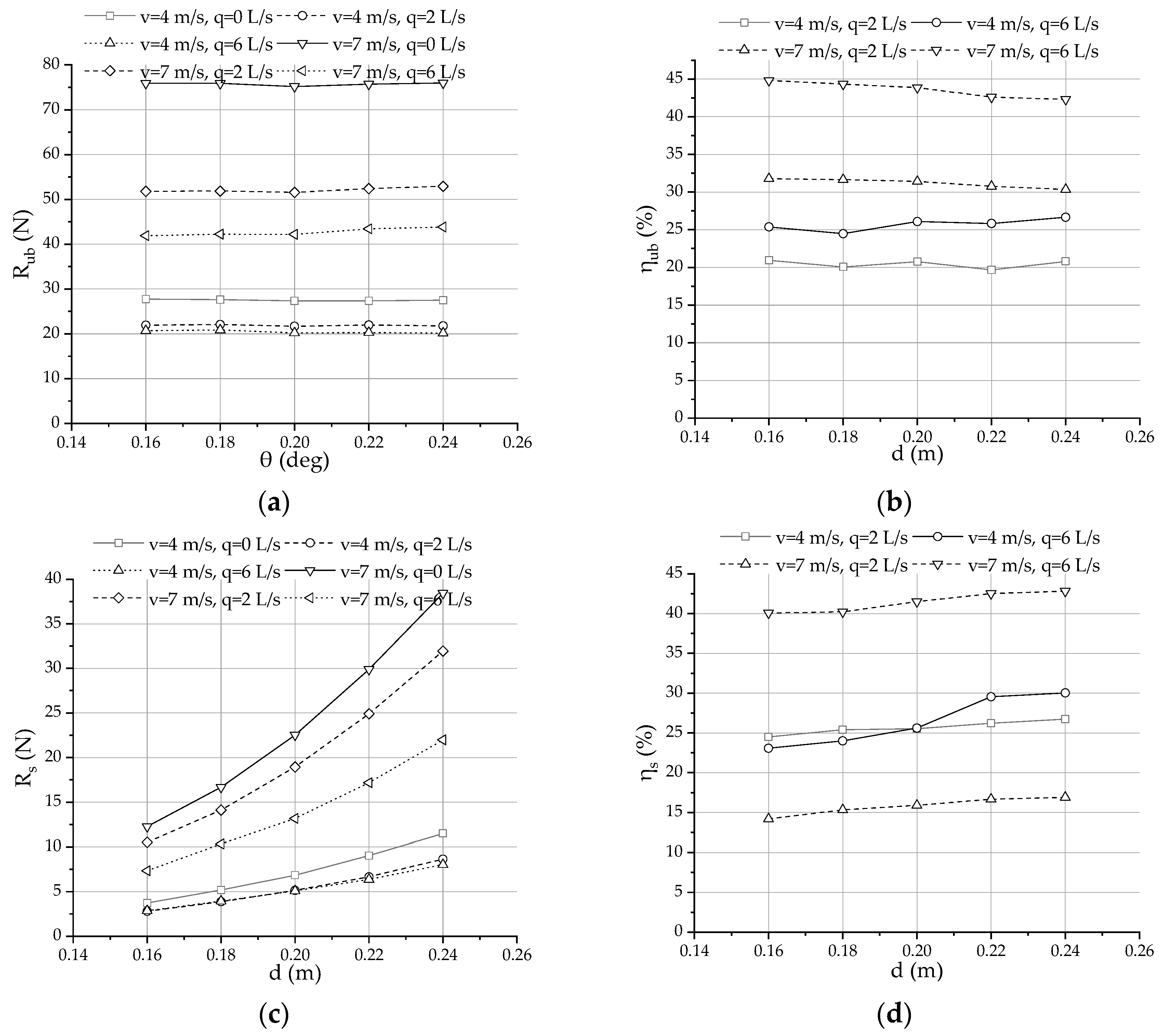
The computing resistance and corresponding reduction rate of different areas are shown in Figure 15.

Figure 15.
The computing resistance and corresponding reduction rate of different areas under different drafts: (a) Computing resistance of the underwater body ; (b) Corresponding reduction of the underwater body ; (c) Computing resistance of the strut ; (d) Corresponding reduction rate of the strut .
is less affected by the draft with 0 L/s, as shown in Figure 15a. However, the effect of the draft on can still be observed at the airflow rate of 2 L/s and 6 L/s, especially at a high speed of 7 m/s. For example, when the speed is 7 m/s, an increase in the draft from 0.16 m to 0.24 m will increase the resistance of the underwater body by 1.94 N. This results in the phenomenon that decreases with the increase of the draft at 7 m/s, as shown in Figure 15b. The surface pressure of the underwater body gets larger by the increasing draft, which makes the air coverage worse and reduces . As shown in Figure 15c, it can be seen that with the increase of the draft, increases obviously. The increase in the draft causes the wet surface area of the strut to increase. It can be seen that increases gradually by the increasing draft, as shown in Figure 15d. This is because the increased wet surface area provides a larger potential coverage area for the air layer.
5. Conclusions
In this paper, the resistance of a SWATH at different trim angles and drafts is calculated by numerical methods. There are differences in the speed or the airflow rate in different cases. The relationship between the hull attitude and the resistance reduction is investigated, and the air coverage on the surface under different hull attitudes is observed. This study shows the effect of the hull attitudes on the air coverage and drag reduction of the SWATH. The numerical model used in this paper is suitable for drag reduction calculation under air layer cover, but it is weak in the monitoring of micro-bubbles and air leaving the surface. However, the current numerical method is validated, and the accuracy of the resistance calculation meets the requirements. The conclusions are as follows.
Firstly, the influence of trim angles on the total resistance reduction after airflow is injected is more evident at a high speed. The slight trim by the head leads to a more significant total resistance reduction of the SWATH. The total resistance reduction of the cases with the trim angle of 1 deg can reach 39.11%, which is greater than that of other trim angles. At a low speed, the total resistance reduction rate gradually increases with the increase of the draft, while it gradually decreases at high speeds. Increasing the draft requires increasing the airflow rate to achieve sufficient resistance reduction at high speeds. When the draft increases from 0.16 m to 0.24 m, the resistance component about the shear increases by more than 33%, while the resistance component about the pressure increases by less than 15%. The increase in the draft increases the proportion of the component about the shear.
Secondly, resistance reduction in different areas is studied. The trim by the stern can lead to a smaller resistance and a larger resistance reduction rate of the strut at a high speed. At a low speed, the resistance reduction of the trim by the head is better than that of the trim by the stern when increasing the airflow rate. At high drafts, the resistance reduction of the strut is greater than that at low drafts. The maximum resistance reduction of the high draft is 42.81%, while that of the low draft is 10%.
Thirdly, the resistance reduction of the front and rear fins at different trim angles is analyzed. The resistance reduction of the front fin could be reduced if the angle of the trim by the head is too large at high speeds and airflow rates. When the speed is 7 m/s, and the airflow rate is 6 L/s, the resistance reduction of the front fin with the trim angle of 2 deg is 2.69%, which is smaller than that of 1 deg with a value of 3.67%. The trim by the head is beneficial for the resistance reduction of the rear fin. With the attitude of the trim by the head, the resistance reduction of the rear fin can reach 11.26%. The resistance reduction of the aft fin could be improved by increasing the airflow rate under the trim by the head. The airflow injection could increase the resistance of the rear fin under the trim by the stern and the upright attitude, and, at different airflow rates and speeds, the rate of the resistance increase varies, ranging from 0.69% to 7.2%.
Author Contributions
Conceptualization, D.Z. and Y.L.; methodology, D.Z. and Z.F.; software, D.Z.; validation, D.Z. and J.G.; formal analysis, D.Z.; investigation, D.Z. and J.G.; resources, Y.L.; data curation, D.Z.; writing—original draft preparation, D.Z. and Z.F.; visualization, D.Z.; supervision, D.Z. and Y.L.; project administration, D.Z.; funding acquisition, Y.L. All authors have read and agreed to the published version of the manuscript.
Funding
This project was supported by the National Natural Science Foundation of China, grant number 51979157, and the Science and Technology Commission of Shanghai Municipality, China, grant number 22YF1415900.
Institutional Review Board Statement
Not applicable.
Informed Consent Statement
Not applicable.
Data Availability Statement
No new data are created or analyzed in this study. Data sharing is not applicable to this article.
Conflicts of Interest
The authors declare no conflict of interest.
References
- Winebrake, J.; Corbett, J.; Meyer, P. Energy use and emissions from marine vessels: A total fuel life cycle approach. J. Air Waste Manag. Assoc. 2007, 57, 102–110. [Google Scholar] [CrossRef] [PubMed]
- Cucinotta, F.; Guglielmino, E.; Sfravara, F. Life cycle assessment in yacht industry: A case study of comparison between hand lay-up and vacuum infusion. J. Clean. Prod. 2017, 142, 3822–3833. [Google Scholar] [CrossRef]
- Uyanık, T.; Karatuğ, Ç.; Arslanoğlu, Y. Machine learning approach to ship fuel consumption: A case of container vessel. Transp. Res. Part. D 2020, 84, 102389. [Google Scholar] [CrossRef]
- Karatuğ, Ç.; Arslanoğlu, Y.; Soares, C.G. Evaluation of decarbonization strategies for existing ships. In Trends in Maritime Technology and Engineering; CRC Press: Boca Raton, FL, USA, 2022; ISBN 9781003320289. [Google Scholar]
- Vernengo, G.; Brizzolara, S. Numerical investigation on the hydrodynamic performance of fast SWATHs with optimum canted struts arrangements. Appl. Ocean Res. 2017, 63, 76–89. [Google Scholar] [CrossRef]
- Qian, P.; Yi, H.; Li, Y. Numerical and experimental studies on hydrodynamic performance of a small-waterplane-area-twin- hull (swath) vehicle with inclined struts. Ocean Eng. 2015, 96, 181–191. [Google Scholar] [CrossRef]
- Butterworth, J.; Atlar, M.; Shi, W. Experimental analysis of an air cavity concept applied on a ship hull to improve the hull resistance. Ocean Eng. 2015, 110, 2–10. [Google Scholar] [CrossRef]
- Elbing, B.R.; Winkel, E.S.; Lay, K.A.; Ceccio, S.L.; Dowling, D.R.; Perlin, M. Bubble-Induced Skin-Friction drag reduction and the abrupt transition to Air-Layer drag reduction. J. Fluid Mech. 2008, 612, 201–236. [Google Scholar] [CrossRef]
- Elbing, B.R.; Mäkiharju, S.; Wiggins, A.; Perlin, M.; Dowling, D.R.; Ceccio, S.L. On the scaling of air layer drag reduction. J. Fluid. Mech. 2013, 717, 484–513. [Google Scholar] [CrossRef]
- Makiharju, S.; Ceccio, S. On multi-point gas injection to form an air layer for frictional drag reduction. Ocean Eng. 2018, 147, 206–214. [Google Scholar] [CrossRef]
- Latorre, R. Ship hull drag reduction using bottom air injection. Ocean Eng. 1997, 24, 161–175. [Google Scholar] [CrossRef]
- Murai, Y.; Fukuda, H.; Oishi, Y.; Kodama, Y.; Yamamoto, F. Skin friction reduction by large air bubbles in a horizontal channel flow. Int. J. Multiph. Flow 2007, 33, 147–163. [Google Scholar] [CrossRef]
- Murai, Y. Frictional drag reduction by bubble injection. Exp. Fluid. 2014, 55, 1773. [Google Scholar] [CrossRef]
- Slyozkin, A.; Atlar, M.; Sampson, R.; Seo, K.C. An experimental investigation into the hydrodynamic drag reduction of a flat plate using air-fed cavities. Ocean Eng. 2014, 76, 105–120. [Google Scholar] [CrossRef]
- Amromi, E.L. Analysis of interaction between ship bottom air cavity and boundary layer. Appl. Ocean Res. 2016, 59, 451–458. [Google Scholar] [CrossRef]
- Matveev, K.I. Hydrodynamic modeling of semi-planing hulls with air cavities. Int. J. Nav. Archit. Ocean Eng. 2015, 7, 500–508. [Google Scholar] [CrossRef]
- Cucinotta, F.; Guglielmino, E.; Sfravara, F. An experimental comparison between different artificial air cavity designs for a planing hull. Ocean Eng. 2017, 140, 233–243. [Google Scholar] [CrossRef]
- Cucinotta, F.; Guglielmino, E.; Sfravara, F.; Strasser, C. Numerical and experimental investigation of a planing Air Cavity Ship and its air layer evolution. Ocean Eng. 2018, 152, 130–144. [Google Scholar] [CrossRef]
- Jang, J.; Choi, S.H.; Ahn, S.-M.; Kim, B.; Seo, J.S. Experimental investigation of frictional resistance reduction with air layer on the hull bottom of a ship. Int. J. Nav. Arch. Ocean Eng. 2014, 6, 363–379. [Google Scholar] [CrossRef]
- Makiharju, S.; Perlin, M.; Ceccio, S. On the energy economics of air lubrication drag reduction. Int. J. Nav. Archit. Ocean. Eng. 2012, 4, 412–422. [Google Scholar] [CrossRef]
- Wu, H.; Ou, Y. Experimental study of air layer drag reduction with bottom cavity for a bulk carrier ship model. China Ocean Eng. 2019, 5, 554–562. [Google Scholar] [CrossRef]
- Wu, H.; Ou, Y. Analysis of air layer shape formed by air injection at the bottom of flat plate. Ocean Eng. 2020, 216, 108091. [Google Scholar] [CrossRef]
- Wu, H. Numerical study of the effect of ship attitude on the perform of ship with air injection in bottom cavity. Ocean Eng. 2019, 186, 106119. [Google Scholar]
- Song, L.; Yu, J.; Yu, Y.; Wang, Z.; Wu, S.; Gao, R. An experimental study on the resistance of a High-Speed air cavity craft. J. Mar. Sci. Eng. 2023, 11, 1256. [Google Scholar] [CrossRef]
- Zhang, D.; Li, Y.; Gong, J. Study on the effect of air injection location on the drag reduction of SWATH with air lubrication. J. Mar. Sci. Eng. 2023, 11, 667. [Google Scholar] [CrossRef]
- ITTC Recommended Procedures and Guidelines. Uncertainty analysis in CFD verification and validation-methodology and validation 7.5-03-01-01. In Proceedings of 28th International Towing Tank Conference, Wuxi, China, 18 September 2017. [Google Scholar]


Disclaimer/Publisher’s Note: The statements, opinions and data contained in all publications are solely those of the individual author(s) and contributor(s) and not of MDPI and/or the editor(s). MDPI and/or the editor(s) disclaim responsibility for any injury to people or property resulting from any ideas, methods, instructions or products referred to in the content. |
© 2023 by the authors. Licensee MDPI, Basel, Switzerland. This article is an open access article distributed under the terms and conditions of the Creative Commons Attribution (CC BY) license (https://creativecommons.org/licenses/by/4.0/).