Abstract
Studying the mechanical characteristics of hydrate-bearing sediments (HBS) contributes to the comprehensive understanding of the mechanical behavior in environments with natural gas hydrate (NGH) occurrences. Simultaneously, the distribution patterns of hydrates significantly influence the strength, deformation, and stability of HBS. Therefore, this paper employs particle flow code (PFC) to conduct biaxial discrete element simulations on specimens of HBS with different hydrate distribution patterns, revealing the macroscale–mesoscale mechanical properties, evolution patterns, and destructive mechanisms. The results indicate that the strain-softening behavior of HBS specimens strengthens with the increase in hydrate layer thickness, leading to higher peak strength and E50 values. During the gradual movement of the hydrate layer position (Ay) from both ends to the center of the specimen (Ay = 0.40 mm → Ay = 20 mm), the strain-softening behavior weakens. However, when Ay = 20 mm, the specimen exhibits evident strain-softening behavior again. Moreover, with an increase in the angle between the hydrate layer and the horizontal direction (α) greater than 20°, the peak strength of the specimen increases, while E50 shows an overall decreasing trend. The influence of axial loads on the hydrate layer in specimens varies with α, with larger contact forces and fewer cracks observed for higher α values.
1. Introduction
Natural gas hydrate (NGH), a crystalline cage-shaped solid complex formed via the interaction of water molecules and methane in situations of higher pressure and lower temperature, emerges as a promising clean alternative energy source when compared to traditional fossil fuels. Its distinct advantages, including high energy density, substantial reserves, and environmentally friendly characteristics, position NGH as a noteworthy prospect for the future [1,2,3,4]. However, the production of NGH poses significant risks to geological formations. The dissociation of NGH during production has the potential to initiate large-scale seafloor destabilization, resulting in adverse effects on geological structures [5,6,7]. Furthermore, the uncontrolled release of methane gas from NGH into the atmosphere has the potential to exacerbate the greenhouse effect, intensifying environmental concerns [8,9,10]. Consequently, to ensure the secure and efficient exploitation of NGH and to promote their commercialization, a critical necessity arises for the comprehensive study of their mechanical properties. This scholarly endeavor is indispensable for advancing our understanding and developing strategies for the responsible utilization of NGH across various sectors.
In the pursuit of expediting the commercial exploitation of NGH, scientists have carried out an abundance of experiments examining the mechanical characteristics of these NGH both in field settings and controlled laboratory environments, employing diverse testing methodologies. Wu Qi et al. [11] undertook triaxial shear experiments on HBS, revealing a close interconnection between shear and deformation properties and hydrate saturation, as well as net surrounding pressure. Hyodo et al. [12] meticulously executed a series of indoor triaxial shear tests on synthetic HBS, exploring the intricate effects of hydrate saturation, temperature, and net confining pressure on the strength and deformation attributes. Li et al. [13] in a complementary effort, conducted a series of indoor triaxial shear experiments to scrutinize the mechanical properties of HBS under horizontal layering conditions. Winters et al. [14], in turn, subjected HBS drilled from the Mackenzie Delta to rigorous testing, focusing on acoustic and shear properties. Yoneda et al. [15] extended the discourse by conducting triaxial compression tests on sandy and clayey pulverized HBS, employing pressure coring in the eastern part of the Nankai Trough, Japan. Luo et al. [16] contributed to this volume of work by contrasting the mechanical characteristics of in situ cores of HBS in the South China Sea with laboratory-prepared specimens, employing triaxial shear tests. Their findings indicated remarkable similarities in stress–strain characteristics and strength properties, confirming the capability of hydrate particles to enhance bonding between sediment particles. These studies collectively play a pivotal role in advancing our understanding of the intricate mechanical properties inherent in HBS. However, the current stage of development in relevant testing equipment and technology, compounded by the challenging storage conditions of hydrates in reservoirs, impedes the execution of a multitude of tests.
In order to overcome the limitations of existing indoor experimental techniques, scholars have carried out a series of numerical simulation studies in different dimensions. Zhu et al. [17] used the Tough + Hydrate to construct a 3D model of a hydrate reservoir, which proved the important impact of reservoir fluctuations and physical properties on gas hydrate recovery and emphasized the need to use more realistic 3D models for production dynamics prediction. Bosikov et al. [18] established a preliminary 4D geological model via 4D simulation and analyzed the characteristics of the geological model to evaluate multi-stage hydraulic fracturing parameters. And to study the mechanical properties of hydrate sediments, many scholars use the PFC to conduct numerical simulation studies. Jiang et al. [19,20,21,22] pioneered the establishment of a mesoscopic bonding model elucidating the mechanical characteristics of NGH. This model aims to reflect the intricate contact mechanical responses occurring between sediment particles under the influence of bonding. Subsequently, a comprehensive suite of discrete element simulation experiments complemented this foundational work. Wang et al. [23] introduced a PFC-based methodology to simulate the generation of pore-filling hydrates, meticulously exploring the mechanical properties under diverse conditions of confining pressure and saturation. Yu et al. [24], utilizing PFC, delved into the impact on the mechanical performance in triaxial compression experiments of soil shape and hydrate growth mode. Zhao et al. [25], leveraging PFC, conducted a meticulous analysis examining the impact of hydrate horizontal layering dispersion on the initial stress and failure stress of HBS. Their work yielded valuable insights into the damage law governing sediments containing NGH. Jiang et al. [26] employed PFC to investigate the effects of hydrate content and loading rate on various parameters, such as strength, stiffness, cohesion, and internal friction angle, within HBS. Their discrete element simulation [27] further explored shear strength, volumetric strain, and the evolutionary patterns of shear bands under different dynamic loading conditions. While these examinations have furnished an initial comprehension of the macroscopic and mesoscopic shear properties of HBS under triaxial shear conditions, it is imperative to acknowledge that different distributions of hydrates within HBS can significantly alter their mechanical properties [28,29,30]. A more in-depth comprehension of how the distribution patterns of hydrates influence the mechanical characteristics of HBS holds considerable promise in advancing the realization of long-term stable commercial production of NGH.
In consideration of the insights, to delve deeper into the impact of hydrate distribution patterns on the mechanical properties of HBS, this study employed the PFC for biaxial discrete element numerical simulations of specimens with varied arrangements of hydrate distribution patterns. The research focused on investigating the macroscale–mesoscale shear mechanical properties of the specimens, unveiling the destructive mechanisms. These research findings hold significant guidance for a more accurate understanding of the mechanical properties of HBS and provide insights for the management and mitigation of seabed geological hazards.
2. Discrete Element Method for PFC
2.1. Particle Contact Model
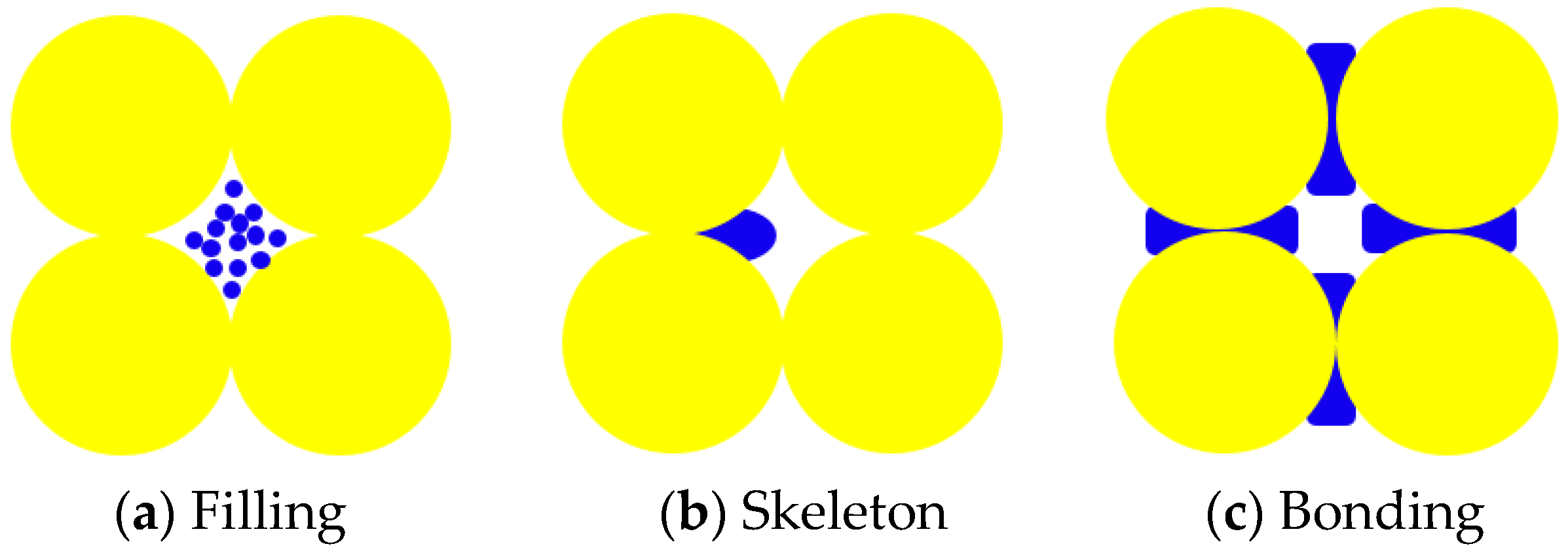
The mechanical characteristics of HBS are subject to various influencing factors. Beyond the well-established factors such as hydrate saturation and stress conditions, it can be significantly altered by the pattern of hydrate accumulation. Figure 1 illustrates the mesoscale distribution patterns of hydrates in three prevalent sediment structures: the filling pattern, the skeleton pattern, and the bonding pattern [31,32]. For this study, the hydrate accumulation pattern is of paramount importance. The hydrate most extensively distributed in nature is carefully selected as the basis for constructing the HBS model [33]. This choice is made to ensure the representation of the most common and prevalent hydrate distribution in natural settings. Consequently, the model adopted in this paper employs the hydrate distribution pattern that is most observed in nature, providing a realistic foundation for the investigation of the mechanical characteristics of HBS.
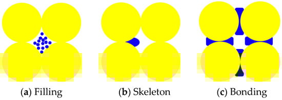
Figure 1.
Bonding types of HBS.
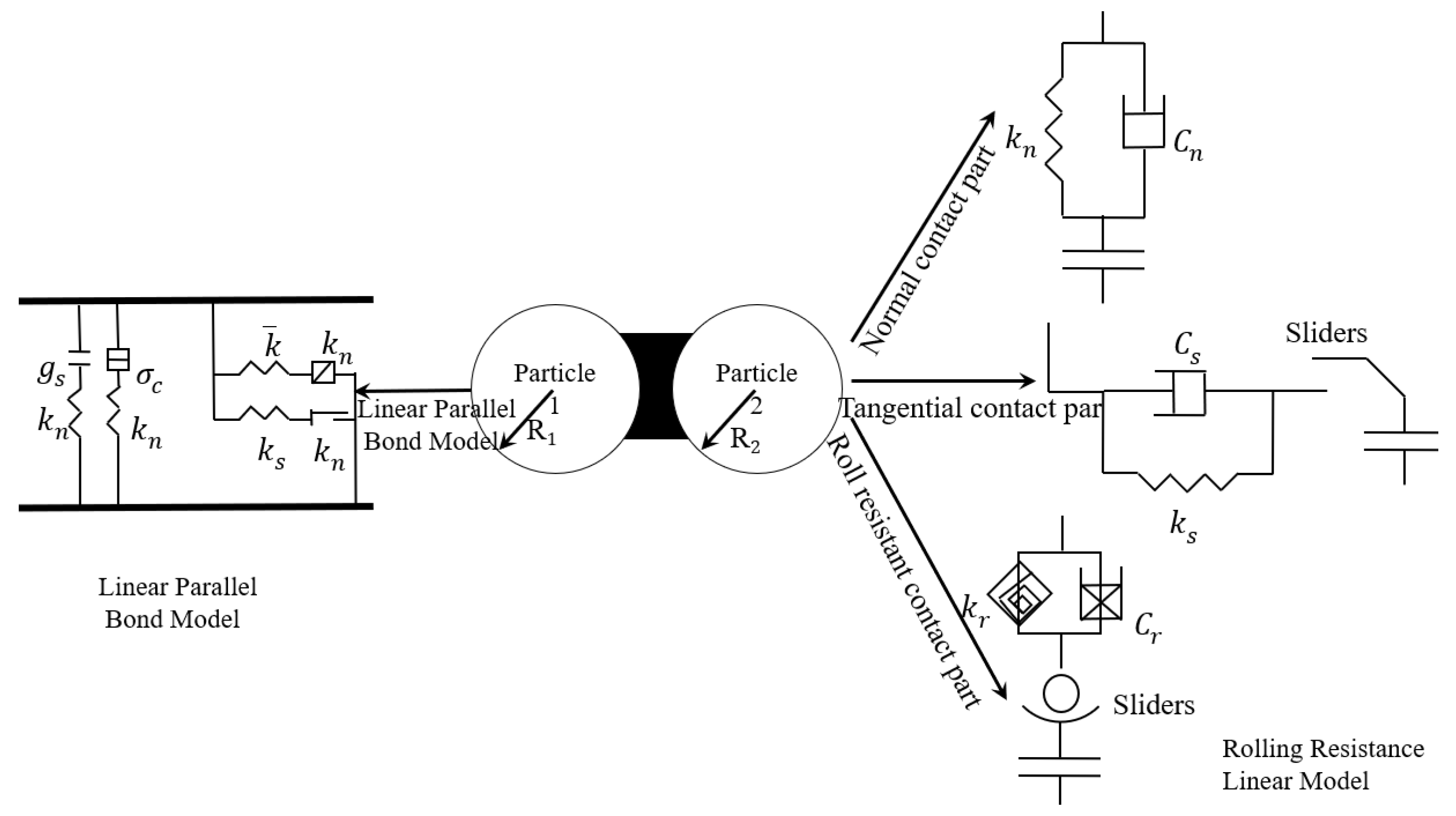
Taking into account the shape impact of sandy soil and the bonding influence between hydrate particles and soil particles, a linear contact model for rolling resistance and a bonding contact model in parallel were employed between sediment particles and between hydrate and soil particles, respectively [34]. As depicted in Figure 2, The linear contact model for rolling resistance incorporates the impact of rolling resistance on the foundation of the linear contact model, including the normal contact part, tangential contact segment, and anti-rolling contact segment. The complete rolling resistance linear contact model involves the normal contact force Fn, tangential contact force Fs, and anti-rolling moment MT, and its calculation formula is expressed as follows [35]:
where is relative angle increment and is rolling resistance stiffness.

Figure 2.
Conceptual map of particle contact model for HBS.
The relationship between contact force and displacement for the parallel bonding model is illustrated in Figure 2. It is evident that the contact force and displacement in the parallel bonding model depend on the contact stiffness and relative displacement between particles. Here, and denote the constituents of the contact force in the normal and tangential directions, respectively. represents the torque, represents the contact bending moment, represents the tangential displacement of the contact, is the rotation angle of the contact, and represents the torsion angle of the contact. The utmost normal contact force and maximum shear contact force on the contact surface can be computed based on the contact force and contact moment. Contact moment is as follows [35]:
where I, A, and J represent the cross-sectional moment of inertia, the cross-sectional area, and the cross-sectional polar moment of inertia, calculated using the following equations, respectively: I = 0.5πR4, A = πR2, and J = 0.25πR4. R is the particle radius; and represent the maximum shear contact force and the maximum normal contact force, respectively; and is the torque distribution coefficient, and the parameter is 1 by default. This is to simplify the model so that particles in the system fully transmit forces and torques to adjacent particles without energy loss or additional resistance. is the equivalent radius of the contact. At the point where the normal stress equals the normal contact strength, the normal contact fails due to the influence of tensile stress. Upon reaching the shear strength, the shear contact undergoes failure, and the failure condition adheres to the Moore–Cullen strength criterion.
2.2. Model Construction
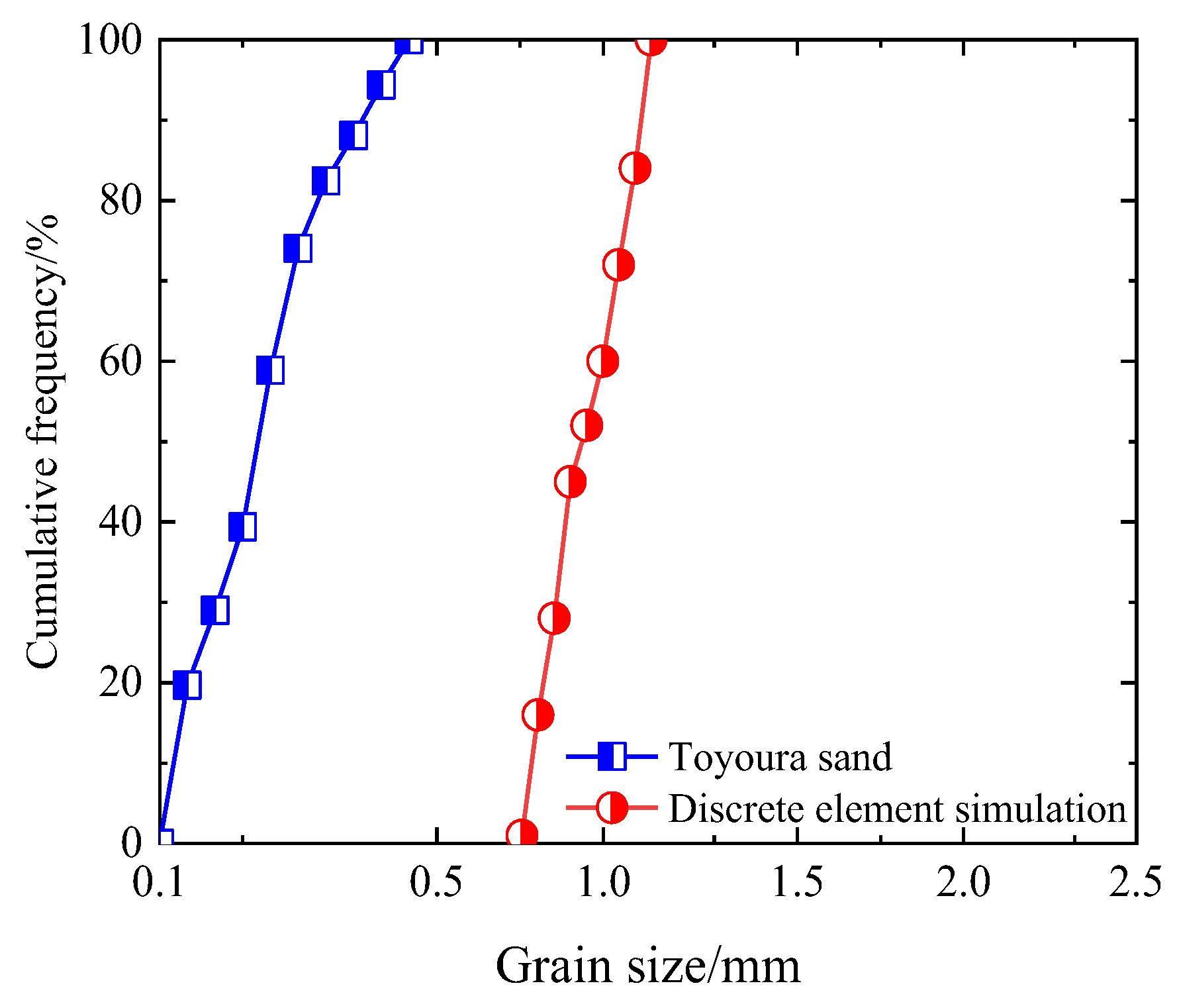
Within this investigation, the PFC 2D software version 5.0 is employed to simulate biaxial shear tests conducted on HBS. PFC 2D software is a discrete element simulation, which is a particle-level modeling. It can flexibly set the boundary conditions of biaxial shear tests, conduct multi-scale simulations from micro to macro, and visualize the simulation results to facilitate parameterization and sensitivity analysis. Compared with similar programs such as DEM (Discrete Element Method), it also has the advantages of multi-physics coupling, good flexibility and scalability, graphical interface, and visualization. The generated sediment specimen model in this paper takes the form of a rectangular structure with a height of 60 mm, a width of 30 mm, and an aspect ratio of 2.0. The actual sediment and hydrate particles exhibit intricate shapes and diminutive sizes. However, the higher the quantity of particles, the more complex their shapes, and the smaller their sizes in discrete element simulations, the higher the computational cost. In view of the consideration of limited computational resources, sediment particles, and hydrate particles are simplified to be simulated as disc particles in DEM simulation [26]. (Disc particles in discrete element simulations cannot be crushed during biaxial shear.) Notably, prior research conducted by Belheine et al. [36] and Evans et al. [37] demonstrated that scaling particle size in discrete element simulations effectively captures specimen mechanical behavior. In consideration of computational resource limitations, the discrete element specimens in this paper are also subjected to scaling. The grain sizes of sediments, ranging from 0.727 to 1.136 mm, are scaled based on the Toyoura sand grain size distribution [12], as depicted in Figure 1. Ding et al. [38] conducted a study revealing that in the two-dimensional filling process, a particle size ratio greater than 6.48 for the selected sand to hydrate allows hydrate particles to fill the tiniest pores in the sediments. Consequently, this study sets the particle size of hydrate particles to 0.1 mm (approximately one-seventh of the minimum sediment particle diameter).
HBS emerge via the orchestrated transport of methane gas via designated conduits into the pores of a shallow deep-sea soil framework with an initial bearing capacity. To better conform to the natural formation patterns of HBS, the model in this investigation triggers the generation of hydrate particles within the pores of consolidated sediments, following an isotropic consolidation pressure of 1 MPa. Moreover, due to the substantial disparity in particle size between hydrate and sediment particles, interparticle contact proves challenging, resulting in the suspension of numerous hydrate particles within the pore space of the sediments. In this simulation, an intricate methodology is employed to address this challenge. Initially, the particle size of sediment particles is expanded, and the pore space of the sediment is contracted, facilitating comprehensive contact among hydrate particles. Following the re-establishment of interparticle contacts, the sediment particles are then reverted to their original size. The detailed preparatory method is outlined as follows:
In the designated rectangular range, a sediment specimen lacking NGH is randomly generated based on the particle size grading curve depicted in Figure 3. The positions of the sediment particles are fixed, and their sizes are expanded, typically by a factor of 1.5. Following this, a consolidating pressure of 1 MPa is imposed to ensure the adequate consolidation of the sediment specimen. Simultaneously, hydrate particles are randomly generated in the pore space until it is entirely filled. If the generated particles fall short of meeting the required saturation degree, calculated by Equation (5), the particle size of sediment particles is reduced. This process is iterated until the sediment specimen achieves the desired saturation degree. The corresponding contact model is then established by defining contact points between particles. Specifically, the parallel adhesion model is employed between NGH particles and between NGH particles and sediment particles. Additionally, utilizing the rolling resistance model between sediment particles. The details of the contact model can be referenced from the literature [39]. To complete the specimen, flexible boundaries are constructed on both sides of the sediment specimen, as depicted in Figure 4. Subsequently, the immobilization of sediment particles is removed, and their diameters are restored to their original dimensions until all particles attain equilibrium.
where is the quantity of hydrate particles, Smh is the hydrate saturation of the HBS, A is the area of the rectangular sediment specimen, n is the porosity, and is the radius of the hydrate particles.
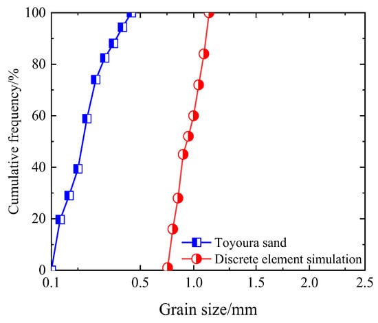
Figure 3.
Sand particle size distribution in Toyoura sand and discrete element simulation.
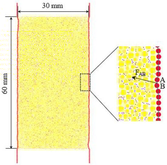
Figure 4.
Discrete element sample and mesostructured.
2.3. Flexible Boundary
In the practical implementation of biaxial shear tests on HBS, the specimen’s exterior is typically enveloped with a latex membrane to withstand circumferential pressure, while rigid loading plates are applied to the top and bottom surfaces to exert axial force. As illustrated in Figure 4, discrete element simulation software utilizes disc particles (membrane particles) with identical radii bonded to each other for constructing flexible boundaries. In this study, the radius of the membrane particles is set at 0.1 mm. The contact model between particles employs the linear contact bonding model, ensuring the transmission of force between membrane particles without torque. This configuration emulates the flexible pressurization role of the latex membrane in biaxial tests conducted in a chamber.
As the flexible boundary lacks the capability to maintain the target perimeter pressure value via servo control, unlike the rigid boundary, an equivalent concentrated force must be applied to each membrane particle on the flexible boundary to sustain the desired perimeter pressure. However, due to the linear contact bonding model connecting the membrane particles while undergoing the loading process, the position of the membrane particles changes with the loading and transmits force accordingly. Therefore, at each computational step, the real-time updating of the position of membrane particles is necessary to adjust the concentrated force applied to maintain the required target perimeter pressure for the simulation. Taking the example of two particles, A and B, as depicted in Figure 4, the contact between the particles is treated as a continuous membrane, and the length of the membrane corresponds to the contact length, denoted as L, which represents the distance between the centers of the two membrane particles. Hence, the force FAB applied to the flexible membrane can be expressed as follows:
where is the set target envelope pressure.
2.4. Mesoscale Parameters
2.4.1. Materials and Methods
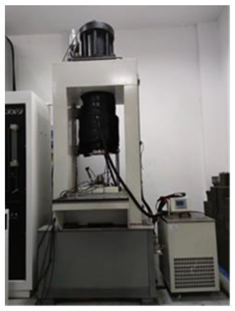
This article refers to the triaxial shear test scheme of HBS by Kajiyama et al. [40] and carries out biaxial verification tests of HBS specimens under different hydrate saturation and different confining pressure conditions. The experimental temperature is 4 °C. The average porosity of natural gas hydrate used was 32%, the average saturation was 38.7% and 54.3%, and the confining pressures selected were 1 MPa and 3 MPa, respectively. This test uses the KD-II high-pressure and low-temperature hydrate mechanical properties testing system of the School of Energy, Shandong University of Science and Technology (as shown in Figure 5). The experimental equipment includes fine sand, electronic scales, deionized water, methane gas, sample press, and constant temperature, constant humidity curing box (as shown in Figure 6), etc.
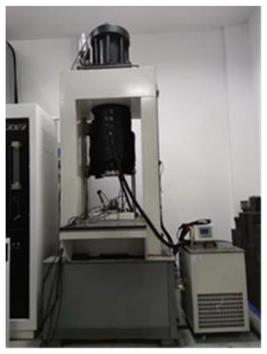
Figure 5.
KD-II-type high pressure and low temperature hydrate mechanical properties testing system.
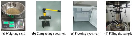
Figure 6.
Specimen preparation.
Before starting the test, clean the instrument and check the air tightness of the device. The specific test steps are as follows:
(1) Specimen preparation. The specific process (shown in Figure 6) is that first, the mass of the sand in the specimen is calculated to be 181.49 g based on the size of the specimen used in the test: Φ 50 mm × 100 mm and the porosity. And according to the particle size of sand, as shown in Figure 3, 181.49 g of sand is assigned. Then, according to the NGH saturation required for the test, the corresponding required deionized water volumes were calculated to be 24.19 mL and 33.94 mL, respectively. Mix the weighed sand and the measured deionized water evenly and put them into the mold. The layers are compacted to make a sand sample of the required size, and the prepared sand sample is placed in a constant temperature and humidity box (the temperature is set to −4 °C) and refrigerated for 24 h. Put the refrigerated specimen into a heat-shrinkable tube, install it in the triaxial pressure chamber, seal the upper and lower ends of the specimen with two O-rings, and calibrate the LVDT.
(2) Gas saturation method for the synthesis of NGH. Drop the confining pressure kettle, fill the pressure chamber with silicone oil, turn on the temperature control system, raise the temperature in the pressure chamber to 15 °C, and keep it for 30 min. After the ice in the test piece is completely melted, turn on the confining pressure controller to test, respectively. Apply peripheral pressures of 1 MPa and 3 MPa to the specimen, then set the confining pressure to tracking mode, and at the same time, open the air inlet valve and introduce methane gas into the specimen to increase the pore pressure. During this process, it is ensured that the peripheral pressure is always higher than the pore pressure, and the difference is the effective confining pressure. When the pore pressure reaches 10 MPa, close the air inlet valve. Then, the temperature of the pressure chamber is lowered from 15 °C to 4 °C via the temperature control system, so that the NGH can be fully synthesized in a low-temperature and high-pressure environment. When the pore pressure does not change, it is considered that the natural gas hydrate in the specimen has been fully synthesized.
(3) Loading process. The shear rate was set to 1 mm/min, and the test data were recorded every 2 s during the shearing process. The test was stopped when the strain of the specimen reached 15%.
(4) Unload the test piece. After the test is completed, the pressure in the system is safely released, the silicone oil in the confining pressure chamber is discharged into the oil cylinder, and the discharged gas is collected uniformly into the recovery device.
2.4.2. Mesoscopic Parameter Determination
In the realm of indoor experiments, the direct acquisition of mesoscale parameters such as the contact modulus, cohesion, and tensile strength of particles remains elusive. Furthermore, there is a current absence of reliable data pertaining to the contact bonding parameters specific to HBS. Consequently, the establishment of a correlation relating the mesoscale parameters of particles to the macroscopic mechanical parameters of HBS is of paramount significance. This study amalgamates results from indoor triaxial shear tests [40], referencing parameter values from prior research [21,41]. Employing the iterative “trial-and-error” approach, the mesoscale parameters of the contact bonds were meticulously fine-tuned in discrete element specimens. The contact modulus for the linear contact bonding model between membrane particles is precisely specified at 7 × 10⁶ Pa, representing the typical modulus of a latex membrane, while the strength is set at 1 × 10300 Pa to ensure the resilience of the flexible membrane during the loading process. Simultaneously, other mesoscale mechanical parameters of the particle and contact models are comprehensively detailed in Table 1 and Table 2.

Table 1.
Numerical model’s mesoscale parameters for particles.
Table 2.
Mesoscale parameters of the contact model in the numerical model.
The DEM to simulate the biaxial shear test of HBS is implemented as follows: Initially, a constant circumferential pressure is exerted onto the specimen of the hydrate deposit using a flexible boundary. Once the computational model achieves equilibrium, servo technology within PFC 2D is utilized to impose identical horizontal velocities (1 mm/min) on the upper and lower walls of the specimen, facilitating the application of axial load. The test is halted when the axial strain of the specimen reaches 15%.
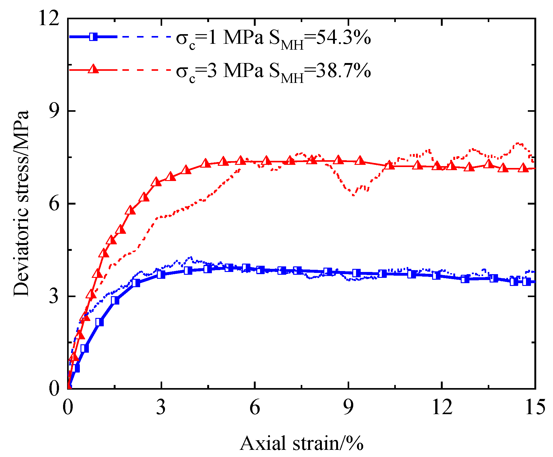
Figure 7 presents a comparative analysis between the outcomes of the discrete element simulation and the triaxial shear test. It is evident from the comparison that the numerical simulation in this study exhibits a commendable consistency with the results obtained from the indoor test. Therefore, the discrete element simulation utilized in this context adeptly captures the characteristics of HBS, rendering it a valuable tool for the scrutiny of their mechanical characteristics. The latter segment of the observed fluctuations in the stress–axial strain curves is more pronounced in this study. This intensity arises due to the compression process, wherein the increasing particle density leads to subtle displacements or misalignments, resulting in more noticeable fluctuations in the stress curves monitored on the observation wall.
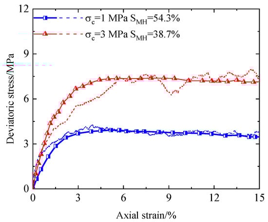
Figure 7.
Contrasting results from discrete element simulation with those from triaxial compression experimental.
2.5. Test Scheme
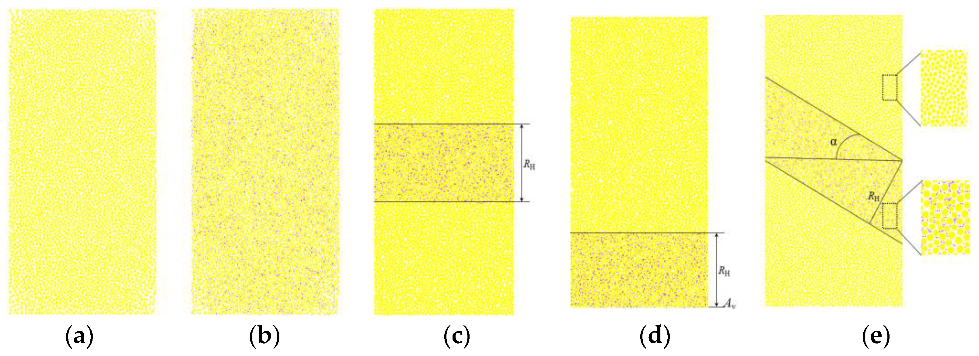
The distribution patterns of hydrates in the HBS specimens are illustrated in Figure 8. The numerical simulation comprises two sets of sediment specimens without hydrate layering distribution (Figure 8a,b) and three sets (Figure 8c–e) with distinct hydrate layering distribution patterns. These patterns involve parameters such as hydrate layer thickness RH, hydrate layer distribution position Ay, and the angle of the hydrate layer concerning the horizontal direction α. The specific simulation details are provided in Table 3. The HBS specimen is generated using the sampling method outlined in Section 2.2, with a hydrate saturation set to 50% (the typical range in the reservoir of the Nankai Trough of Japan is 40% to 80%). The surrounding pressure is set at 6 MPa [42]. The loading velocity is set at 1 mm/min, and the test concludes once the axial strain of the specimen hits 10%.
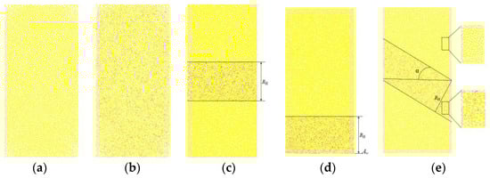
Figure 8.
Distribution patterns of hydrate in HBS specimen. (a) Sediment sample, (b) Sediment sample containing hydrate, (c) Sediment sample containing RH sediment with different hydrate layer thicknesses, (d) Ay sediment sample containing different hydrate layer positions, (e) Sediment sample containing different hydrate layer thicknesses. Hydrate layer inclination angle α sediment sample.
Table 3.
Simulation scheme.
3. Macroscale–Mesoscale Shear Mechanical Properties
3.1. Stress and Deformation Characteristics
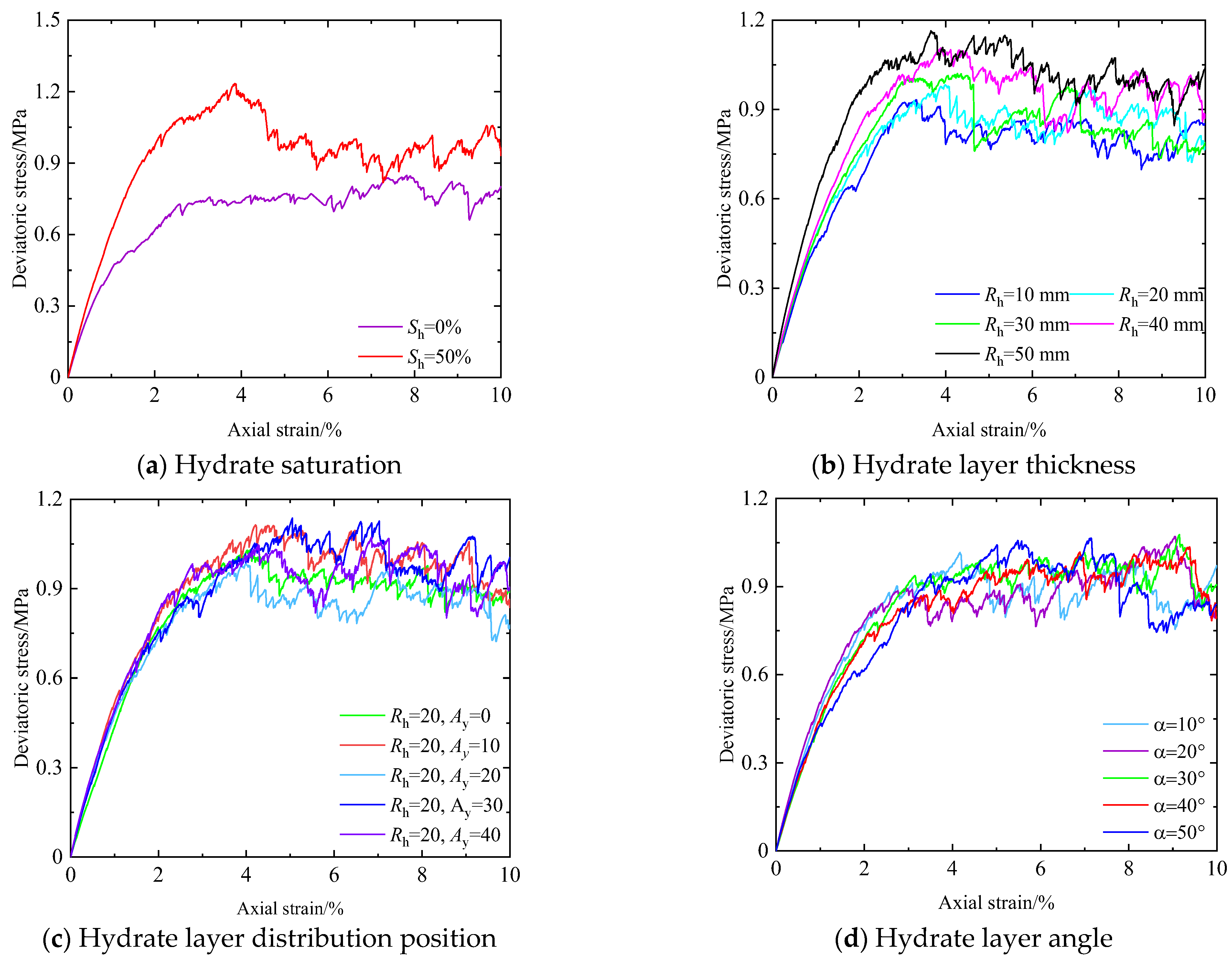
The stress–strain curves of HBS specimens exhibit varied distribution patterns, delineated in Figure 9. Notably, Figure 9a demonstrates that the stress curve corresponding to the specimen featuring 50% hydrate saturation has been above the stress curve of the specimen devoid of hydrate across the entire loading process. This disparity implies augmentation in the modulus of elasticity induced by the existence of hydrates. Moreover, the peak stress exhibited by the hydrate-containing specimen ascends appreciably, attributable to the bonding effect engendered between hydrate particles and sediment constituents. At the same time, specimens devoid of hydrate do not have a clear peak stress and a distinct post-peak phase in contrast to the presence of hydrate, and the stress–strain curves have transitioned from strain-softening to strain-hardening in specimens.
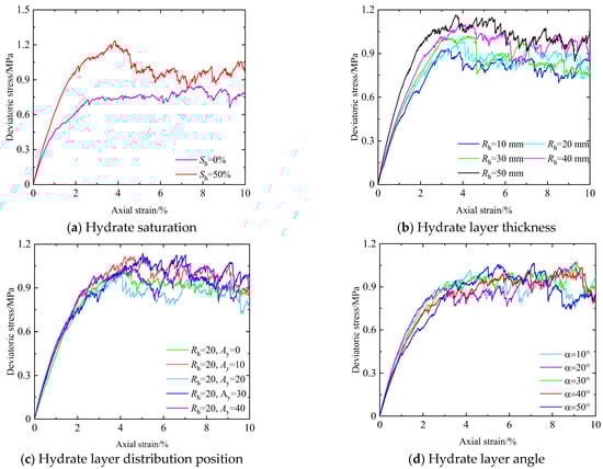
Figure 9.
Stress–strain curves of specimens with different hydrate distribution patterns.
The stress–strain curves, exemplified in Figure 9b, are greatly affected by the hydrate layer thickness on the HBS specimens. Notably, the curve has a discernible change rule that enlargement in RH leads to notable enlargement in peak strength alongside an increasingly pronounced strain-softening behavior within the specimens. This observed phenomenon can be attributed to distinct underlying mechanisms. At lesser RH, the prevailing interaction forces among sediment particles (primary effects are friction) and the concurrent presence of interparticle self-locking phenomena contribute to maintaining or even enhancing the overall strength of the specimen. This engenders an elevation in the specimen’s peak strength, while the strain-softening behavior is not obvious. Conversely, as the RH increases, the impact of the interparticle bonding breakdown on the corresponding stress–strain curve also intensifies. Moreover, the more the bonding is destroyed, the more the strength of the specimen decreases and the more noticeable the strain-softening behavior of the specimen is.
Delineated in Figure 9c, the strain-softening behavior of the specimen diminishes during the gradual movement of the hydrate layer from both ends of the specimen to the middle (Ay = 0, 40 mm → Ay = 20 mm). Notably, the specimen again shows obvious strain softening behavior when Ay = 20 mm. Because when the hydrate layer is confined to both ends of the specimen, the hydrate layer is directly affected by the axial load, and the interparticle bonding breaks down faster, consequently diminishing the specimen’s supporting capacity. However, as the hydrate layer is translocated toward the midsection, its upper and lower segments comprise loosely packed sediment particles. And the distal end, distanced from the primary axial load (far force end), inadequately transmits axial force to the hydrate layer, primarily burdening the section proximal to the axial load (near force end). This transmission, however, experiences attenuation due to the near force end’s influence on the sand layer, resulting in a deceleration of interparticle bonding destruction and, subsequently, a weakening of the strain-softening behavior of the specimen. Furthermore, at Ay = 20 mm, an obvious distinction arises from scenarios where the hydrate layer is solely present on one side of the specimen’s horizontal centerline. Here, the hydrate layer concurrently comes under axial loads at both ends and induces accelerated interparticle bonding destruction, consequently intensifying the strain-softening behavior of the specimen.
Specifically, the stress–strain curves of the specimens manifest evident strain softening behavior when α is equal to 10°, as depicted in Figure 9d. When α ≥ 20°, the stress–strain curve of the specimen shows obvious strain hardening behavior, and as the loading continues, the curve shows strain softening behavior. This is because the presence of α subjects the hydrate layer to uneven axial loading. The portion of the hydrate layer near the ends of the specimen experiences a greater influence from the axial load, leading to the initial breakdown of interparticle bonding. Conversely, the section farther from the ends is less affected. Under the influence of bonding between particles, the specimen retains a certain strength, resulting in a stress–strain curve exhibiting pronounced strain hardening behavior. However, as loading continues, extensive bonding breakdown occurs in the hydrate layer particles farther from the ends, causing the specimen to exhibit strain-softening behavior.
3.2. Strength Characteristics
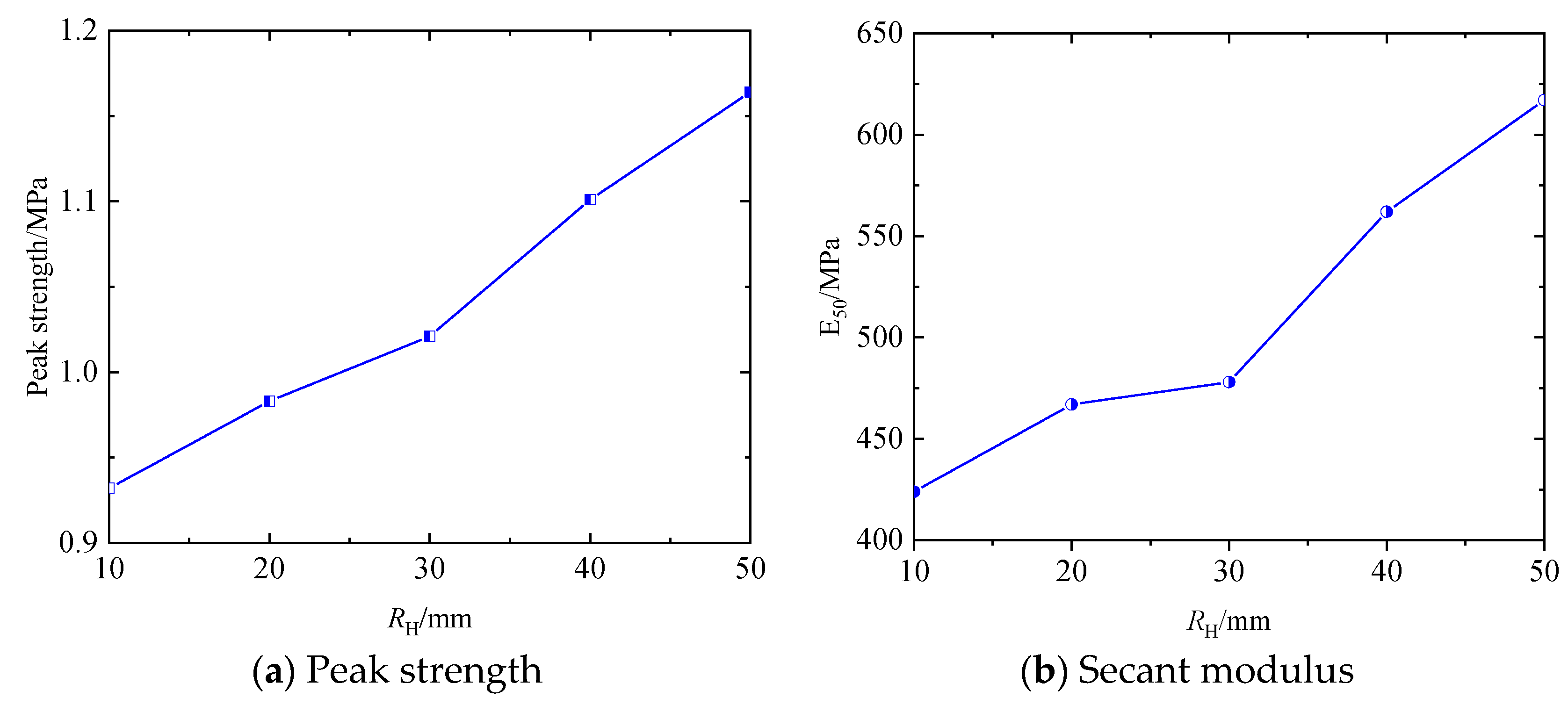
Figure 10 illustrates the variations curves in mechanical parameters of sediment specimens containing hydrate layers of varying thicknesses. Both the peak strength and the secant modulus E50 of the HBS (In this study, due to the inelastic nature of HBS, obtaining the initial modulus E0 encounters difficulty. In this test, the secant modulus E50 is employed to portray the stiffness of the specimen. E50 is defined as the incline from the origin to the point on the stress–strain curve corresponding to half of the ultimate strength.) exhibit a discernible increase relative to the RH. For instance, as RH escalates from 10 mm to 20 mm, the peak strength ascends from 0.932 MPa to 0.983 MPa (a 5% increase), while E50 rises from 424 MPa to 467 MPa (a 10% increase). Subsequently, with further increments in RH from 20 mm to 30 mm, the peak strength rises to 1.021 MPa (a 3.8% increase), accompanied by E50 reaching 478 MPa (a 2.3% increase). Similarly, elevating RH to 40 mm and 50 mm resulting in specimen strengths of 1.101 MPa and 1.164 MPa, along with E50 values of 562 MPa and 617 MPa, correlates with respective peak strength increments of 11.8% and 5.7%, the E50 increments of 5.7% and 9.8%. This is due to the fact that the larger the RH is, the stronger the bonding of the hydrate in the specimen is, subsequently augmenting shear capacity and resistance to deformation, resulting in a larger peak strength and E50 for the specimen.
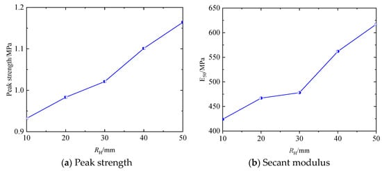
Figure 10.
Mechanical parameter curves of sediment specimens containing hydrate layers of different thicknesses.
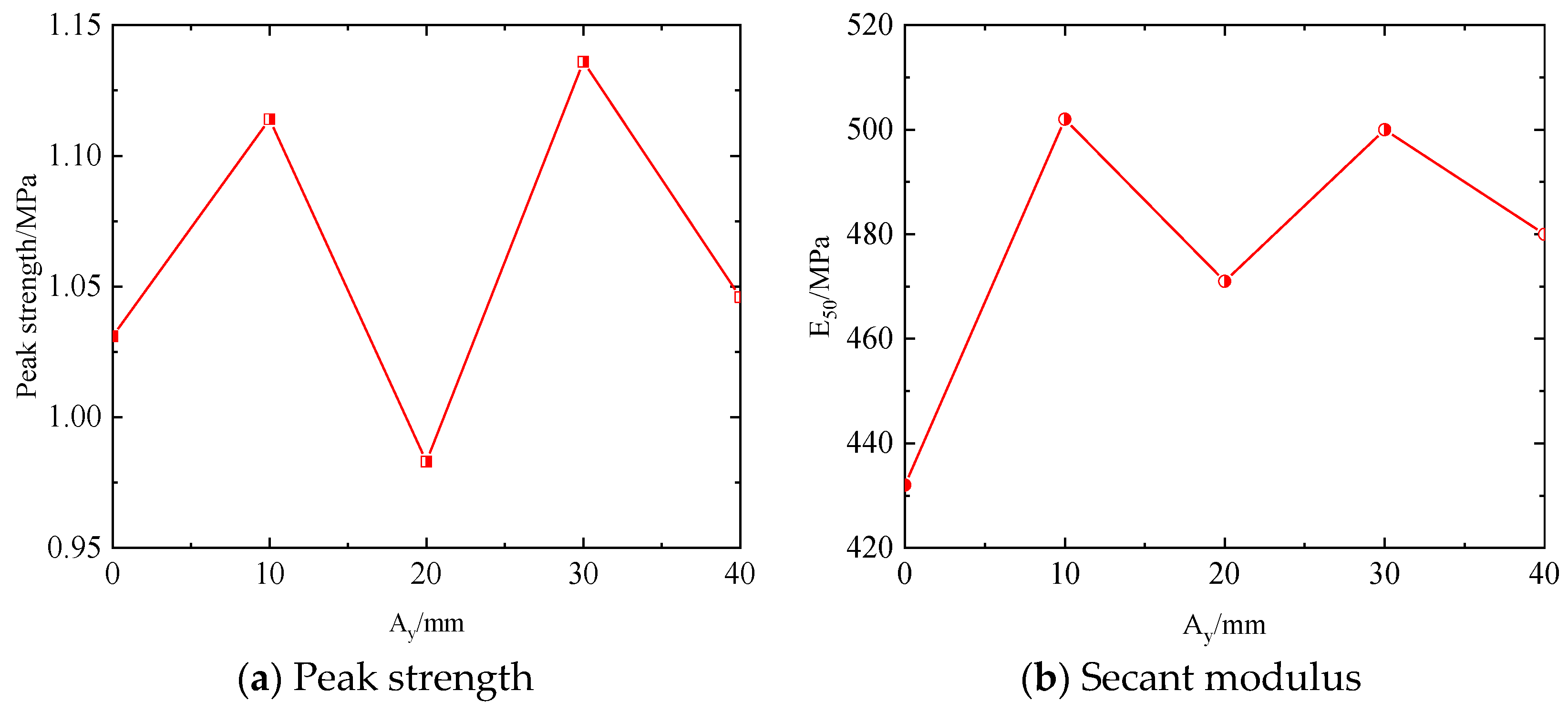
Figure 11 showcases the mechanical parameter curves of sediment specimens containing hydrate layers of different distribution positions. It can be seen that the demonstrates analogous mechanical parameter characteristics due to the symmetrical nature of the hydrate layer’s positioning at Ay = 0, 40 mm, and Ay = 10, 30 mm, thereby warranting only focus on the alterations observed when the hydrate layer resides at Ay = 0, 10, 20 mm. When the hydrate layer relocates from Ay = 0 mm to Ay = 10 mm, closer to the specimen’s center from the bottom, both the peak strength and E50 exhibit an increase. The peak strength elevates from 1.031 MPa to 1.114 MPa, increments of 8.1%, while E50 increases from 432 MPa to 502 MPa, increments of 16.2%. However, as the hydrate layer relocates from Ay = 10 mm to Ay = 20 mm, i.e., the hydrate layer changes from close to the middle of the specimen to the middle, both the peak strength and E50 witness a decline. Specifically, the peak strength reduces to 0.983 MPa, marking a 12.2% decrease, while E50 decreases to 471 MPa, marking a 6.2% decline. From the analysis of 3.1, the hydrate layer is in different positions, and the influence produced by the axial load is also different in size; it is evident that as the hydrate layer distances itself from the near force end, the impact of the axial load diminishes. Consequently, this results in a slower destruction of hydrate bonding, enhancing the specimen’s shear capacity and resistance to deformation. This, in turn, correlates with amplified peak strength and E50 values.
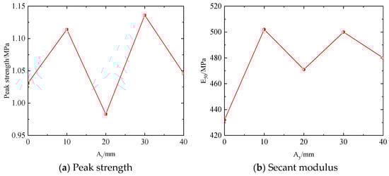
Figure 11.
Mechanical parameter curves of sediment specimens containing hydrate layers of different distribution positions.
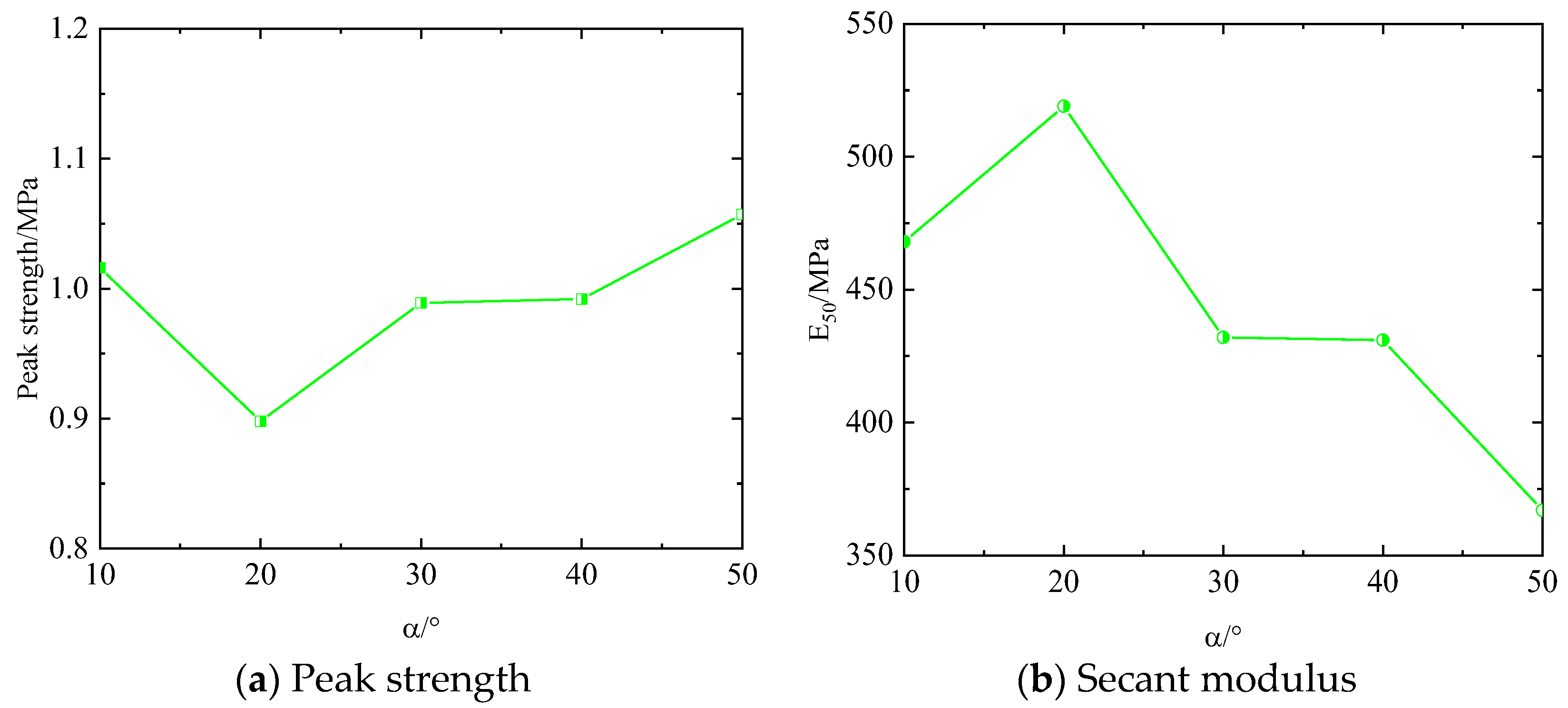
Figure 12 illustrates the mechanical parameter curves of sediment specimens containing hydrate layers of different angles. Distinct disparities in peak strength and the change in E50 are evident between α = 10° and α ≥ 20°. An analysis of Figure 9 and Figure 12 reveals that, at α = 10°, the stress–strain curve change rule of the specimen closely mirrors that of a horizontally placed hydrate layer. Conversely, for α ≥ 20°, an observable trend emerges wherein the peak strength of specimens elevates with increasing α, while E50 exhibits an overall declining trajectory with escalating α values. For instance, as α rises from 20° to 30°, the peak strength escalates from 0.898 MPa to 0.989 MPa, increments of 10.1%. In contrast, E50 experiences a substantial decline from 519 MPa to 412 MPa, a decrease of 20.7%. Similarly, as α increases from 30° to 40°, while no significant alteration occurs in the peak strength and E50. But as α increases from 40° to 50°, the peak strength increases to 1.057 MPa, representing a 6.9% increase. E50 experiences a substantial decline to 367 MPa, a decrease of 12.8%. This is because, with the increase in α, the enhanced bonding within the hydrate contributes to heightened shear resistance and increased peak strength. However, the presence of α in conjunction with axial loading introduces uneven stress distribution within the hydrate layer when the existence of α is not negligible. Consequently, sections closer to both ends of the specimen experience accelerated destruction of the bonding, resulting in reduced deformation resistance. So, the specimen’s E50 decreases as α increases.
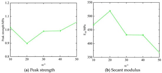
Figure 12.
Mechanical parameter curves of sediment specimens containing hydrate layers of different angles.
3.3. Typical Damage Law of HBS
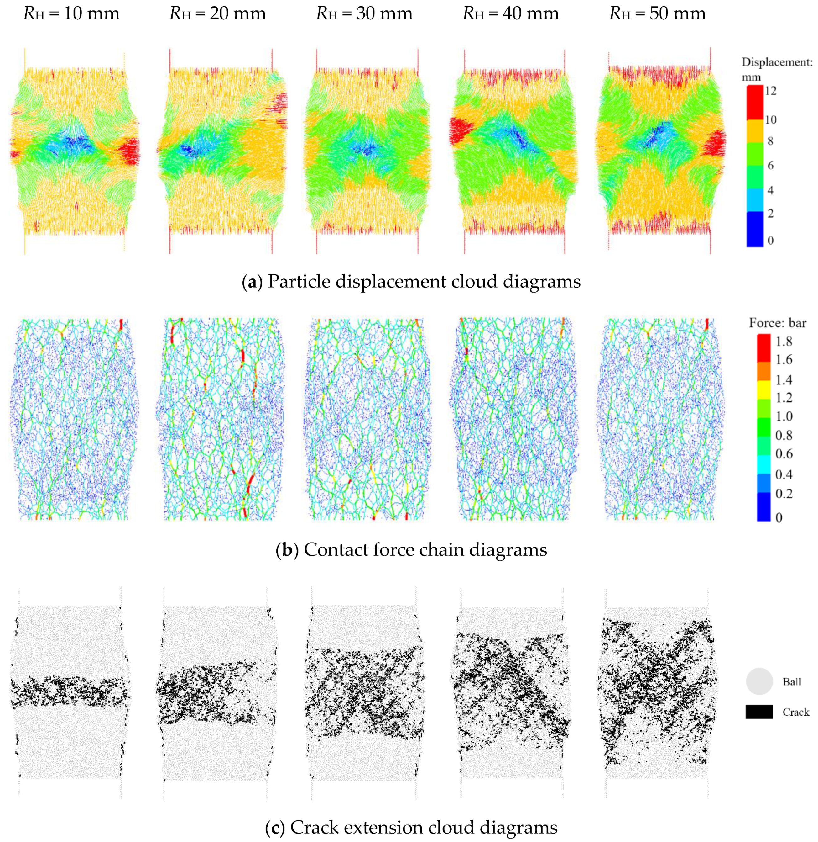
The deformation and damage processes within HBS are characterized by the development and change in deviatoric stress, axial strain and volumetric strain, and the emergence and progression of shear bands at the macroscale and mesoscale, respectively. Macroscopically, investigating the influence of axial load on the deformation and damage of HBS specimens needs to observe strain behavior rules such as axial strain and volumetric strain. Conversely, at the mesoscopic level, understanding the impact of axial load on the deformation of HBS specimens needs to examine particle displacement, the distribution of contact force chains, and the evolution of crack extension laws [27]. Specifically, Figure 13 illustrates typical damage law observed in sediment specimens containing hydrate layers of different thicknesses. The observations reveal the hydrate-free part exhibits considerable particle displacement, with most particles displaced between 6 and 8 mm (as shown in Figure 13a). It has significant differences in particle displacement (0~12 mm) of the hydrate layer, exhibiting a notable displacement gradient that facilitates shear band formation. This shear band represents a macroscopic manifestation of localized deformation characteristics within HBS. Furthermore, an increase in RH accentuates the rise of the shear band. This can be attributed to the shear band can be depicted as a region featuring active particle motion and substantial relative displacement at the mesoscopic level. As the shear strength of HBS amplifies, there is an increased demand for internal particle interaction forces to counteract deformation. Consequently, this necessitates a larger area of active particle motion, culminating in the more distinct manifestation of a pronounced shear band.
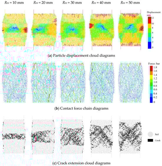
Figure 13.
Typical damage law of sediment specimen sediment containing hydrate layers of different thicknesses.
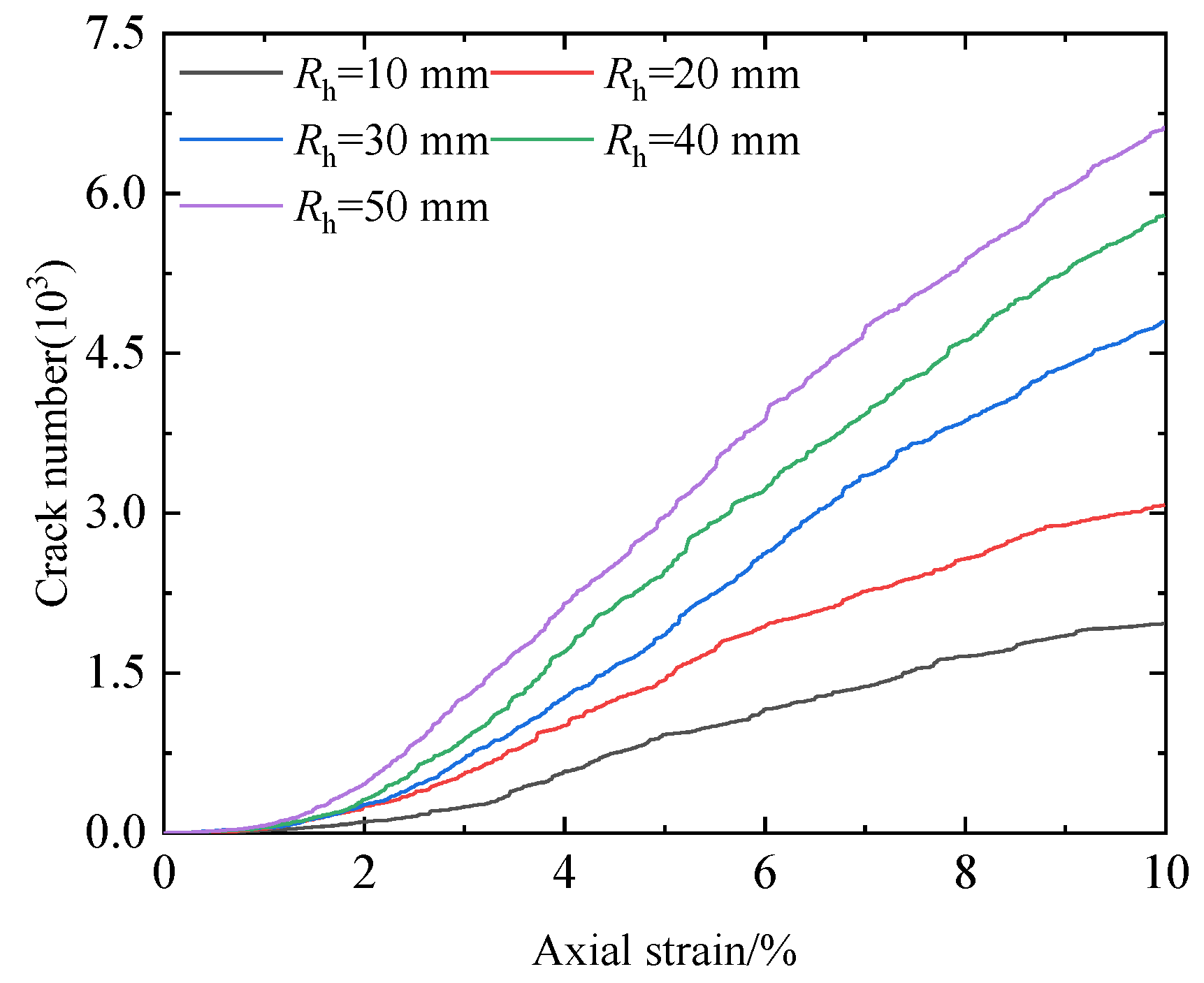
In Figure 13b, upon the transfer of contact forces from the hydrate-free portion to the hydrate layer within the specimen, noticeable deflection occurs in the strong force chain responsible for a larger force transmission. This deflection is particularly conspicuous within the hydrate layer, accentuating further with the increase in the RH. Additionally, in Figure 13c, observation from crack extension cloud diagrams demonstrates a direct relationship between increased RH and the formation of more pronounced shear bands. Correspondingly, higher RH values can result in heightening crack quantity near the shear bands, presenting a more regular distribution pattern of cracks. Moreover, the crack evolution law curves depicted in Figure 14 illustrate consistent trends across specimens containing hydrate layers of differing thicknesses, i.e., as the axial strain increases, the more the quantity of cracks, and the larger the RH is, the larger the crack rate is, and the more the quantity of cracks is.
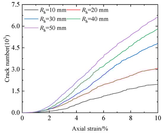
Figure 14.
Crack evolution law curves of sediment specimens containing hydrate layers of different thicknesses.
Figure 15 displays typical damage law observed in specimens featuring sediment from hydrate layers situated at varying distribution locations. Figure 15a and the corresponding contact force chain cloud diagrams (Figure 15b) illustrate intriguing observations during the progression from Ay = 0 mm to Ay = 10 mm and subsequently from Ay = 10 mm to Ay = 20 mm. Notably, the displacement gradient of particles within the specimen becomes progressively less pronounced during the Ay = 0 mm → Ay = 10 mm transition, accompanied by a gradual decline in the maximum value of the contact force chain within the hydrate layer (from 1.8 kN to 1.0 kN). Conversely, a contrasting trend emerges during the Ay = 10 mm → Ay = 20 mm transition, where the displacement gradient of particles becomes more apparent, accompanied by a gradual increase in the maximum value of the contact force chain within the hydrate layer (from 1.0 kN to 1.4 kN). From Figure 15c, it is noticeable that the displacement gradient of the hydrate layer in the specimen becomes more pronounced, resulting in a more distinct shear band formation. Moreover, in the vicinity of the shear band, the quantity of cracks increases, and their distribution becomes more regular.
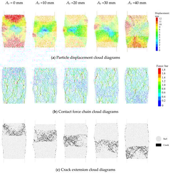
Figure 15.
Typical damage law of sediment specimens containing hydrate layers of different distribution positions.
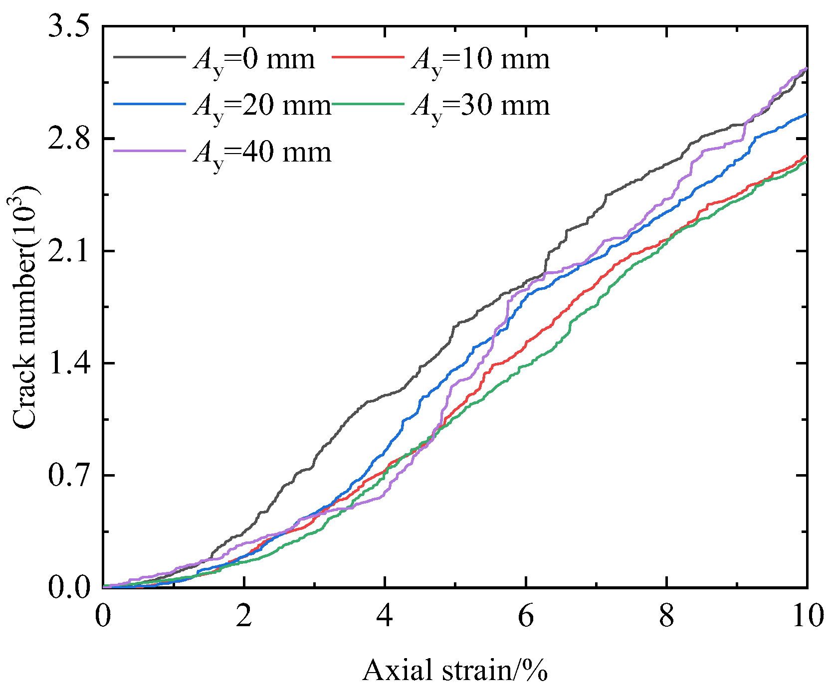
Simultaneously, by examining the crack evolution law curves presented in Figure 16 for the specimens, it becomes evident that specimens exhibiting diverse distribution locations exhibit analogous trends. Specifically, the crack rate and the number of cracks in the specimens display a decreasing tendency during the Ay = 0 mm → Ay = 10 mm phase. Subsequently, during the Ay = 10 mm → Ay = 20 mm phase, there is an observable increase in both the crack rate and the number of cracks in the specimens. In summary, the typical damage law observed in specimens containing hydrate layers of different distribution locations is intricately linked to the axial loads experienced by the hydrate layer at both the near and far force ends. And, as the axial load at the near force end increases, the particle displacement gradient within the specimen becomes more pronounced, leading to the conspicuous formation of shear bands. Moreover, the maximum value of the contact force chain experiences an elevation, resulting in a more regular distribution of cracks, a higher cracking rate, and an increased quantity of cracks.
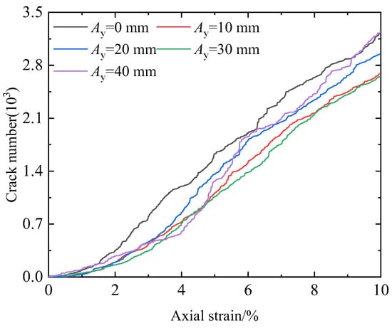
Figure 16.
Crack evolution of sediment specimens containing hydrate layers of different distribution positions.
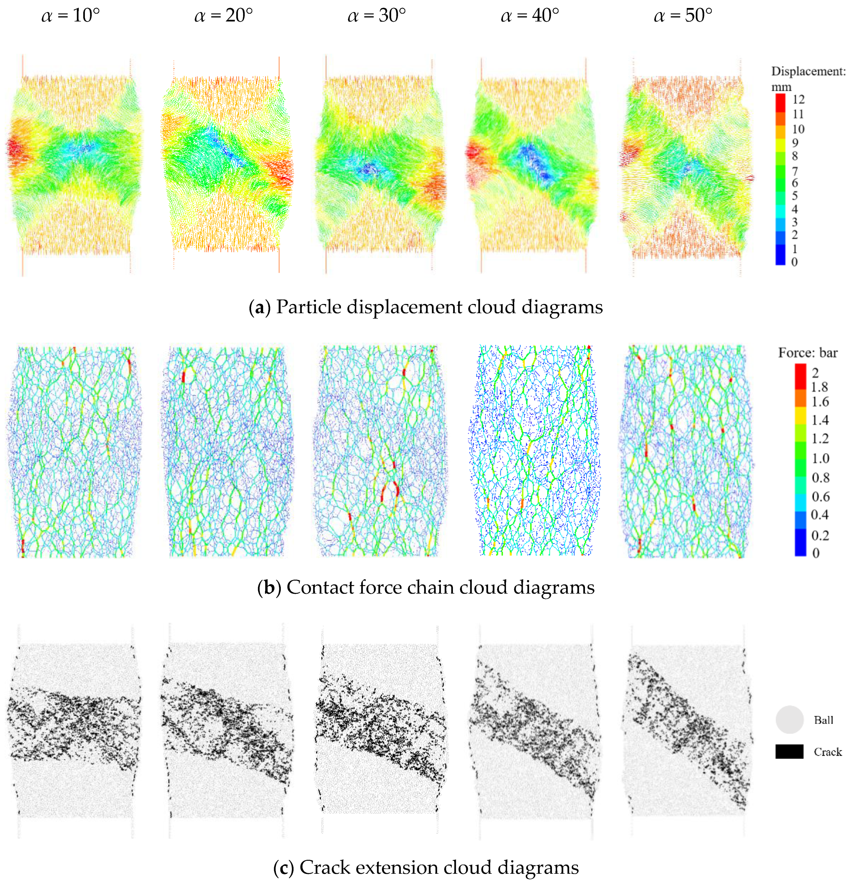
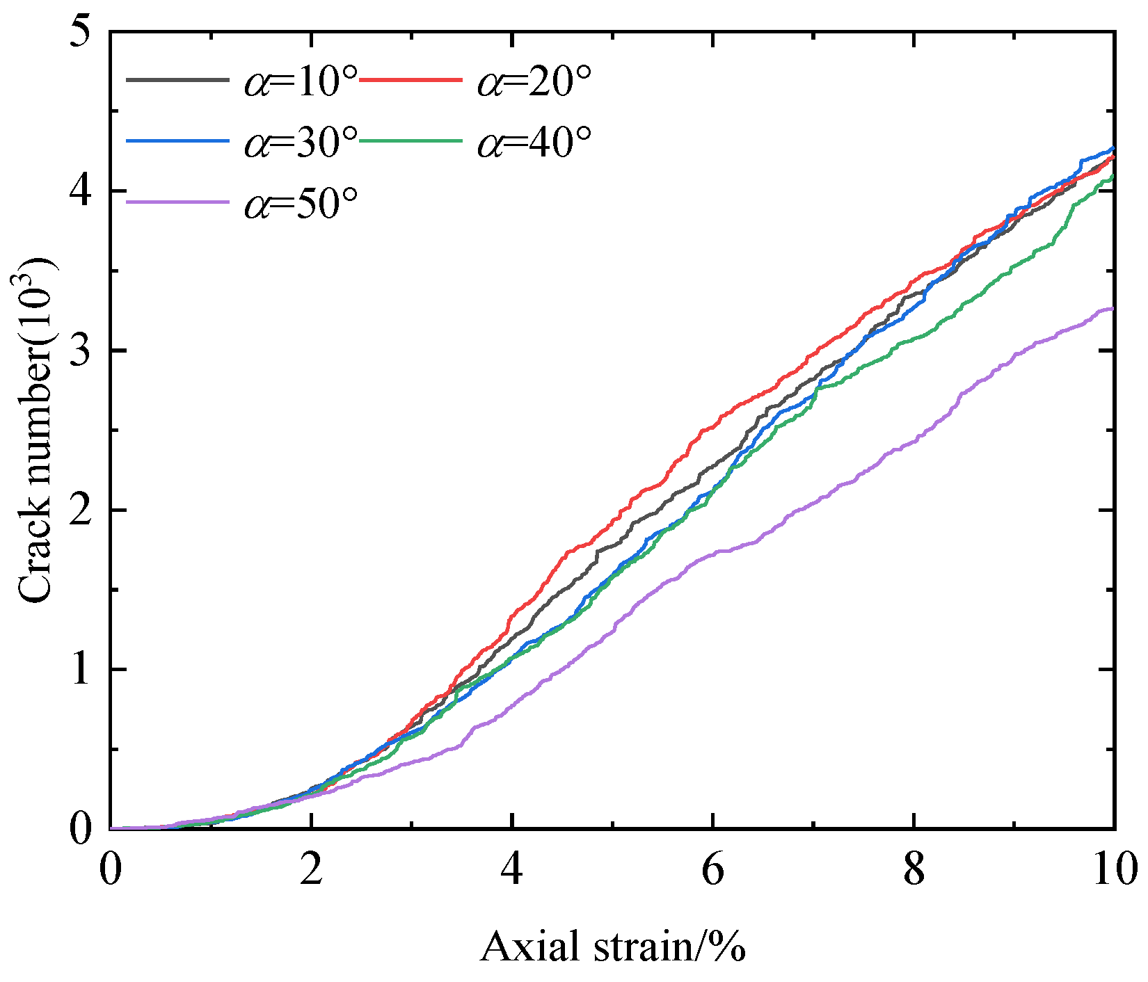
Analyzing the typical damage law of specimens containing hydrate layers of different angles reveals distinct displacement gradient regions within the specimens, basically overlapping with the hydrate layer, as shown in Figure 17. Concurrently, it is noticed that the particle displacement in the section of the hydrate layer proximal to the specimen ends surpasses that in the section distal to the ends. Furthermore, as the angle α increases, the portion of the hydrate layer distal to the specimen ends gradually exhibits concavity toward the inner region of the hydrate layer. Moreover, from Figure 17b and the corresponding crack extension diagrams (Figure 17c), it is evident that the portion of the specimen’s hydrate layer with higher contact force (proximal to the specimen ends) exhibits fewer cracks, while the section with lower contact force (distal to the specimen ends) shows a greater quantity of cracks. The aforementioned outcomes signify that the typical damage law of sediment specimens containing hydrate layers with different angles is closely related to the uneven distribution of axial pressure exerted on the hydrate layer. Furthermore, the sections of the hydrate layer experiencing greater axial load exhibit higher contact forces and a lower quantity of cracks. Moreover, from the crack evolution law curves of the specimens depicted in Figure 18, it is evident that the curves exhibit a similar trend. Specifically, the quantity of cracks increases with the rise in α. However, when α is less than 50°, the curves essentially overlap without significant differences due to the variation in angles. Nonetheless, at α equals 50°, there is a notable decrease in the number of cracks compared to the other four angles.
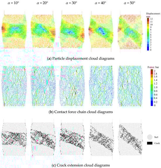
Figure 17.
Typical damage law of sediment specimens containing hydrate layers of different angles.
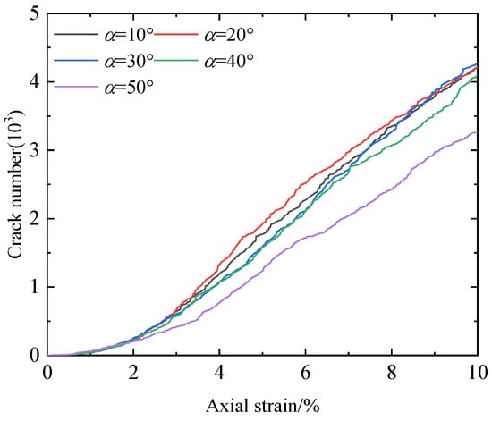
Figure 18.
Crack evolution of sediment specimens containing hydrate layers of different angles.
4. Conclusions
In this investigation, the discrete element simulation method is utilized to explore the shear mechanical characteristics at the macroscale and mesoscale in specimens containing hydrate-bearing sediment under different hydrate layering patterns, including hydrate layer thickness (RH), hydrate layer distribution position (Ay), and the angle between the hydrate layer and the horizontal direction (α). The following key conclusions are drawn:
(1) The strain-softening behavior of HBS specimens strengthens with the increase in RH, leading to higher peak strength and E50 values.
(2) Due to the presence of α, the stress–strain curve of HBS specimens exhibits significant strain hardening behavior, and as continued loading, the curve transitions to strain softening behavior.
(3) With the increase in RH, the formation of shear bands in specimens becomes more pronounced, accompanied by a higher quantity of cracks near the shear bands and a more regular distribution of cracks.
(4) During the process of Ay = 0 mm → Ay = 10 mm, the displacement gradient of particles in the specimen becomes less distinct, and the peak value of the contact force chain in the hydrate layer gradually decreases (1.8 kN → 1.0 kN).
(5) When α varies, the typical failure pattern of HBS specimens is closely related to the uneven forces exerted on the hydrate layer. The part of the hydrate layer experiencing a greater axial load exhibits larger contact forces and fewer cracks, while the part with a smaller axial load has smaller contact forces and a higher quantity of cracks.
Author Contributions
Funding acquisition, Y.J. and H.L.; conceptualization, Y.J. and M.L.; methodology, Y.J. and H.L.; data curation, X.D. and X.M.; writing—original draft preparation, X.D., M.L. and Y.S.; investigation, M.L. and P.Y.; resources, Y.J. and H.L.; writing—review and editing, P.Y. and H.L.; visualization, M.L. and X.M. All authors have read and agreed to the published version of the manuscript.
Funding
This research was funded by the Shandong Provincial Natural Science Foundation, China (ZR2019ZD14).
Institutional Review Board Statement
Not applicable.
Informed Consent Statement
Not applicable.
Data Availability Statement
Data associated with this research are available and can be obtained by contacting the corresponding author upon reasonable request.
Conflicts of Interest
Author M.L. was employed by the company China Minmetals Corporation. The remaining authors declare that the research was conducted in the absence of any commercial or financial relationships that could be construed as a potential conflict of interest.
References
- Kvenvolden, K.A. Methane hydrate-A major reservoir of carbon in the shallow geosphere. Chem. Geol. 1988, 71, 41–51. [Google Scholar] [CrossRef]
- Waite, W.F.; Santamarina, J.C.; Cortes, D.D.; Dugan, B.; Espinoza, D.N.; Germaine, J.; Jang, J.; Jung, J.W.; Kneafsey, T.J.; Shin, H.; et al. Physical properties of hydrate-bearing sediments. Rev. Geophys. 2009, 47, 465–484. [Google Scholar] [CrossRef]
- Chong, Z.R.; Yang, S.H.B.; Babu, P.; Linga, P.; Li, X.-S. Review of natural gas hydrates as an energy resource: Prospects and challenges. Appl. Energ. 2016, 162, 1633–1652. [Google Scholar] [CrossRef]
- Li, Y.; Wu, N.; Ning, F.; Gao, D.; Hao, X.; Chen, Q.; Liu, C.; Sun, J. Hydrate-induced clogging of sand-control screen and its implication on hydrate production operation. Energy 2020, 206, 118030. [Google Scholar] [CrossRef]
- Vedachalam, N.; Ramesh, S.; Jyothi, V.; Prasad, N.T.; Ramesh, R.; Sathianarayanan, D.; Ramadass, G.; Atmanand, M. Evaluation of the depressurization based technique for methane hydrates reservoir dissociation in a marine setting, in the Krishna Godavari Basin, east coast of India. J. Nat. Gas Sci. Eng. 2015, 25, 226–235. [Google Scholar] [CrossRef]
- Jin, G.; Xu, T.; Xin, X.; Wei, M.; Liu, C. Numerical evaluation of the methane production from unconfined gas hydrate-bearing sediment by thermal stimulation and depressurization in Shenhu area, South China Sea. J. Nat. Gas Sci. Eng. 2016, 33, 497–508. [Google Scholar] [CrossRef]
- Li, Y.; Liu, C.; Liao, H.; Dong, L.; Bu, Q.; Liu, Z. Mechanical properties of the mixed system of clayey-silt sediments and natural gas hydrates. Nat. Gas Ind. 2020, 40, 10. [Google Scholar] [CrossRef]
- Yan, P.; Luan, H.; Jiang, Y.; Yu, H.; Liang, W.; Cheng, X.; Liu, M.; Chen, H. Experimental Investigation Into Effects of Thermodynamic Hydrate Inhibitors on Natural Gas Hydrate Synthesis in 1D Reactor. Energy Technol. 2023, 11, 2300262. [Google Scholar] [CrossRef]
- Li, Y.; Wu, N.; Gao, D.; Chen, Q.; Liu, C.; Yang, D.; Jin, Y.; Ning, F.; Tan, M.; Hu, G. Optimization and analysis of gravel packing parameters in horizontal wells for natural gas hydrate production. Energy 2021, 219, 119585. [Google Scholar] [CrossRef]
- Li, Y.; Hu, G.; Wu, N.; Liu, C.; Chen, Q.; Li, C. Undrained shear strength evaluation for hydrate-bearing sediment overlying strata in the Shenhu area, northern South China Sea. Acta Oceanol. Sin. 2019, 38, 114–123. [Google Scholar] [CrossRef]
- Wu, Q.; Lu, J.S.; Li, D.L.; Liang, D.Q. Experimental study of mechanical properties of hydrate-bearing sediments during depressurization mining. Rock Soil Mech. 2018, 39, 4508–4516. [Google Scholar] [CrossRef]
- Hyodo, M.; Yoneda, J.; Yoshimoto, N.; Nakata, Y. Mechanical and dissociation properties of methane hydrate-bearing sand in deep seabed. Soils Found 2013, 53, 299–314. [Google Scholar] [CrossRef]
- Li, Y.; Dong, L.; Wu, N.; Nouri, A.; Liao, H.; Chen, Q.; Sun, J.; Liu, C. Influences of hydrate layered distribution patterns on triaxial shearing characteristics of hydrate-bearing sediments. Eng. Geol. 2021, 294, 106375. [Google Scholar] [CrossRef]
- Winters, W.; Waite, W.; Mason, D.; Gilbert, L.; Pecher, I. Methane gas hydrate effect on sediment acoustic and strength properties. J. Petrol. Sci. Eng. 2007, 56, 127–135. [Google Scholar] [CrossRef]
- Yoneda, J.; Masui, A.; Konno, Y.; Jin, Y.; Egawa, K.; Kida, M.; Ito, T.; Nagao, J.; Tenma, N. Mechanical behavior of hydrate-bearing pressure-core sediments visualized under triaxial compression. Mar. Petrol. Geol. 2015, 66, 451–459. [Google Scholar] [CrossRef]
- Luo, T.; Song, Y.; Zhu, Y.; Liu, W.; Liu, Y.; Li, Y.; Wu, Z. Triaxial experiments on the mechanical properties of hydrate-bearing marine sediments of South China Sea. Mar. Petrol. Geol. 2016, 77, 507–514. [Google Scholar] [CrossRef]
- Zhu, H.; Xu, T.; Xin, X.; Yuan, Y.; Jiang, Z. Numerical investigation of natural gas hydrate production performance via a more realistic three-dimensional model. J. Nat. Gas Sci. Eng. 2022, 107, 104793. [Google Scholar] [CrossRef]
- Bosikov, I.I.; Klyuev, R.V.; Silaev, I.V.; Pilieva, D.E. Estimation of multistage hydraulic fracturing parameters using 4D simulation. Gorn. Nauk. I Tekhnologii=Min. Sci. Technol. 2023, 8, 141–149. [Google Scholar] [CrossRef]
- Jiang, M.J.; Sun, Y.G.; Yang, Q.J. A simple distinct element modeling of the mechanical behavior of methane hydrate-bearing sediments in deep seabed. Granul. Matter. 2013, 15, 209–220. [Google Scholar] [CrossRef]
- Jiang, M.J.; Yu, H.S.; Harris, D. Bond rolling resistance and its effect on yielding of bonded granulates by DEM analyses. Int. J. Numer. Anal. Meth. Geomech. 2006, 30, 723–761. [Google Scholar] [CrossRef]
- Jiang, M.; Peng, D.; Ooi, J.Y. DEM investigation of mechanical behavior and strain localization of methane hydrate bearing sediments with different temperatures and water pressures. Eng. Geol. 2017, 223, 92–109. [Google Scholar] [CrossRef]
- Jiang, M.; Liu, J.; Kwok, C.Y.; Shen, Z. Exploring the undrained cyclic behavior of methane-hydrate-bearing sediments using CFD–DEM. Comptes Rendus Mécanique 2018, 346, 815–832. [Google Scholar] [CrossRef]
- Wang, H. Discrete Element Simulation Analysis of Mechanical Behavior of the Gas Hydrate-Bearing Sediments. Ijm 2018, 7, 85–94. [Google Scholar] [CrossRef]
- Yu, Y.; Cheng, Y.P.; Xu, X.; Soga, K. Discrete element modelling of methane hydrate soil sediments using elongated soil particles. Comput. Geotech. 2016, 80, 397–409. [Google Scholar] [CrossRef]
- Zhao, M.; Liu, H.; Ma, Q.; Xia, Q.; Yang, X.; Li, F.; Li, X.; Xing, L. Discrete element simulation analysis of damage and failure of hydrate-bearing sediments. J. Nat. Gas Sci. Eng. 2022, 102, 104557. [Google Scholar] [CrossRef]
- Jiang, Y.; Gong, B. Discrete-element numerical modelling method for studying mechanical response of methane-hydrate-bearing specimens. Mar. Georesour. Geotec. 2020, 38, 1082–1096. [Google Scholar] [CrossRef]
- Jiang, Y.; Li, M.; Luan, H.; Shi, Y.; Zhang, S.; Yan, P.; Li, B. Discrete Element Simulation of the Macro-Meso Mechanical Behaviors of Gas-Hydrate-Bearing Sediments under Dynamic Loading. Jmse 2022, 10, 1042. [Google Scholar] [CrossRef]
- Gong, B.; Jiang, Y.; Yan, P.; Zhang, S. Discrete element numerical simulation of mechanical properties of methane hydrate-bearing specimen considering deposit angles. J. Nat. Gas Sci. Eng. 2020, 76, 103182. [Google Scholar] [CrossRef]
- Dong, L.; Li, Y.; Liu, C.; Liao, H.; Chen, G.; Chen, Q.; Liu, L.; Hu, G. Mechanical Properties of Methane Hydrate-Bearing Interlayered Sediments. J. Ocean Univ. China 2019, 18, 1344–1350. [Google Scholar] [CrossRef]
- Zhou, M.; Soga, K.; Yamamoto, K. Upscaled Anisotropic Methane Hydrate Critical State Model for Turbidite Hydrate-Bearing Sediments at East Nankai Trough. J. Geophys. Res. Solid Earth 2018, 123, 6277–6298. [Google Scholar] [CrossRef]
- Brugada, J.; Cheng, Y.P.; Soga, K.; Santamarina, J.C. Discrete element modelling of geomechanical behaviour of methane hydrate soils with pore-filling hydrate distribution. Granul. Matter. 2010, 12, 517–525. [Google Scholar] [CrossRef]
- Kumar Saw, V.; Udayabhanu, G.N.; Mandal, A.; Laik, S. Methane Hydrate Formation and Dissociation in the presence of Bentonite Clay Suspension. Chem. Eng. Technol. 2013, 36, 810–818. [Google Scholar] [CrossRef]
- Zhou, Y.; Wei, C.F.; Zhou, J.Z.; Chen, P.; Wei, H.Z. Development and application of gas hydrate injection synthesis and direct shear test system. Rock Soil Mech. 2021, 42, 2311–2320. [Google Scholar] [CrossRef]
- Ai, J.; Chen, J.; Rotter, J.M.; Ooi, J.Y. Assessment of rolling resistance models in discrete element simulations. Powder Technol. 2011, 206, 269–282. [Google Scholar] [CrossRef]
- Shi, C.; Zhang, Q.; Wang, S. Numerical Simulation Technology and Application with Particle Flow Code (PFC5.0); China Architecture & Building Press: Beijing, China, 2018; p. 1. [Google Scholar]
- Belheine, N.; Plassiard, J.P.; Donzé, F.V.; Darve, F.; Seridi, A. Numerical simulation of drained triaxial test using 3D discrete element modeling. Comput. Geotech. 2009, 36, 320–331. [Google Scholar] [CrossRef]
- Evans, T.M.; Valdes, J.R. The microstructure of particulate mixtures in one-dimensional compression: Numerical studies. Granul. Matter. 2011, 13, 657–669. [Google Scholar] [CrossRef]
- Ding, Y.; Qian, A.; Lu, H.; Li, Y.; Zhang, Y. DEM investigation of the effect of hydrate morphology on the mechanical properties of hydrate-bearing sands. Comput. Geotech. 2022, 143, 104603. [Google Scholar] [CrossRef]
- Wang, H.; Zhou, Z.Y.; Zhou, B.; Xue, S.F.; Lin, Y.S. Impact of rolling resistance effect of particles on macro/micro mechanical properties of hydrate-bearing sediments. Acta Pet. Sin. 2020, 41, 885–894. [Google Scholar] [CrossRef]
- Kajiyama, S.; Wu, Y.; Hyodo, M.; Nakata, Y.; Nakashima, K.; Yoshimoto, N. Experimental investigation on the mechanical properties of methane hydrate-bearing sand formed with rounded particles. J. Nat. Gas Sci. Eng. 2017, 45, 96–107. [Google Scholar] [CrossRef]
- Ding, Y.; Qian, A.; Lu, H. Three-dimensional discrete element modeling of the shear behavior of cemented hydrate-bearing sands. J. Nat. Gas Sci. Eng. 2022, 101, 104526. [Google Scholar] [CrossRef]
- Colwell, F.; Matsumoto, R.; Reed, D. A review of the gas hydrates, geology, and biology of the Nankai Trough. Chem. Geol. 2004, 205, 391–404. [Google Scholar] [CrossRef]


Disclaimer/Publisher’s Note: The statements, opinions and data contained in all publications are solely those of the individual author(s) and contributor(s) and not of MDPI and/or the editor(s). MDPI and/or the editor(s) disclaim responsibility for any injury to people or property resulting from any ideas, methods, instructions or products referred to in the content. |
© 2023 by the authors. Licensee MDPI, Basel, Switzerland. This article is an open access article distributed under the terms and conditions of the Creative Commons Attribution (CC BY) license (https://creativecommons.org/licenses/by/4.0/).