Snapping Shrimp Noise Detection Based on Statistical Model

Abstract

Snapping Shrimps (SSs) live in a warm ocean except the North and South Poles, and they are characterized by generating strong shock waves underwater using large claws. Shock waves generated by these SSs are used for marine noise research as a signal and as a noise source, because they cause a decrease in the Signal-to-Noise Ratio (SNR), acting as one of the disruptors in fields such as sonar for target detection and underwater communication. A state-of-the-art technique to detect Snapping Shrimp Noise (SSN) is Linear Prediction (LP) analysis. Using the feature where SSN occurs for a very short time, the SSN interval was detected based on the phenomenon where the residuals appear large in the SSN interval when the LP analysis is used. In this paper, we propose an SSN interval detection technique using the Likelihood Ratio (LR) as a follow-up study to the LP-analysis-based method for further performance improvements. The proposed method was used to analyze the statistical distribution characteristics of the LP residual of SSNs compared to Gaussian, Laplace, and Gamma distributions through the Goodness-Of-Fit test. Based on this, the statistical-model-based LRs of the three distributions were computed to detect the SSN interval. Comparing the proposed method with the state-of-the-art method, the proposed method achieved 0.0620, 0.0675, and 0.0662 improvements in Gaussian, Laplace, and Gamma distributions in the Receiver Operating Characteristic curve and Area Under Curve, respectively. The study results confirmed that the proposed method can operate effectively in the marine acoustic environment. This can help find accurate intervals for the automatic labeling of or reduction in SSN.

1. Introduction

Snapping Shrimps (SSs) live in warm ocean areas except the North and South Poles, and they are located within $\pm 40°$ latitude [1,2,3]. This organism is characterized by having large claws, and when the claws are quickly closed for self-defense or to surprise or kill prey, bubbles are instantaneously generated by the water. When these bubbles expand and burst, a very powerful shock wave is generated [4]. These shock waves are generated for a very short time (less than 1 ms), and the sound source level at a distance of 1 m from the claws has been measured to be about 190 dB [5].

Acoustic research in the marine environment is influenced by various marine noises. Among them, Snapping Shrimp Noise (SSN) is used as a signal of interest for marine noise research in the marine environment because it is frequently generated and exhibits a frequency response in a wide band (60 Hz~250 kHz) [6]. It also acts as a major performance degradation factor by causing a decrease in the Signal-to-Noise Ratio (SNR) and it acts as a noise source within the ambient sound level in coastal seas [7,8]. Examples include areas such as human underwater communication [9,10], animal underwater communication [11], sonar signal processing [12,13], and target detection [14]. In particular, in the field of underwater communication, the bit error rate performance of orthogonal frequency division multiplexing systems may be severely degraded due to the influence of frequent SSN [10]. Since the SSN has adverse effects on the marine environments in most cases except studies on the sound of SSs themselves, research needs to be conducted to find an accurate SSN interval to reduce the impact of SSN and prevent system performance degradation.

Due to the above problems, research has been conducted continuously to detect SSN intervals and prevent performance degradation [15,16,17,18,19]. However, SSs are sensitive to the temperature of water, so it has the property of being affected by sunlight. Most of the SSN measurements are reported to have been made in very shallow waters [7]. Therefore, previous research may not reflect the impact on performance degradation occurring at deep depths. Recently, based on the Shallow-water Acoustic Variability Experiment 2015 (SAVEX 15) dataset [20], which recorded SSN from the East China Sea, off the coast of Jeju, Korea, from 14 to 28 May 2015, at a depth of about 100 m where sunlight does not reach into the marine environment, an algorithm has been proposed to detect the SSN interval by applying a cell average-CFAR (Constant False Alarm Rate) detector based on Linear Prediction (LP) analysis [21].

This paper proposes a method using the Likelihood Ratio (LR) based on statistical models to improve SSN interval detection performance in marine environments [22,23]. For this purpose, the SAVEX 15 dataset was used, and the Cumulative Distribution Function (CDF) of SSN and ambient noise modeled using the LP analysis method was obtained, because LP residuals of SSN have been proven effective in [21]. In order to carry out the Goodness-Of-Fit (GOF) test, the Kolmogorov–Smirnov (KS) test method was used. Afterwards, the similarity with Gaussian, Laplace, and Gamma distributions was compared through KS statistics [24]. Next, SSN intervals were detected by using statistical-model-based LRs. Finally, the performance of the proposed methods and the LP-analysis-based state-of-the-art method in [21] was compared using the Receiver Operating Characteristic (ROC) curve and Area Under Curve (AUC).

Glossary

(1)

$\mathrm{y}\left(\mathrm{n}\right)$: hydrophone input signal;

(2)

$\tilde{y}\left(n\right)$: estimated input signal based on LP analysis;

(3)

$S\left(n\right)$: SSN signal;

(4)

$\mathrm{v}\left(\mathrm{n}\right)$: ambient noise signal;

(5)

$\mathrm{e}\left(\mathrm{n}\right)$: LP residual signal;

(6)

$\mathrm{a}\left(\mathrm{l}\right)$: $l$-th linear coefficient;

(7)

$e_s\left(n\right)$: LP residual signal originating from SSN;

(8)

$e_v\left(n\right)$: LP residual signal originating from ambient noise.

2. Related Works

2.1. Linear Prediction Analysis

The hydrophone input signal $\mathrm{y}\left(\mathrm{n}\right)$ is expressed by the addition of the SSN $\mathrm{s}(\mathrm{n}$), which is the signal of interest, and the ambient noise $\mathrm{v}\left(\mathrm{n}\right)$ as shown in (1).

$$\mathrm{y}\left(\mathrm{n}\right)=s\left(n\right)+\mathrm{v}\left(\mathrm{n}\right),$$

(1)

where $\mathrm{n}$ indicates the sample index.

In addition, LP analysis is a technique for predicting the next sample using the linear weighted sum of the previous samples [25,26], and the estimated signal $\tilde{y}\left(n\right)$ for the input signal in (1) can be expressed by

$$\tilde{y}\left(\mathrm{n}\right)=\sum _{l=1}^{L}y\left(n-l\right)\mathrm{a}\left(\mathrm{l}\right),$$

(2)

where a$\left(\mathrm{l}\right)$ denotes the l-th linear coefficient, L is the order of LP coefficients, and an LP residual signal $\mathrm{e}\left(\mathrm{n}\right)$ can be defined as

$$e\left(n\right)=y\left(n\right)-\tilde{y}\left(n\right)=\mathrm{y}\left(\mathrm{n}\right)-\sum _{l=1}^{L}y\left(n-l\right)\mathrm{a}\left(\mathrm{l}\right).$$

(3)

In general, LP residuals of linearly predictable signals such as deterministic sinusoidal signals have values close to zero, but in the case of SSN, it has a non-stationary characteristic that occurs sporadically at a very high frequency; thus, it was confirmed that the error was large in the result obtained by LP analysis [21].

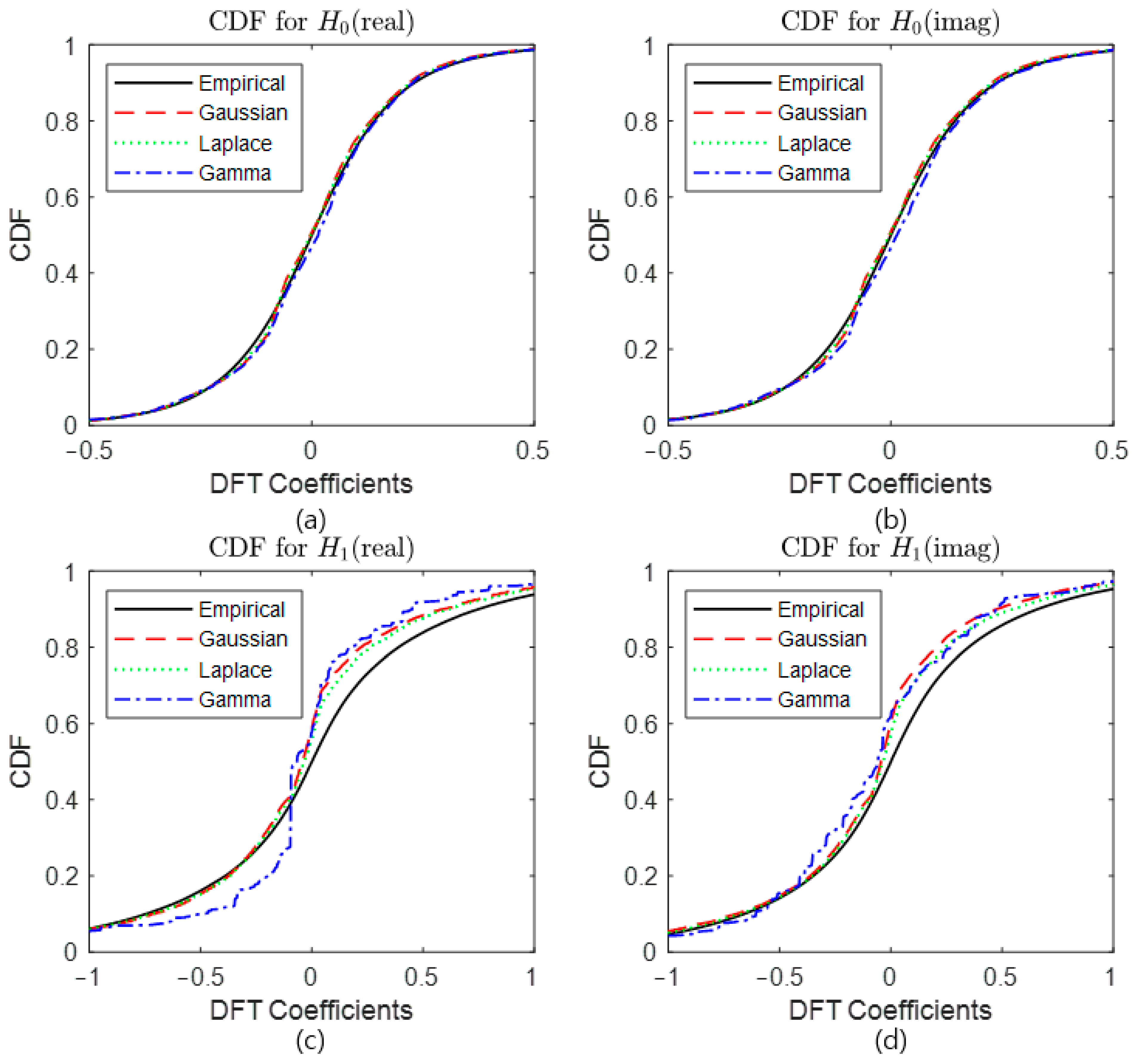
2.2. Goodness-of-Fit Test for Statistical Analysis

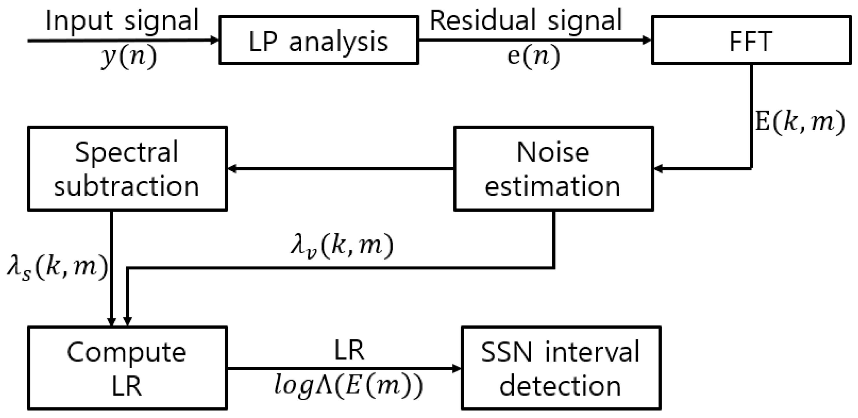
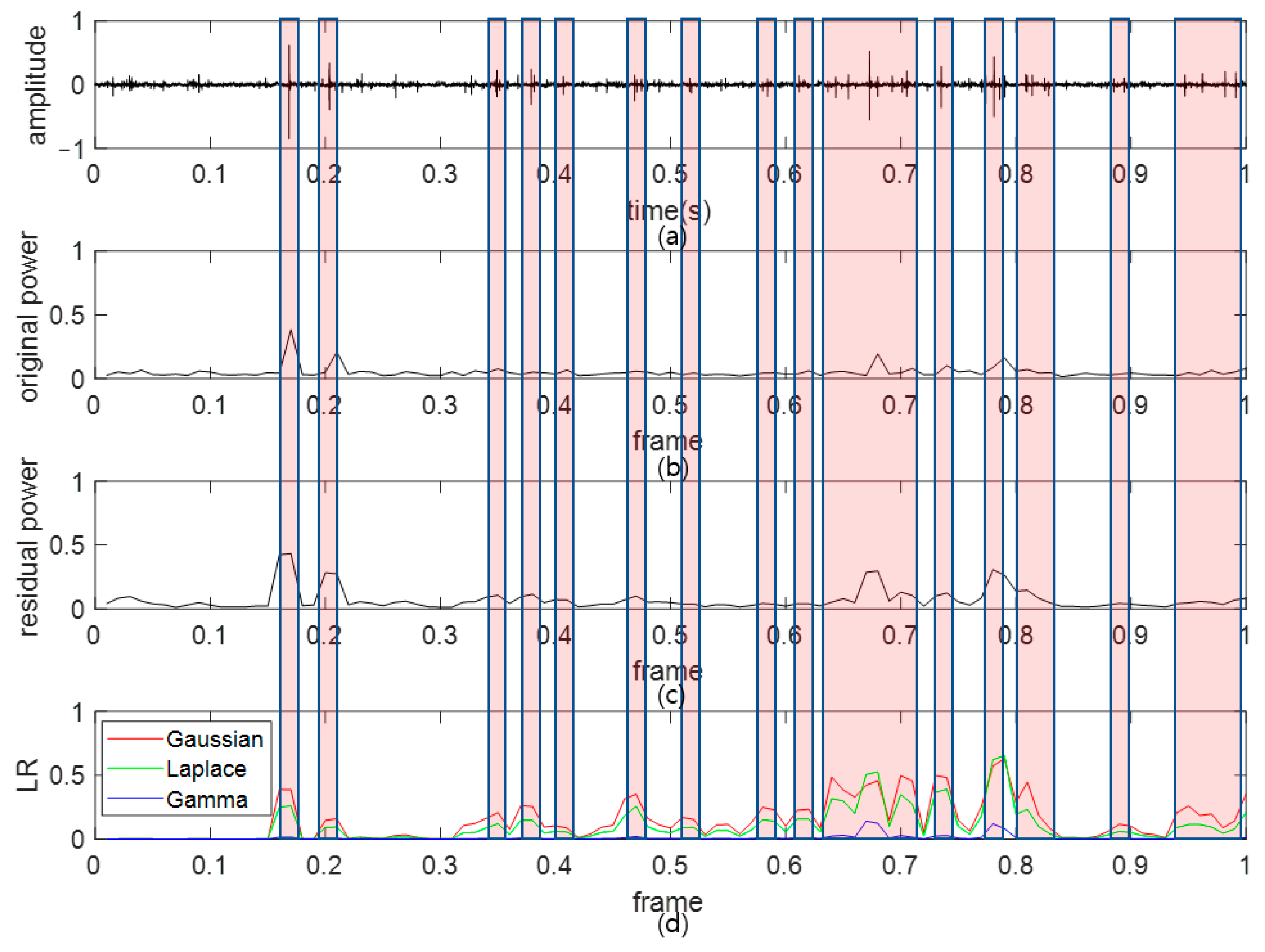
The KS test, known as the representative GOF test, is used to carry out a reliable analysis under each assumption [24]. The KS test is one of the nonparametric GOF test methods that can be used to evaluate the difference in the distribution of two probability distributions or sample data. It is mainly used to determine whether the two distributions are the same or to determine whether the distribution of sample data follows a particular distribution. Let X = {X₁,X₂, …, X_D}, which is all Discrete Fourier Transform (DFT) coefficients of a signal $\mathrm{x}\left(\mathrm{n}\right)\mathrm{i}\mathrm{n}\mathrm{a}\mathrm{s}\mathrm{c}\mathrm{e}\mathrm{n}\mathrm{d}\mathrm{i}\mathrm{n}\mathrm{g}\mathrm{o}\mathrm{r}\mathrm{d}\mathrm{e}\mathrm{r}$, which can be defined as in [27]

$$F_X\left(z\right)=\left\{\begin{array}{c}0,z<X_{\left(1\right)}\\ \frac{d}{D},X_{\left(d\right)}\le z<\\ 1,z\ge X_{\left(D\right)}\end{array}\right.X_{\left(d+1\right)},d=1,2,3,\dots D-1,$$

(4)

where X_(d), d = 1, …, D, are the order statistics of the data X and D is the total number of DFT coefficients used for the KS test. Next, to obtain KS statistics, we calculate the maximum measurement distance by subtracting the sample points of the parametric reference distribution $F$ from the sample points of the empirical distribution $F_X$:

$$T\left(\mathit{X}\right)=\underset{i}{\max }|F_X\left(X_i\right)-F\left(X_i\right)|.$$

(5)

A small KS statistic $T\left(\mathit{X}\right)$ indicates that the empirical distribution $F_X$ follows a specific reference distribution. In general, the KS test has the advantage that it does not rely on the size of the data for the GOF test.

3. Proposed Method

3.1. Signal Modeling Using the LP Residual Signal

The LP residual signal of SSN $\mathrm{e}\left(\mathrm{n}\right)$ in (3) can be defined as the sum of the LP residual originated from SSN $e_s\left(n\right)$ and ambient noise $e_v\left(n\right)$, as follows:

$$\mathrm{e}\left(\mathrm{n}\right)=\mathrm{y}\left(\mathrm{n}\right)-\tilde{y}\left(n\right)=e_s\left(n\right)+e_v\left(n\right).$$

(6)

Based on this, hypotheses $H_0$ and $H_1$ for the absence and presence of SSNs in $\mathrm{e}\left(\mathrm{n}\right)$, respectively, can be defined as

$$H_0:E\left(k,m\right)=E_v\left(k,m\right),$$

(7)

$$H_1:E\left(k,m\right)=E_s\left(k,m\right)+E_v\left(k,m\right).$$

(8)

where $E\left(k,m\right),E_s\left(k,m\right)$, and $E_v\left(k,m\right)$ represent the k-th frequency bin of the m-th frame of the LP, signal, and noise spectra, respectively.

3.2. Goodness-of-Fit Test for the LP Residual Signal

In order to apply an appropriate statistical model, a model close to the statistical distribution of $E_v(k,m)$ and the target signal $E_s\left(k,m\right)$ must be selected. In this paper, the representative Gaussian, Laplace, and Gamma distributions were considered for statistical modeling. First, by applying the Gaussian probability distribution, the spectral component distribution of the LP residual signals in $H_0$ and $H_1$ can be expressed as follows [22]:

$$P_G\left(E\left(k,m\right)|H_0\right)=\frac{1}{\pi {\lambda }_v(k,m)}·exp\left\{-\frac{\left|E\right(k,m){|}^2}{{\lambda }_v\left(k,m\right)}\right\},$$

(9)

$$P_G\left(E\left(k,m\right)|H_1\right)=\frac{1}{\pi \left({\lambda }_v\left(k,m\right)+{\lambda }_s\left(k,m\right)\right)}·exp\left\{-\frac{\left|E\right(k,m){|}^2}{{(\lambda }_v(k,m)+{\lambda }_s\left(k,m\right))}\right\},$$

(10)

where ${\lambda }_v(k,m)$ and ${\lambda }_s\left(k,m\right)$ represent the variances of $E_v(k,m)$ and $E_s\left(k,m\right)$, respectively.

Next, the spectral component distribution of the LP residual signals for the Laplace probability distribution is as follows:

$$P_L\left(E\left(k,m\right)|H_0\right)=\frac{1}{{\lambda }_v(k,m)}·exp\left\{-\frac{2\left(\right|E_{\left(R\right)}\left(k,m\right)|+|E_{\left(I\right)}\left(k,m\right)\left|\right)}{\sqrt{{\lambda }_v\left(k,m\right)}}\right\},$$

(11)

$$P_L\left(E\left(k,m\right)|H_1\right)=\frac{1}{{\lambda }_v\left(k,m\right)+{\lambda }_s\left(k,m\right)}·exp\left\{-\frac{2\left(\right|E_{\left(R\right)}\left(k,m\right)|+|E_{\left(I\right)}\left(k,m\right)\left|\right)}{\sqrt{{\lambda }_v\left(k,m\right)+{\lambda }_s\left(k,m\right)}}\right\}$$

(12)

where $E_{\left(R\right)}\left(k,m\right)$ and $E_{\left(I\right)}\left(k,m\right)$ denote the real and imaginary parts of $\mathrm{E}\left(\mathrm{k},\mathrm{m}\right)$, respectively.

Finally, the spectral component distribution of the LP residual signals for the Gamma probability distribution is as follows:

$$P_A\left(E\left(k,m\right)|H_0\right)=\frac{\sqrt{6}}{8\pi \sqrt{{\lambda }_v(k,m)}\left|E_{\left(R\right)}\left(k,m\right){|}^{0.5}\right|E_{\left(I\right)}\left(k,m\right){|}^{0.5}}·exp\left\{-\frac{\sqrt{3}\left(\right|E_{\left(R\right)}\left(k,m\right)|+|E_{\left(I\right)}\left(k,m\right)\left|\right)}{\sqrt{2}\sqrt{{\lambda }_v\left(k,m\right)}}\right\},$$

(13)

$$\begin{array}{ll}\hfill P_A\left(E\left(k,m\right)|H_1\right)& =\frac{\sqrt{6}}{8\pi \sqrt{{\lambda }_v\left(k,m\right)+{\lambda }_s\left(k,m\right)}\left|E_{\left(R\right)}\left(k,m\right){|}^{0.5}\right|E_{\left(I\right)}\left(k,m\right){|}^{0.5}}\hfill \\ & ·exp\left\{-\frac{\sqrt{3}\left(\right|E_{\left(R\right)}\left(k,m\right)|+|E_{\left(I\right)}\left(k,m\right)\left|\right)}{\sqrt{2}\sqrt{{\lambda }_v\left(k,m\right)+{\lambda }_s\left(k,m\right)}}\right\}.\hfill \end{array}$$

(14)

Based on the above three statistical models, the similarity of the distribution was confirmed using KS statistics. The results of the KS test of the experimental CDF and the presented distribution in the real and imaginary parts of noise and signals are summarized in Figure 1.

From

Table 1. The results of Kolmogorov–Smirnov test for the LP residual spectra of $H_0$ and $H_1$.

KS Statistics	${\mathit{H}}_0\left(\mathit{r}\mathit{e}\mathit{a}\mathit{l}\right)$	${\mathit{H}}_0\left(\mathit{i}\mathit{m}\mathit{a}\mathit{g}\right)$	${\mathit{H}}_1\left(\mathit{r}\mathit{e}\mathit{a}\mathit{l}\right)$	${\mathit{H}}_1\left(\mathit{i}\mathit{m}\mathit{a}\mathit{g}\right)$
Gaussian	0.0297	0.0260	0.1350	0.1396
Laplace	0.0214	0.0196	0.1007	0.1012
Gamma	0.0378	0.0477	0.1612	0.1295

, we found that the Laplace distribution has the smallest KS statistics among the three distributions. However, the difference is not that large compared to the other two, the Gaussian and Gamma distributions.

3.3. SSN Detection Using Likelihood Ratios

In order to utilize the statistical analysis for SSN detection, LRs of the three distributions are computed. In general, LR $\mathsf{\Lambda }\left(\mathrm{E}\left(\mathrm{k},\mathrm{m}\right)\right)$ for the k-th frequency bin can be defined by the ratio of the pdfs:

$$\mathsf{\Lambda }\left(\mathrm{E}\left(\mathrm{k},\mathrm{m}\right)\right)\equiv \frac{P\left(E\left(k,m\right)|H_1\right)}{P\left(E\left(k,m\right)|H_0\right)}.$$

(15)

Therefore, the LR for each Gaussian, Laplace, and Gamma distribution can be expressed by

$${\mathsf{\Lambda }}^G\left(E\left(k,m\right)\right)=\frac{P_G\left(E\left(k,m\right)|H_1\right)}{P_G\left(E\left(k,m\right)|H_0\right)}=\frac{1}{1+\xi (k,m)}·\exp \left\{\frac{\gamma \left(k,m\right)\xi \left(k,m\right)}{1+\xi \left(k,m\right)}\right\},$$

(16)

$$\begin{array}{ll}\hfill {\mathsf{\Lambda }}^L\left(E\left(k,m\right)\right)& =\frac{P_L\left(E\left(k,m\right)|H_1\right)}{P_L\left(E\left(k,m\right)|H_0\right)}\hfill \\ & =\frac{1}{1+\xi (k,m)}·\exp \left\{2\left(\left|E_{\left(R\right)}\left(k,m)\right|+{|E}_{\left(I\right)}\left(k,m\right)\right|\right)·\left(\frac{\sqrt{{\lambda }_v\left(k,m\right)+{\lambda }_s\left(k,m\right)}-\sqrt{{\lambda }_v\left(k,m\right)}}{\sqrt{{\lambda }_v\left(k,m\right)+{\lambda }_s\left(k,m\right)}\sqrt{{\lambda }_v\left(k,m\right)}}\right)\right\},\hfill \\ & \hfill \mathrm{a}\mathrm{n}\mathrm{d}\hfill \end{array}$$

(17)

$$\begin{array}{ll}\hfill {\mathsf{\Lambda }}^A\left(E\left(k,m\right)\right)& =\frac{P_A\left(E\left(k,m\right)|H_1\right)}{P_A\left(E\left(k,m\right)|H_0\right)}\hfill \\ & =\frac{1}{\sqrt{1+\xi (k,m)}}\hfill \\ & ·\exp \left\{\frac{\sqrt{2}}{\sqrt{3}}\left(\left|E_{\left(R\right)}\left(k,m)\right|+{|E}_{\left(I\right)}\left(k,m\right)\right|\right)·\left(\frac{\sqrt{{\lambda }_v\left(k,m\right)+{\lambda }_s\left(k,m\right)}-\sqrt{{\lambda }_v\left(k,m\right)}}{\sqrt{{\lambda }_v\left(k,m\right)+{\lambda }_s\left(k,m\right)}\sqrt{{\lambda }_v\left(k,m\right)}}\right)\right\}.\hfill \end{array}$$

(18)

where $\xi \left(k,m\right)$ is the $\mathrm{a}\mathrm{p}\mathrm{r}\mathrm{i}\mathrm{o}\mathrm{r}\mathrm{i}\mathrm{S}\mathrm{N}\mathrm{R}$ and $\gamma (k,m)$ is the $\mathrm{a}\mathrm{p}\mathrm{o}\mathrm{s}\mathrm{t}\mathrm{e}\mathrm{r}\mathrm{i}\mathrm{o}\mathrm{r}\mathrm{i}\mathrm{S}\mathrm{N}\mathrm{R}$ as follows:

$$\xi \left(k,m\right)=\frac{{\lambda }_s\left(k,m\right)}{{\lambda }_v\left(k,m\right)},$$

(19)

$$\gamma \left(k,m\right)=\frac{\left|E\right(k,m){|}^2}{{\lambda }_v\left(k,m\right)},$$

(20)

Taking the logarithm of (16)–(18), and calculating the mean of each log LR using all frequency bins of the m-th frame, we finally obtain

$$log\mathsf{\Lambda }\left(E\left(m\right)\right)=\frac{1}{K}\sum _{k=1}^{K}log\mathsf{\Lambda }\left(E\left(k,m\right)\right)$$

(21)

where K is the total number of frequency bins in a frame. The block diagram for the entire system of the proposed method is depicted in Figure 2.

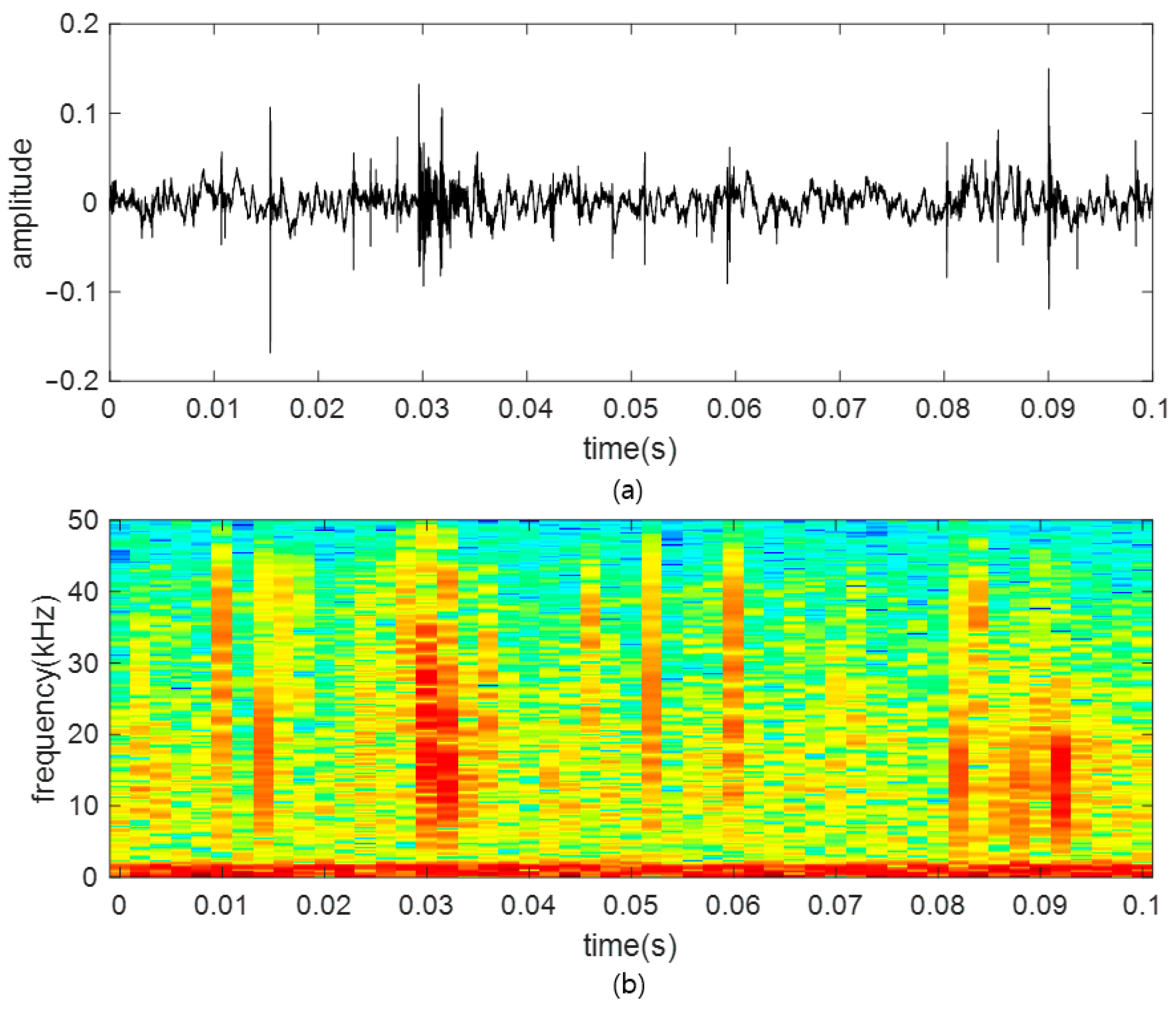
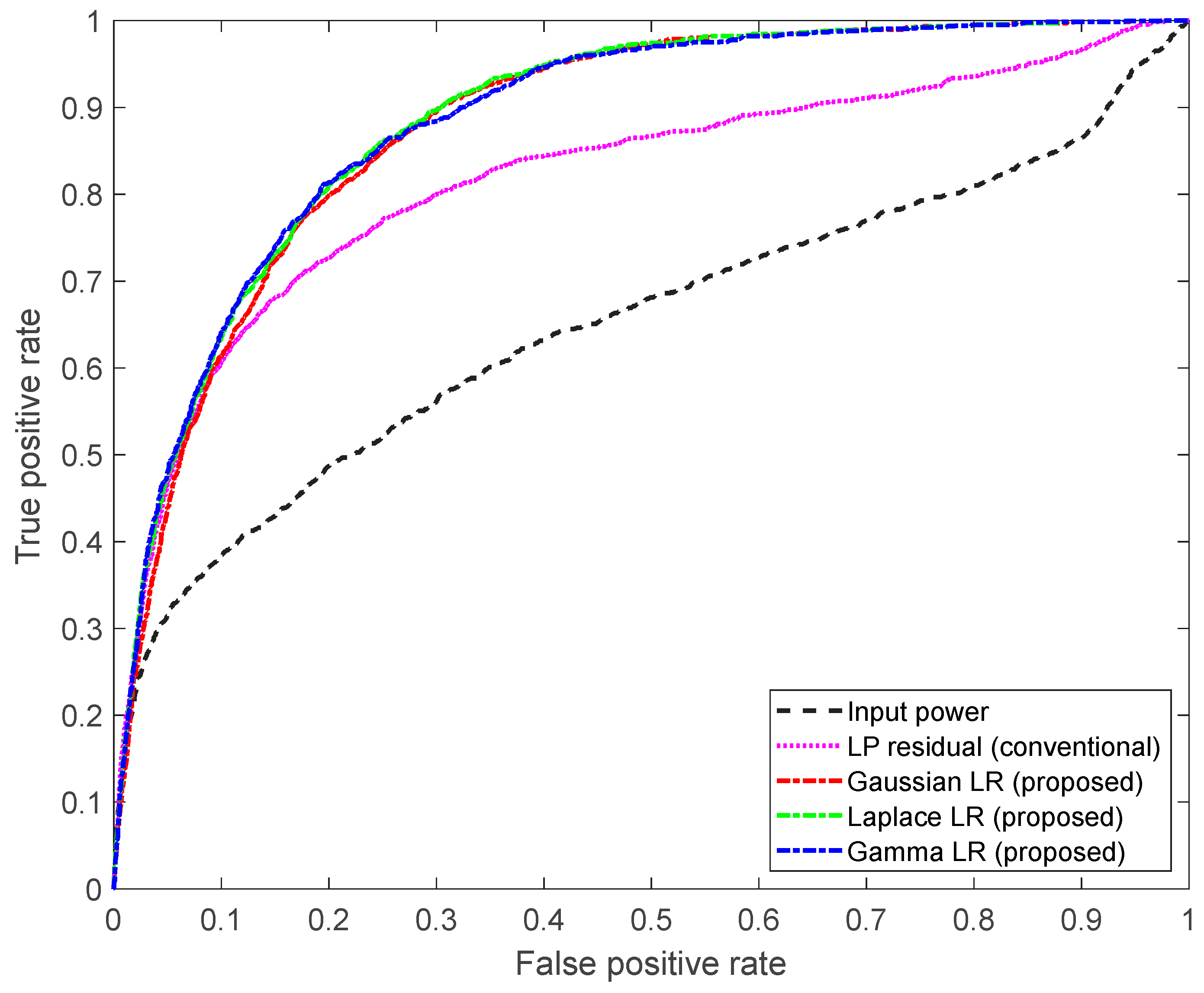
4. Experimental Results and Performance Assessment

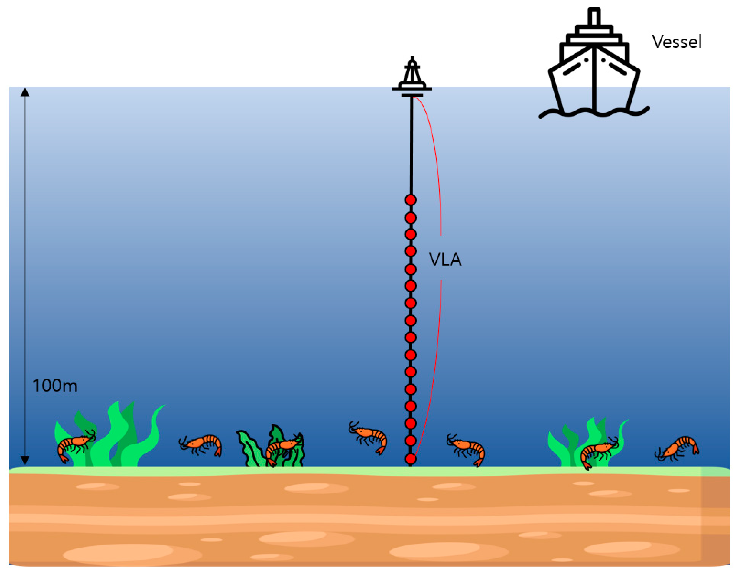
4.1. Experimental Environment

To evaluate the performance of the proposed method, we used the SAVEX 15 dataset collected from a real marine environment [20]. The SAVEX 15 was collected in the area of 32$°$30′ N 126$°$05′ E—32$°$35′ N 126$°$12′ E in East China Sea, off the coast of Jeju, Korea, from 14 to 28 May 2015; 16 hydrophones used a Vertical Line Array (VLA) set with 3.75 m intervals from 23.5 m to 79.75 m in depth; and the data were stored at a sampling frequency of 100 kHz. In order to evaluate the performance under identical conditions, 100 s of input samples, identical to [21], were used. For performance comparison, the LP-analysis-based method in [21] was compared, and the order of LP analysis was 20-th. The labels of SSN were manually marked from 100 s input samples, and the decision for SSN detection was performed every 10 ms. Throughout the process, the variance of the estimated ambient noise ${\lambda }_v\left(k,m\right)$ was obtained by Minima-Controlled Recursive Averaging (MCRA) [28], and the variance of the estimated SSN ${\lambda }_s\left(k,m\right)$ was calculated by using the spectral subtraction method [29]. Figure 3 presents the waveform and spectrogram of a part of the input samples (0.1 s), and the SAVEX 15 dataset collection environment is depicted in Figure 4.

4.2. Performance Evaluation

Figure 5 presents the results of the conventional and the proposed methods using a 1 s part of the input samples. As can be seen in Figure 5, both the conventional and proposed methods detect the SSN interval. However, the peak values of the conventional method tend to be low in some intervals, whereas the results of detecting the SSN interval using the proposed method show that the peak is more predominant on average than those of the conventional method.

In addition, the ROC curve and AUC were used for performance evaluation. The ROC curve is used to evaluate the performance of binary classification models and is a curve representing the change in the False Positive Rate (FPR) against he True Positive Rate (TPR) [30]. AUC means the area under the ROC curve, and as the value increases, the ability to minimize FPR while increasing TPR is outstanding, meaning that the model accurately distinguishes between positive and negative. The results of ROC curves and AUC are presented in Figure 6 and in

Table 2. The AUC results with ROC curve.

	Input Power	LP Residual [21]	Gaussian LR	Laplace LR	Gamma LR
AUC	0.6513	0.8182	0.8802	0.8857	0.8844

, respectively.

Looking at the results of the ROC curve, three curves of the proposed method are located in the upper left compared to the conventional method. In general, it represents a model with high TPR and low FPR at the same time. Therefore, it can be seen that the proposed method has improved performance compared to the conventional method. In the AUC, comparing this numerically, the conventional method [21] has a value of 0.8182, but it can be seen that the proposed method shows excellent performance with values of 0.8802 (Gaussian), 0.8857 (Laplace), and 0.8844 (Gamma). The AUC results show that the methods using LR are superior to the conventional method, and the performance of Laplace LR is the best. This result has a similarity with the KS statistics results in that the Laplace distribution recorded the minimum distance from the empirical distribution of the LP residual spectra in H₀ and H₁. Furthermore, it can be considered that the reason for the small difference between the Laplace LR and the other LRs originates from the sufficiently low values of the KS statistics of Gaussian and Gamma distributions.

5. Conclusions

In this paper, we proposed a technique for detecting the SSN interval using statistical-model-based LRs. For statistical modeling, the LP residual signal was obtained using an LP analysis method. The similarity between the CDF of the signal and noise components of LP residual spectra and the CDFs of Gaussian, Laplace, and Gamma distributions was compared through the KS test. As a result, the Laplace distribution had the lowest KS statistic among the three distributions. Subsequently, LRs based on the three distributions were derived and used for SSN detection. Compared to the state-of-the-art method using real ocean data, the proposed LR methods achieved performance improvements of 0.0620 (Gaussian), 0.0675 (Laplace), and 0.0662 (Gamma) in the ROC curve and AUC. Through the evaluation, it was confirmed that the proposed method had superior detection performance in the SSN interval compared to the conventional method. The results of this study confirmed that the proposed method can work effectively in the marine acoustic environment. This can help to find the exact interval for the automatic labeling of SSN intervals or noise reduction.

References

1. Johnson, M.W.; Everest, F.A.; Young, R.W. The role of snapping shrimp (Crangon and Synalpheus) in the production of underwater noise in the sea. Biol. Bull. 1947, 93, 122–138. [Google Scholar] [CrossRef] [PubMed]
2. Wicksten, M.K.; McClure, M.R. Snapping shrimps (Decapoda: Caridea: Alpheidae) from the Dampier Archipelago, western Australia. Rec. West. Aust. Mus. Suppl. 2007, 73, 61–83. [Google Scholar] [CrossRef]
3. Everest, F.A.; Young, R.W.; Johnson, M.W. Acoustical characteristics of noise produced by snapping shrimp. J. Acoust. Soc. Am. 1948, 20, 137–142. [Google Scholar] [CrossRef]
4. Versluis, M.; Schmitz, B.; Von der Heydt, A.; Lohse, D. How snapping shrimp snap: Through cavitating bubbles. Science 2000, 289, 2114–2117. [Google Scholar] [CrossRef] [PubMed]
5. Beng, K.T.; Teck, T.E.; Chitre, M.; Potter, J.R. Estimating the spatial and temporal distribution of snapping shrimp using a portable, broadband 3-dimensional acoustic array. In Proceedings of the Oceans 2003, Celebrating the Past… Teaming toward the Future (IEEE Cat. No. 03CH37492), San Diego, CA, USA, 22–26 September 2003; Volume 5, pp. 2706–2713. [Google Scholar]
6. Kim, B.N.; Hahn, J.; Cho, B.K.; Kim, B.C. Snapping shrimp sound measured under laboratory conditions. Jpn. J. Appl. Phys. 2010, 49, 07HG04. [Google Scholar] [CrossRef]
7. Lee, D.H.; Choi, J.W.; Shin, S.; Song, H.C. Temporal Variability in Acoustic Behavior of Snapping Shrimp in the East China Sea and Its Correlation With Ocean Environments. Front. Mar. Sci. 2021, 8, 779283. [Google Scholar] [CrossRef]
8. Lillis, A.; Mooney, T.A. Sounds of a changing sea: Temperature drives acoustic output by dominant biological sound-producers in shallow water habitats. Front. Mar. Sci. 2022, 9, 960881. [Google Scholar] [CrossRef]
9. Zhou, Y.; Wang, R.; Yang, X.; Tong, F. Orthogonal Projection and Distributed Compressed Sensing Based Impulsive Noise Estimation for Underwater Acoustic OSDM Communication. IEEE Internet Things J. 2023, 10, 22279–22293. [Google Scholar] [CrossRef]
10. Wang, S.; He, Z.; Niu, K.; Chen, P.; Rong, Y. New results on joint channel and impulsive noise estimation and tracking in underwater acoustic OFDM systems. IEEE Trans. on Wireless Commun. 2020, 19, 2601–2612. [Google Scholar] [CrossRef]
11. Au, W.W.; Banks, K. The acoustics of the snapping shrimp Synalpheus parneomeris in Kaneohe Bay. J. Acoust. Soc. Am. 1998, 103, 41–47. [Google Scholar] [CrossRef]
12. Loye, D.P.; Proudfoot, D.A. Underwater Noise to Marine Life. J. Acoust. Soc. Am. 1946, 18, 446–449. [Google Scholar] [CrossRef]
13. Kim, B.N.; Choi, B.K.; Kim, B.C.; Jung, S.K.; Park, Y.; Lee, Y.K. Seawater temperature and wind speeds dependences and diurnal variation of ambient noise at the snapping shrimp colony. In Proceedings of the IEEE 2012 Oceans, Yeosu, Republic of Korea, 21–24 May 2012; pp. 1–3. [Google Scholar]
14. Park, J.D.; Doherty, J.F. A steganographic app-roach to sonar tracking. IEEE J. Ocean. Eng. 2018, 44, 1213–1227. [Google Scholar] [CrossRef]
15. Tsihrintzis, G.A.; Nikias, C.L. Performance of optimum and suboptimum receivers in the presence of impulsive noise modeled as an alpha-stable process. IEEE Trans. Commun. 1995, 43, 904–914. [Google Scholar] [CrossRef]
16. Mahmood, A.; Chitre, M. Optimal and near-optimal detection in bursty impulsive noise. IEEE J. Ocean. Eng. 2017, 42, 639–653. [Google Scholar] [CrossRef]
17. Guimaraes, D.A.; Chaves, L.S.; de Souza, R.A.A. Snapping shrimp noise reduction using convex optimization for underwater acoustic communication in warm shallow water. In Proceedings of the ITS, Sao Paulo, Brazil, 17–20 August 2014; pp. 1–5. [Google Scholar]
18. Kim, H.; Seo, J.; Ahn, J.; Chung, J. Snapping shrimp noise mitigation based on statistical detection in underwater acoustic orthogonal frequency division multiplexing systems. Jpn. J. Appl. Phys. 2017, 56, 07JG02. [Google Scholar] [CrossRef]
19. Ahn, J.; Lee, H.; Kim, Y.; Chung, J. Snapping shrimp noise detection and mitigation for underwater acoustic orthogonal frequency division multiple communication using multilayer frequency. Int. J. Nav. Archit. Ocean Eng. 2020, 12, 258–269. [Google Scholar] [CrossRef]
20. Song, H.C.; Kim, S.M.; Kim, B.N.; Nam, S. Shallow-water acoustic variability experiment 2015 (SAVEX15) in the northern East China Sea. J. Acoust. Soc. Am. 2016, 140, 3012. [Google Scholar] [CrossRef]
21. Park, J.; Hong, J. Snapping shrimp noise detection methods based on linear prediction analysis. IEEE Sens. J. 2023; to be published. [Google Scholar] [CrossRef]
22. Chang, J.H.; Kim, N.S.; Mitra, S.K. Voice activity detection based on multiple statistical models. IEEE Trans. Signal Process. 2006, 54, 1965–1976. [Google Scholar] [CrossRef]
23. Kim, N.S.; Chang, J.H. Spectral enhancement based on global soft decision. IEEE Signal Process. Lett. 2000, 7, 108–110. [Google Scholar]
24. Glen, A.G.; Leemis, L.M.; Barr, D.R. Order statistics in goodness-of-fit testing. IEEE Trans. Reliab. 2001, 50, 209–213. [Google Scholar] [CrossRef]
25. Makhoul, J. Linear prediction: A tutorial review. Proc. IEEE 1975, 63, 561–580. [Google Scholar] [CrossRef]
26. Hayes, M.H. Statistical Digital Signal Processing and Modeling; John Wiley & Sons: Hoboken, NJ, USA, 1996. [Google Scholar]
27. Reininger, R.; Gibson, J. Distributions of the two dimensional DCT coefficients for images. IEEE Trans. Commun. 1983, 31, 835–839. [Google Scholar] [CrossRef]
28. Cohen, I.; Berdugo, B. Noise estimation by minima controlled recursive averaging for robust speech enhancement. IEEE Signal Process. Lett. 2002, 9, 12–15. [Google Scholar] [CrossRef]
29. Boll, S. Suppression of acoustic noise in speech using spectral subtraction. IEEE Trans. Acoust. Speech Signal Process. 1979, 27, 113–120. [Google Scholar] [CrossRef]
30. Hanley, J.A.; McNeil, B.J. The meaning and use of the area under a receiver operating characteristic (ROC) curve. Radiology 1982, 143, 29–36. [Google Scholar] [CrossRef]
Figure 1. The empirical CDF for LP residual spectra of ambient noise and SSN: (a) real parts of the ambient noise, (b) imaginary parts of the ambient noise, (c) real parts of the SSN, (d) imaginary parts of the SSN.
Jmse 12 00042 g001
Figure 2. The block diagram of proposed method.
Jmse 12 00042 g002
Figure 3. Part of the input sample SAVEX 15 data: (a) waveform, (b) spectrogram (where the peak values in (a) and the dark red parts of (b) are considered SSN).
Jmse 12 00042 g003
Figure 4. The SAVEX 15 dataset collection environment.
Jmse 12 00042 g004
Figure 5. The contour of the normalized conventional LP analysis based method and proposed method LRs: (a) original input signal, (b) input signal power, (c) LP residual (conventional), (d) proposed LRs (red: Gaussian, green: Laplace, blue: Gamma).
Jmse 12 00042 g005
Figure 6. ROC curve comparison of input power, LP residual (conventional), and proposed LRs (red: Gaussian LR, green: Laplace LR, blue: Gamma LR).
Jmse 12 00042 g006