Numerical Simulation Study of Seafloor Hydrothermal Circulation Based on HydrothermalFoam: A Case Study of the Wocan-1 Hydrothermal Field, Carlsberg Ridge, Indian Ocean

Abstract

Deep-sea hydrothermal circulation plays a pivotal role in the material and energy exchange in deep-sea environments, exerting significant influence on the evolution of seawater chemistry and global climate dynamics. Based on existing data and assumptions, this study presents a numerical model tailored for the hydrothermal circulation in the Wocan-1 Hydrothermal Field, Carlsberg Ridge, Indian Ocean. The model successfully simulates the hydrothermal circulation patterns within the oceanic crust, providing detailed insights into temperature distribution, flow field structures, and elemental concentration gradients. Through data analysis of the simulation results, we inferred the depth and temperature of potential heat sources within the Wocan-1 hydrothermal field. The maximum temperature of the heat source T_max = 823K (550 °C) and the depth of the heat source h = 1 km are possible results. To deepen understanding of the heat source’s impact on fluid temperatures, a sensitivity analysis was conducted. The findings show a positive correlation between both the heat source’s temperature and its depth with the fluid temperature at vent outlets. Regarding elemental transport, this paper offers a preliminary exploration of the kinetic processes in hydrothermal circulation and presents an empirical relationship linking elemental concentrations at the bottom to those at the vent: C_vent = 0.26 C_boundary. This study enhances current numerical models for hydrothermal vents, offering valuable insights for future work and utilization in the Wocan-1 hydrothermal field, and potentially in any other hydrothermal field.

1. Introduction

Hydrothermal circulation beneath the seafloor plays a pivotal role in facilitating the exchange of energy and mass among the lithosphere, hydrosphere, and biosphere, contributing to 20–25% of the global heat flux [1]. This process is integral to Earth’s geochemical recycling [2]. The efflux from hydrothermal vents, characterized by elevated temperatures ranging from 200 °C to 400 °C [3], is rich in metals sourced from the Earth’s inner depths [4]. The metal enrichment within these hydrothermal fluids and their subsequent role in ore genesis offer essential insights for mineral exploration and sustainable development strategies. For instance, in the Wocan hydrothermal field, the fluids are notably concentrated with Cu-Fe-Zn sulfides, sulfates, native sulfur, Fe-oxyhydroxides, and Fe-oxides. The settling particles exhibited strong metal (e.g., Fe, Cu, Zn, Ga, Mo, Ag, Cd, and Pb) and S enrichment [5,6]. These elements play a crucial role in the genesis of expansive seafloor sulfide mineral deposits [7]. Based on the actual measurements of fluid temperature and ore-forming element concentrations at hydrothermal vents, the establishment of numerical models to infer detailed information about hydrothermal zones (such as permeability, heat source temperature, and depth) is of paramount importance. Such models not only deepen our understanding of material and energy exchanges within hydrothermal circulation but also hold significant implications for the further exploration and exploitation of seafloor hydrothermal regions.

Hydrothermal fluids are paramount carriers for energy and mass transport within deep-sea hydrothermal systems. However, given the extensive temporal and spatial scales of these systems combined with the extreme pressures and temperatures (reaching up to 300 MPa and 1000 °C), sustained observations and laboratory work present significant challenges [8]. To gain a profound understanding of the dynamical characteristics of the entire hydrothermal circulation, the circulation mechanisms, convective heat and mass transport, and even the water–rock reactions and mineral precipitation processes during fluid ascent, numerical simulations are indispensable [9,10,11].

Tao et al. [9] integrated high-temperature vent fluid and geochemical data from the Dragon Horn hydrothermal region. Employing micro-seismic data, they pinpointed a dual-detachment fault that extends 13 ± 2 km into the seafloor. Through numerical simulations, they indicated that hydrothermal fluids in this region can be deeper than the Moho boundary by about 6 km. Hasenclever and colleagues [1] utilized high-resolution 3D numerical simulations to predict near-axis and off-axis fluid components in hydrothermal systems. They identified that approximately 60% of hydrothermal fluids infiltrate near the axis, while the remaining 40% seep several kilometers off-axis. This revealed the primary convection patterns and dynamical features of typical hydrothermal circulation systems, elucidating the thermal structure of the crust. Theissen-Krah et al. [12] developed a two-dimensional finite element model, concurrently addressing crustal accretion and hydrothermal flow. Their research found that the depth of the melt lens predominantly relies on the permeability structure. Pierre et al. [13] employed numerical simulations to study the interaction between seawater and basalt, determining the compositional evolution of hydrothermal fluids and the associated alteration in mineralogy. They discovered that apart from temperature, the fluid/rock ratio fundamentally governs the system. Simulation results suggest that hydrothermal processes in mid-ocean ridges can be accurately represented through the precipitation–dissolution equilibrium. Fan et al. [14] utilized numerical simulations to examine the influence of oceanic crust permeability variations on the morphology of hydrothermal convection systems and venting temperatures. Results indicated that oceanic crust permeability is inversely correlated with venting temperature and directly correlated with heat output. Variations in permeability in the horizontal direction are the principal factors inducing lateral shifts in hydrothermal plumes and venting sites.

The Carlsberg Ridge (CR) is situated in the northwest Indian Ocean, between 2° S and 10° N, acting as a boundary between the Indian and Somali tectonic plates. It is a slow-spreading ridge, with a half-spreading rate of 11–16 mm/year [15]. The Wocan-1 hydrothermal field (WHF-1) (6°220 N, 60°310 E), discovered in 2013 by the Chinese DY28th cruise [16], is located on an axial volcanic ridge along the Carlsberg Ridge, at a water depth of ~3000 m [17,18]. This zone encompasses two hydrothermal sites, Wocan-1 and Wocan-2, which are approximately 2.7 km apart (Figure 1). In the 38th Chinese oceanic expedition in 2017, the “Jiaolong” manned submersible was deployed to the Wocan hydrothermal field for observation and sampling. Investigations revealed that the Wocan hydrothermal zone represents a large-scale, high-temperature hydrothermal system governed by mid-ocean-ridge magmatism. The Wocan-1 area spans approximately 450 m × 400 m with a depth of around 3000 m. Temperatures at the hydrothermal vent sites reach up to 359 °C, displaying strong acidity (pH~3). Seventeen active black smoker chimneys were identified within the zone, emitting various metallic sulfides. Over the past approximately 1069 years, the hydrothermal activity in the Wocan-1 area has been notably intense [18].

Hydrothermal fluids and hydrothermal plumes are crucial components in the material circulation process of mid-ocean-ridge hydrothermal systems. It is widely believed that inorganic processes predominantly govern the vent fluid release and subsequent plume dispersion. However, recent studies have found that metal elements in the plumes are bound with organic chelates, organic colloids, and biological entities. These forms offer higher stability compared to inorganic minerals, free ionic states, and inorganic chelates [20,21]. As a result, the flux of trace metal elements from hydrothermal vents into the global ocean circulation might be significantly higher than earlier estimates. Furthermore, existing research has revealed that biological activities can modulate key chemical reactions within the plumes [22]. Some studies have confirmed the existence of deep biospheres within the oceanic crust, thereby extending the boundaries of biomes within the Earth’s layers [23]. Given the extensive distribution and vast volume of the lower oceanic crust on the global seafloor, microbial communities residing there—despite their extremely low biomass and slow growth rates—might still exert significant impacts on global material cycles. These findings suggest that considering the influence of microbes on element transport processes in future work is essential. However, accurately and quantitatively incorporating the effects of microbes on element transport in numerical simulations requires further research and exploration.

Overall, there have been abundant achievements in research on hydrothermal circulation. However, computational analyses integrating specific hydrothermal zone measurement data are relatively scarce, and there are not many models considering element transport during hydrothermal circulation. This paper, based on the actual observation results from the WHF-1 and some reasonable assumptions, combined with the secondary development of HydrothermalFoam, conducts numerical simulations to reproduce the hydrothermal circulation process. It estimates the oceanic crust permeability of the WHF-1, studies the impact of heat source temperature conditions and heat source depth on hydrothermal output, and estimates possible combinations of heat source temperature and depth for the WHF-1. Furthermore, this study analyzes the variations between fluid temperature and element concentration at the vent in relation to heat source temperature conditions, heat source depth, and element concentration boundary conditions. The elemental transport characteristics obtained from this research provide a basis for further exploration and utilization of the WHF-1. Additionally, this model holds potential for application in the exploration of hydrothermal sulfide resources in other regions.

2. Mathematical Models and Governing Equations

In 2020, Guo et al. [24] introduced HydrothermalFoam (v1.0, https://gitlab.com/gmdpapers/hydrothermalfoam), a collection of numerical simulation tools for the dynamics of hydrothermal circulation, which is primarily designed to simulate fluid flow in seafloor hydrothermal circulation systems. Developed on the OpenFOAM (v5.0) platform, HydrothermalFoam is tailored as a solver for hydrothermal fluid flow within porous media specific to deep-sea hydrothermal systems. The current solver is configured for single-phase fluids, and the thermodynamic properties of the fluid are determined using the equation of state for pure water (IAPWS-IF97), making it suitable for simulating seafloor hydrothermal systems. HydrothermalFoam effectively simulates the motion of hydrothermal fluids and has undergone benchmark tests. However, it does not account for the transport of elements with the flow. In this study, we modified the source files of HydrothermalFoam without altering its original model framework. We introduced a convection–diffusion equation to solve for element concentrations, enabling the model to simulate element transport.

2.1. Governing Equations

The circulation of hydrothermal fluids in seafloor hydrothermal systems is typically considered as fluid flow in a porous medium, described by Darcy’s law in terms of its flow velocity, referred to as the Darcy velocity, as shown in Equation (1):

$$U=-\frac{k}{{\mu }_f}(\nabla p-{\rho }_{f}g)$$

(1)

where $U$ represents the velocity (m·s⁻¹); $k$ is the Darcy permeability (m²); ${\mu }_f$ denotes the fluid viscosity (Pa·s); $p$ is the total fluid pressure (Pa); ${\rho }_f$ represents the fluid density (kg·m⁻³), which is a function of temperature and pressure; and $g$ is the gravitational acceleration (m·s⁻²).

The mass conservation of the fluid in the porous medium can be expressed by the continuity equation, as seen in Equation (2):

$$\epsilon \frac{\partial {\rho }_f}{\partial t}+\nabla ·(U{\rho }_f)=0$$

(2)

where $\epsilon$ denotes the rock porosity (m³/m³). Here, it is assumed that the porosity does not change over time and does not vary with depth. Given the broad range of temperature and pressure variations in seafloor hydrothermal systems, the hydrothermal fluid is considered compressible. The fluid density can thus be written as the total derivative with respect to temperature and pressure:

$$\frac{\partial {\rho }_f}{\partial t}={\rho }_f({\beta }_f\frac{\partial p}{\partial t}-{\alpha }_f\frac{\partial T}{\partial t})$$

(3)

By substituting Equations (1) and (3) into Equation (2) and rearranging, we obtain Equation (4):

$$\epsilon {\rho }_f({\beta }_f\frac{\partial p}{\partial t}-{\alpha }_f\frac{\partial T}{\partial t})-\nabla (\frac{k}{{\mu }_f}{\rho }_f\nabla p)+\nabla ({\rho }_f\frac{k}{{\mu }_f}{\rho }_{f}g)=0$$

(4)

where ${\alpha }_f$ represents the thermal expansion coefficient of the fluid (K⁻¹) and ${\beta }_f$ denotes the fluid compressibility (Pa⁻¹).

In this model, temperature differences between the fluid and the rock are not considered. The fluid and rock at adjacent positions are assumed to be in local thermal equilibrium, meaning their temperatures are always equal. The energy conservation of a single-phase fluid can be expressed using a temperature formulation [1]. The temperatures of both the fluid and rock are described by the energy conservation equation, as follows:

$$\begin{array}{l}[\epsilon {\rho }_f{C}_{pf}+(1-\epsilon ){\rho }_r{C}_{pr}]\frac{\partial T}{\partial t}+{\rho }_f{C}_{pf}U\cdot \nabla T=\\ \nabla \cdot (k_r\nabla T)+\frac{{\mu }_f}{k}{‖U‖}^2-(\frac{\partial \ln \rho }{\partial \ln T})(\epsilon \frac{\partial p}{\partial t}+U\cdot \nabla p)\end{array}$$

(5)

where $C_{pf}$ represents the specific heat capacity of the fluid (J·kg⁻¹K⁻¹); $C_{pr}$ denotes the specific heat capacity of the rock; ${\rho }_r$ represents the rock density (kg·m⁻³); and $k$ is the thermal conductivity of the rock. Subscripts “f” and “r” refer to fluid and rock, respectively.

Mineral elements are dissolved in seawater and hydrothermal fluids and migrate with the fluid flow. The conservation relation of element concentration can be expressed by the following convection–diffusion equation:

$$\epsilon {\rho }_k\frac{\partial C_k}{\partial t}+{\rho }_{f}U·\nabla C_k=\nabla ·(D_c\nabla C_k)$$

(6)

where ${\rho }_k$ represents the element density (kg·m⁻³); $C_k$ denotes the concentration of element (mmol·kg⁻¹); and $D_c$ represents the diffusion coefficient of the elements in the fluid (m²·s⁻¹).

It should be pointed out that this model does not account for the influence of chemical reactions between different elements or processes like precipitation and dissolution on element concentrations, which may be involved in future work.

2.2. Solution Algorithm

The governing equations of pressure, element concentration, and temperature are solved in a sequential approach. The primary variables (pressure, temperature, and concentration) and transport properties (such as permeability and porosity) have to be initialized before the timeloop, and then the initial Darcy velocity and thermodynamic properties of the fluid can be updated according to the temperature and pressure fields. The main computational sequence for a single time step is described below and sketched in Figure 2.

3. Model Parameter Configuration and Computational Conditions

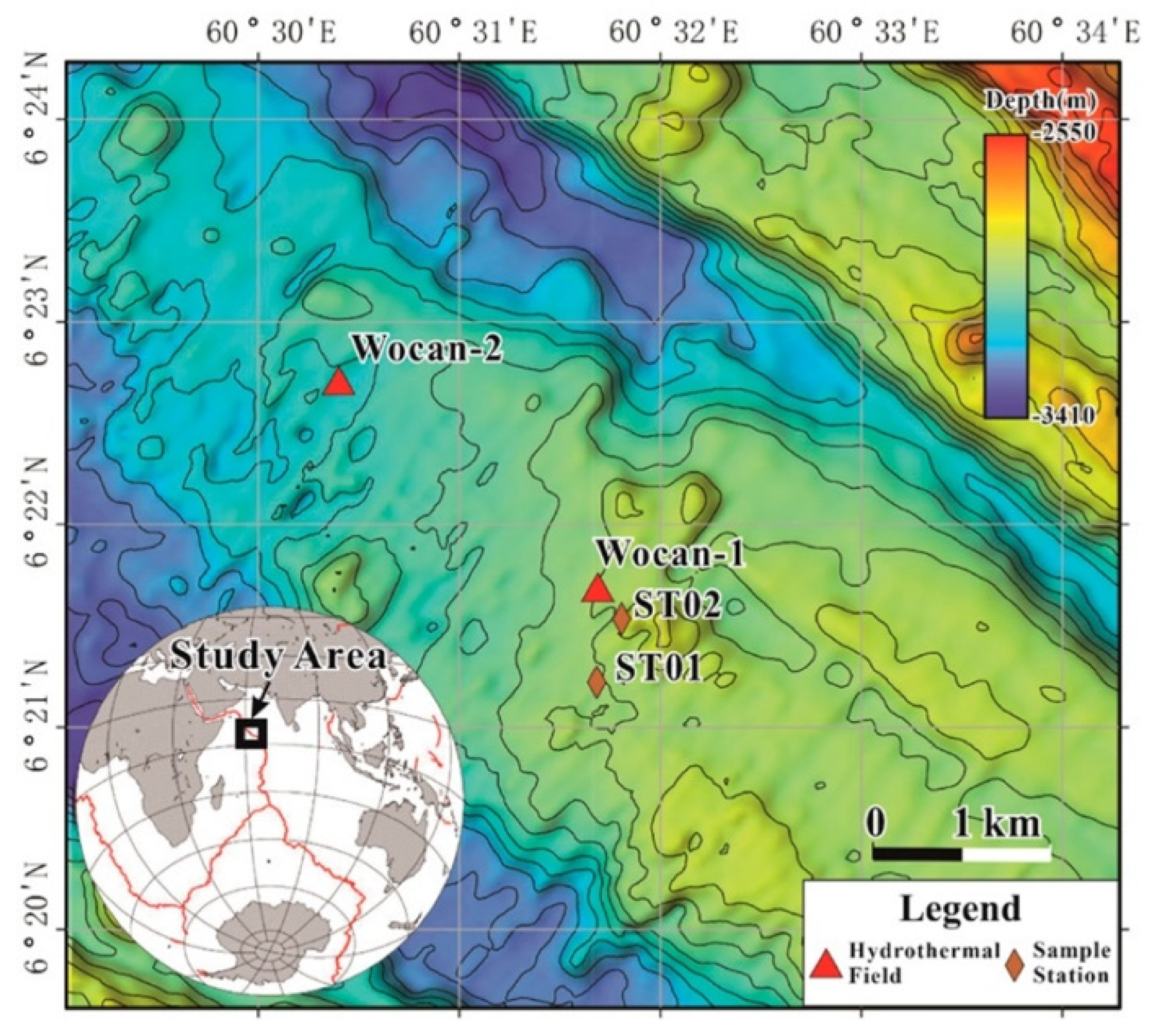
3.1. Grid Configuration and Boundary Conditions

As depicted in Figure 3, the computational domain for the reference case was primarily guided by Lowell [25] and Wang [19], with a depth of 1 km and longitudinal width of 2 km. On the model’s left, a hydrothermal recharge zone, measuring 600 m in width and 950 m in depth, was constructed. This aligns with findings from Lowell and Yao [26], suggesting that ridge crest hydrothermal recharge areas must be expansive to prevent blockage from anhydrite precipitation. We also postulate narrow cross-flow and discharge areas, each 50 m in width, to emulate discharge via high-permeability fault and fracture zones. An unstructured triangular grid was generated using Gmsh (version 3.0.0, https://gmsh.info/), with a grid size of approximately 7 m. For a 1000 m high model, the node count is 33,648 and the grid count is 65,080. In the numerical model, a constant porosity is assumed throughout the finite element mesh. This simplification is adopted to facilitate the computational process while maintaining a reasonable degree of accuracy in our simulations. It should be noted that this uniform porosity assumption applies to the entire model domain, as depicted in Figure 3. Porosity may vary with depth and other geological factors. However, for the purpose of this study, where the focus is on a broader understanding of hydrothermal fluid dynamics, a constant porosity is deemed an acceptable approximation.

The system’s upper region is overlaid with seawater, maintaining a consistent pressure of 30 MPa. This pressure linearly accumulates with depth, starting from an initial 30 MPa at the top (corresponding to an oceanic depth of 3000 m) to 40 MPa at the bottom. The computational domain’s upper boundary interfaces with the oceanic fluid, utilizing mixed-temperature boundary conditions: the zero-gradient boundary condition is applied for positive velocities, while the fixed-value boundary condition is employed for negative (downward) velocities. A fixed-value pressure boundary condition is used, set at 30 MPa for this scenario. The lower boundary, representing the deep oceanic crust, uses a fixed non-uniform temperature boundary condition, with temperatures linearly increasing from left to right, unaffected by time. A zero-flux boundary condition, typical for adiabatic impermeable boundaries, is applied for pressure. Both the left and right boundaries, distant from the channels’ crust boundaries, utilize zero-gradient temperature and zero-flux pressure boundary conditions. Given the addition of ion concentration computations, initial and boundary conditions for ion concentrations are set. The initial ion concentration within the computational domain is assumed to be the seawater element concentration (set to 0 mmol/kg). Boundary conditions for element concentration mirror those for temperature, with the upper boundary adopting a mixed condition, allowing element inflow and outflow. The bottom boundary applies a fixed-value boundary condition with a given element concentration C_boundary, while the left and right boundaries use the zero-flux boundary condition.

3.2. Model Parameter Settings

In 2022, Chen et al [27] based on graphical regional inter-relationship algorithms, analyzed the data of the Wocan-1 hydrothermal field in the north-west Indian Ocean, and estimated that the heat input into the ocean by the “Flaming Hill” in the north-west Indian Ocean was about 1.35 ± 0.11 MW, and the Fe flow volume was about 3661 ± 323 kg/year. Based on the above heat flow estimate and Fe flow estimates, it is possible to construct a two-dimensional numerical model of the heat fluid cycle of WHF-1, and use HydrothermalFoam to simulate the hydrothermal fluid circulation process in the ocean shell as well as the element transfer process in hydrothermal fluid. A single-pass model is employed for the simulation, a model frequently used for estimating certain characteristics of hydrothermal fields, such as the material flow rate Q and permeability k of the heat recharge zone [9,28]. Given the known heat flux (H) at the hydrothermal vent, the fluid temperature (Td) at the vent, and the estimated area of the vent region (A_d = 400 m²), Equations (7) and (8) can be utilized to estimate the flow rate at the vent and the permeability of the hydrothermal discharge area. The simulation results are then combined with actual data from the vent to invert the initial conditions and constrain the model parameters.

$$Q=\frac{H}{c_{ht}{T}_d}$$

(7)

$$k_d=\frac{Q{\nu }_d}{{\rho }_{f0}{a}_{d}g{T}_d{A}_d}$$

(8)

where $c_{ht}$ ≈ 5 × 10³ J kg⁻¹, ${\nu }_d$ ≈ 10–7 m² s⁻¹, and $a_d$ ≈ 10⁻³ °C⁻¹, represent the specific heat capacity, kinematic viscosity, and coefficient of thermal expansion of the fluid at the hydrothermal vent, respectively [9]; ${\rho }_{f0}$ = 1000 kg m⁻³ denotes the density of the fluid at 0 °C; $g$ = 9.8 m s⁻² is the gravity acceleration; $A_d$ = 400 m² is the estimated hydrothermal vent area—it is worth noting that the calculations of the subsequent examples are based on this assumption, which can be modified later after obtaining more accurate data; $T_d$ = 359 °C, which is the fluid temperature at the vent [17]; $H$ = 1.35 ± 0.11 MW denotes the heat flux from the hydrothermal vent [27]. Substituting the above parameters into Equations (7) and (8), the flux at the vent $Q$ = 0.75 ± 0.06 kg s⁻¹ and the permeability of the hydrothermal recharge zone $k_d$ = 5.3 ± 0.4 × 10⁻¹⁴ m² can be obtained.

Chen et al. [27] estimated that the Fe flux to the ocean from the hydrothermal vent of WHF-1 was about 3661 ± 323 kg/a, from which the mass of elements released into the ocean from the hydrothermal vents of WHF-1 can be estimated by Equation (9) [29].

$$C=\frac{m}{Q\rho M}$$

(9)

where $C$ is the element concentration; $M$ is the molar mass (the molar mass of Fe is 56 g/mol); $\rho$ is the density of the hydrothermal fluid, which is taken as 0.8 kg/m³ [30]; and $m$ is the mass of the element released into the ocean by the hydrothermal vent, which is taken as 3661 ± 323 kg/year. It can be estimated that the concentration of Fe in the “Flaming Hill” vents fluid in the WHF-1, $C_{\mathrm{vent}}$, is 2.59 ± 0.03 mmol/kg. The values and meanings of key parameters in the model can be found in

Table 1. Values of model key parameters.

Notation	Meaning	Value	Unit	Remarks
Td	Vent temperature	359	°C	Wang et al., 2017 [16]
H	Vent heat flux	1.35 ± 0.11	MW	Chen et al., 2022 [27]
Ad	Vent area	400	m2	Assumption
Q	Flux	0.75 ± 0.06	kg/s	Derived from Equation (7)
kd	Oceanic crust permeability	5.3 × 10−14	m2	Derived from Equation (8)
Cvent	Concentration of Fe at vent	2.59 ± 0.03	mmol/kg	Derived from Equation (9)
Cboundary	Concentration of Fe at bottom	/	mmol/kg	Sensitivity analysis
h	Depth of heat source	/	m	Sensitivity analysis
Tmax	Maximum temperature at heat source	/	°C	Sensitivity analysis

A_d = 400 m² is the estimated hydrothermal vent area; it is worth noting that the calculations of the subsequent examples are based on this assumption, which can be modified later after obtaining more accurate data.

.

3.3. Numerical Simulation Conditions

We set up a series of working conditions with different bottom temperature conditions through the simulation to reach the calculated steady state after obtaining the fluid temperature at the vent and the actual data at the vent for comparison and verification, and we carried out a sensitivity analysis of the bottom temperature conditions. The conditions of a series of working conditions with different bottom temperatures are given in

Table 2. Conditions with different bottom temperatures (Case 1.2 is the base case.).

Cases	Heat Source Depth (h/m)	Permeability at Recharge Area (kd/m2)	Calculation Time (a)	Bottom Minimum Temperature (Tmin/°C)	Bottom Maximum Temperature (Tmax/°C)
1.1	1000	5.3 × 10−14	600	300	500
1.2	1000	5.3 × 10−14	600	350	550
1.3	1000	5.3 × 10−14	600	400	600
1.4	1000	5.3 × 10−14	600	450	650
1.5	1000	5.3 × 10−14	600	500	700

.

In addition to the heat source temperature condition, the heat source depth is also a very important variable affecting the vent fluid temperature in seafloor hydrothermal systems. The simulation conditions with different heat source depths h were set up to combine both temperature conditions and heat source depths to study the effects. The details are given in

Table 3. Conditions with combinations of different bottom temperatures and heat source depths.

Cases	Heat Source Depth (h/m)	Permeability at Recharge Area (kd/m2)	Calculation Time (a)	Bottom Maximum Temperature (Tmax/°C)
2.1~2.5	1000	5.3 × 10−14	600	500~700
3.1~3.5	500	5.3 × 10−14	600	500~700
4.1~4.5	1500	5.3 × 10−14	600	500~700
5.1~5.5	2000	5.3 × 10−14	600	500~700
6.1~6.5	2500	5.3 × 10−14	600	500~700

Cases 2.1~2.5 correspond to Tmax values ranging from 500 °C to 700 °C. Specifically, for Case 2.1, Tmax is 500 °C; for Case 2.2, Tmax is 550 °C; for Case 2.3, Tmax is 600 °C; for Case 2.4, Tmax is 650 °C; for Case 2.5, Tmax is 700 °C. Subsequent cases follow the same pattern. In addition, to strike a balance between computational stability and efficiency, the calculation domain of the working conditions calculated by this table is different from that of the base case. It is only used for sensitivity analysis of heat source temperature and heat source depth. While qualitative conclusions can be derived, the quantitative results should be taken as references only.

for the setup of simulation conditions with different heat source temperatures and different heat source depths. The simulation conditions for different heat source temperatures at the same heat source depth were set as a group, similar to the case in Table 2. For example, simulation conditions 2.1–2.5 represent the case where the heat source temperature is 500 m and the heat source temperature increases from 500 °C to 700 °C in 50 °C increments.

Taking the element Fe as an example, to calculate the element concentration we set up a series of simulation conditions with different bottom Fe concentrations. After the numerical simulation reached the computational steady state, we carried out the verification of the Fe elemental concentration of the fluid at the vent in comparison with the actual data at the vent, which could be used to carry out the sensitivity analysis of the conditions of the bottom element concentration, and a series of simulation conditions with different bottom temperatures are given in

Table 4. Conditions with different bottom Fe element concentrations.

Cases	Heat Source Depth (h/m)	Permeability at Recharge Area (kd/m2)	Calculation Time (a)	Bottom Fe Element Concentration (Cboundary /mmol·kg−1)
7.1	1000	5.3 × 10−14	600	5
7.2	1000	5.3 × 10−14	600	10
7.3	1000	5.3 × 10−14	600	15
7.4	1000	5.3 × 10−14	600	20

In this paper, the concentration calculations and analyses of elements are exemplified using Fe (iron). Unless specified otherwise, all subsequent discussions and analyses concerning elemental concentration pertain to Fe.

for the model setting. We primarily focused on iron (Fe) as an example to demonstrate our approach. However, the same methodology can be applied to other elements as well. By modifying the molar mass in Equation (9) and utilizing the concentrations observed at the vent sites, it is certainly possible to estimate the concentrations of other elements like Zn, Ag, and Au.

4. Results and Discussion

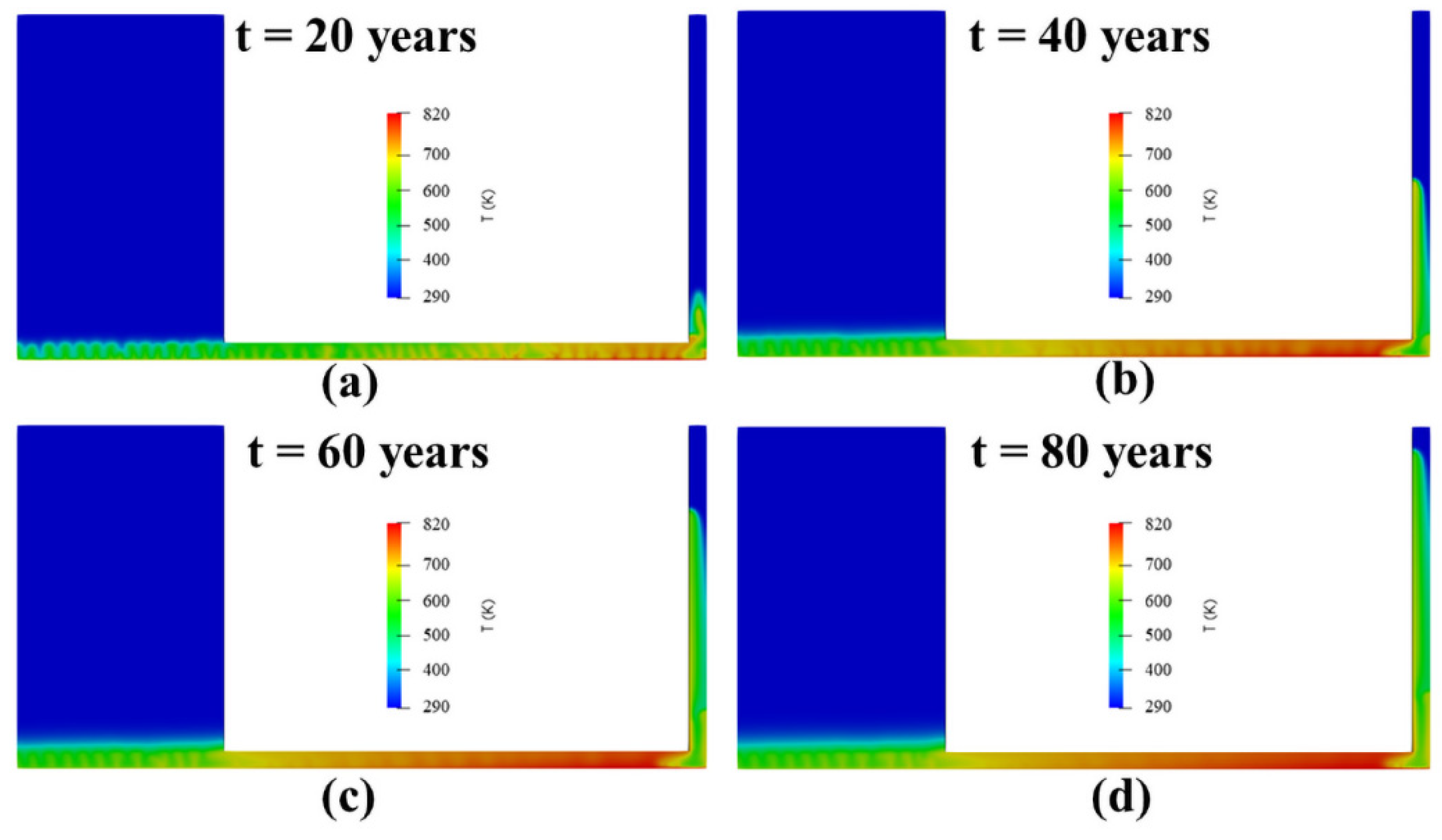
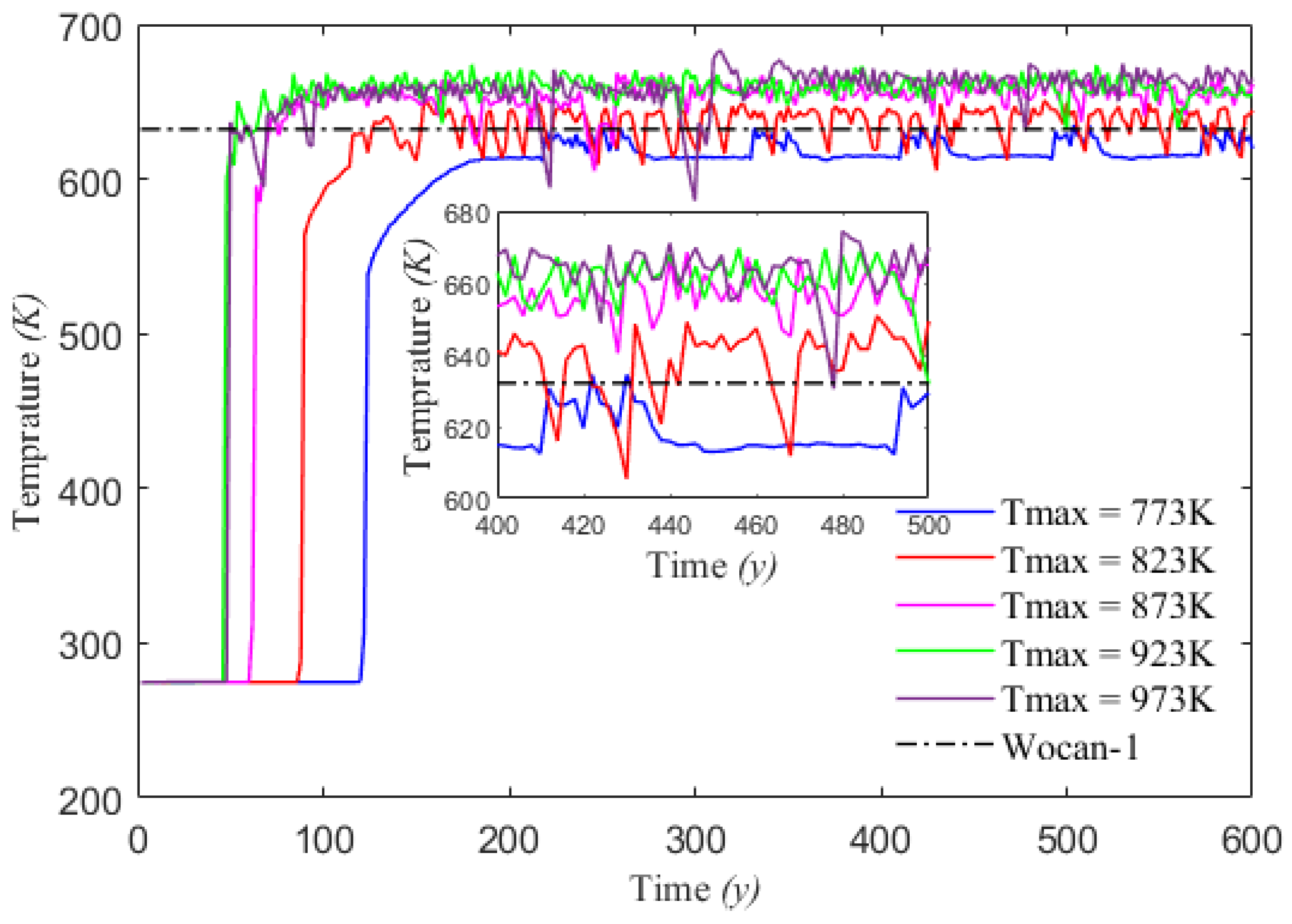
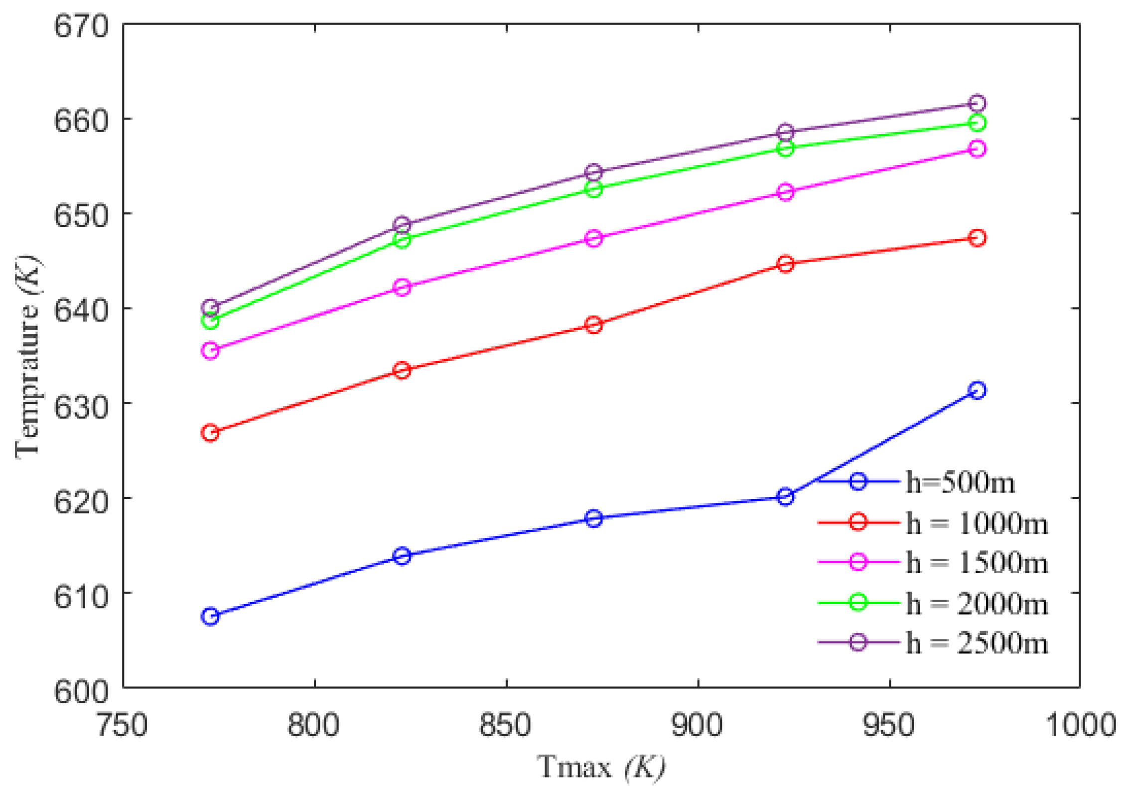
4.1. Hydrothermal Fluid Temperature and Its Influencing Factors

Using Case 1.2 as the base case (refer to Table 2), we studied the temperature variations in the hydrothermal fluid under this condition (as shown in Figure 4) and selected four typical moments where temperature changes were particularly pronounced. As the calculation time increases, the fluid temperature in the middle channel of the left and right branches first increases and then remains basically stable. As the hydrothermal fluid rises up, the temperature of the left branch also gradually rises. It can be seen from Figure 4a,d that during the simulation time from 20 years to 80 years, the high-temperature hydrothermal fluid has been rising but has not reached the seabed. The right branch belongs to the hydrothermal recharge area, and the temperature change is not obvious.

Figure 5 presents the temporal temperature variations in fluid at the vent for Cases 1.1–1.5. Within the figure, lines of distinct colors signify varying maximum temperatures at the bottom, increasing from 773K (500 °C) to 973K (700 °C). The black dotted line denotes the fluid temperature of the hydrothermal vent for the “Flaming Hill” in the WHF-1. It can be seen from the figure that the time required for hydrothermal fluid to reach the seafloor is different under different heat source temperatures. The higher the temperature, the quicker it reaches the seafloor. Under the calculation conditions given in this article, under the condition of Tmax = 773K, it takes ~130 years for the hydrothermal fluid to reach the seafloor, and under the condition of Tmax = 823K, it only takes ~80 years for the hydrothermal fluid to reach the seafloor. In addition, it can be seen from Figure 5 that after the hydrothermal fluid reaches the seafloor, the temperature of the fluid at the vent fluctuates within a certain range, but remains stable overall. For the base case (Case 1.2), the average temperature at the vent during the period from 200 to 600 years stands at 636K (approximately 363 °C). With certain fluctuations over time, this temperature can be up to a maximum of 647K (approximately 374 °C), and the lowest can be reduced to 613K (about 340 °C). By partially magnifying the temperature changes during the period from 400 to 500 years, it can be found that the actual temperature at the “Flaming Hill” hydrothermal vent of Wocan-1 closely aligns with the stabilized vent temperature when the bottom’s maximum temperature is set at 823K (550 °C).

The temperatures at which the vent reaches a steady state under the conditions outlined in Table 3 can be found in Figure 6. As shown in the figure, lines of different colors represent different heat source depths ranging from h = 500 m to h = 2500 m, and points on the same line from left to right represent working conditions where the heat source temperature gradually increases. To strike a balance between computational stability and efficiency, the calculation domain of the working conditions is different from that of the base case. It is only used for the sensitivity analysis of heat source temperature and heat source depth. While qualitative conclusions can be derived, the quantitative results should be taken as references only. It can be found that at the same heat source depth, as the heat source temperature increases, the temperature of the fluid at the vent continues to increase. Comparing this under the conditions of the same heat source temperature, it is not difficult to see that when the driving heat source of the hydrothermal circulation is shallow, the temperature of the hydrothermal vent increases as the depth of the heat source increases. The most significant increase in temperature occurs between depths of h = 500 m and h = 1000 m, while the lowest increase is noted between h = 2000 m and h = 2500 m. This conclusion seems to be different from what we expected, because as the depth of the heat source increases (i.e., the model depth h here), the fluid experiences a longer path during its rise, and thus the more heat is lost due to diffusion and expansion; so, the greater the depth of the heat source, the lower the temperature of the vent should be. However, as the depth of the system increases, so does the pressure, resulting in higher temperatures in the upwelling while also providing greater initial energy to compensate for the heat loss during fluid discharge. As Jupp et al. [31] pointed out, the upwelling temperature is consistent with the overall output power maximization trend, meaning it increases with the increase in pressure.

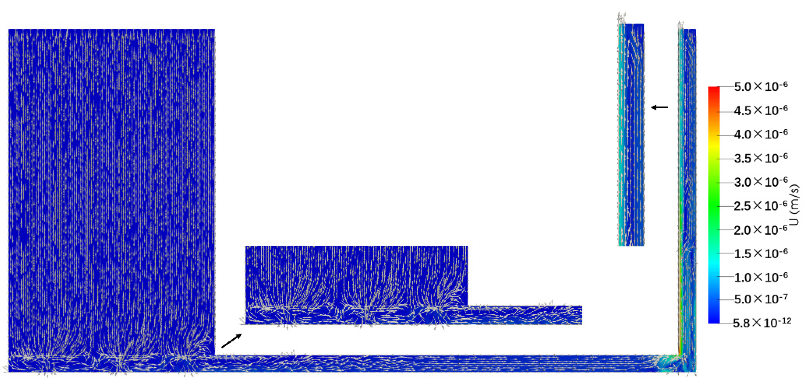
4.2. Velocity Field of Hydrothermal Fluid

We calculated the base case at 600 years and analyzed the hydrothermal fluid velocity field at that time (shown in Figure 7). As can be seen from the figure, the fluid in the left area is dominated by inflow, with a flow rate of approximately 3.15 × 10⁻⁹ m/s. The fluid forms an obvious vortex structure when entering the middle channel. The right branch part has both inflow and outflow, with the outflow being the main one. The flow rate of the outflow part can reach 1.5 × 10⁻⁶ m/s, and the flow speed of the inflow part is slightly smaller, about 1.5 × 10⁻⁷ m/s, which is about 10 times smaller than the outflow part. In the calculation area, the maximum flow velocity reaches 5 × 10⁻⁶ m/s, located at the bottom of the right branch. Due to the difference in permeability and temperature between the left and right branches, the flow velocity of the right branch is significantly greater than that of the left branch.

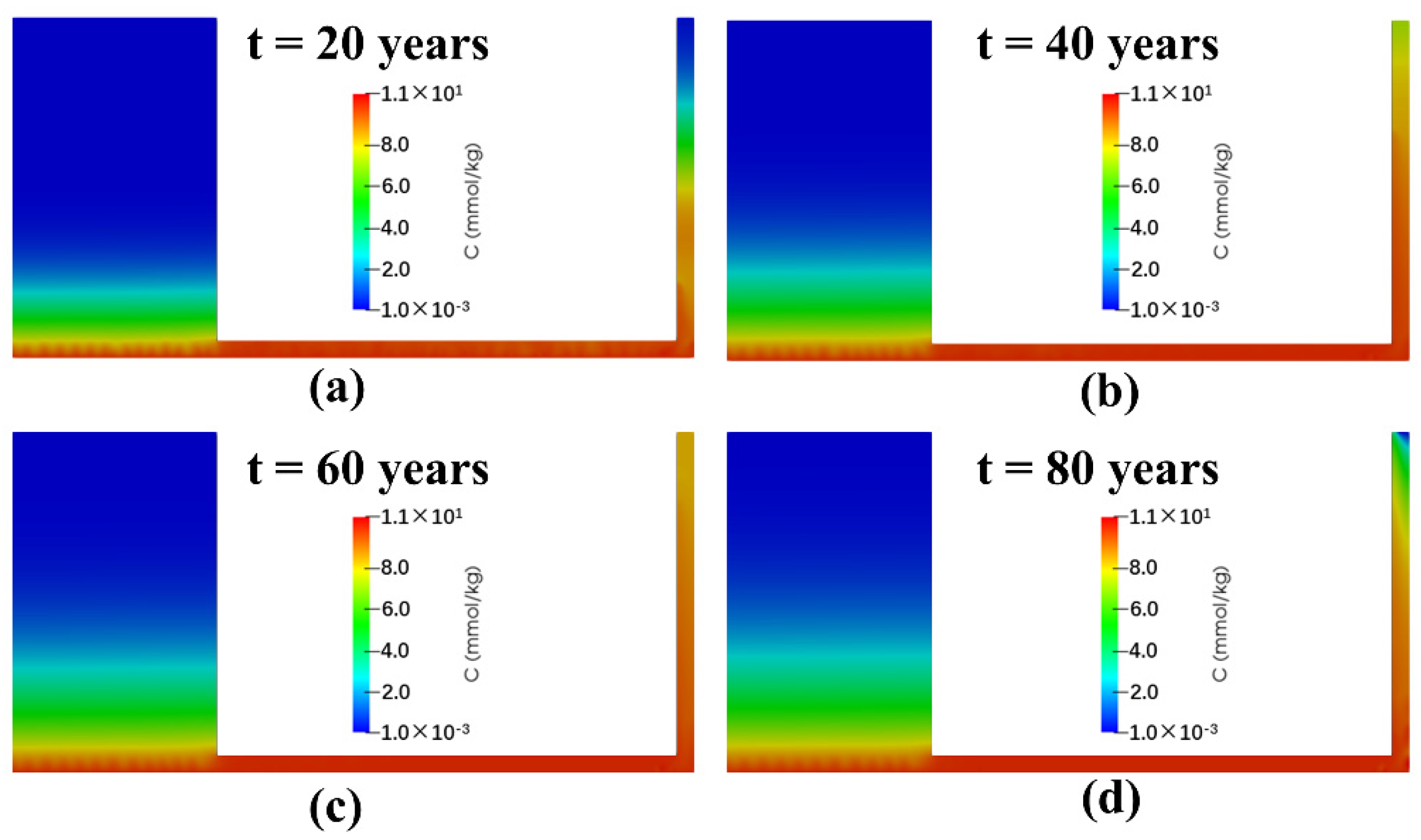
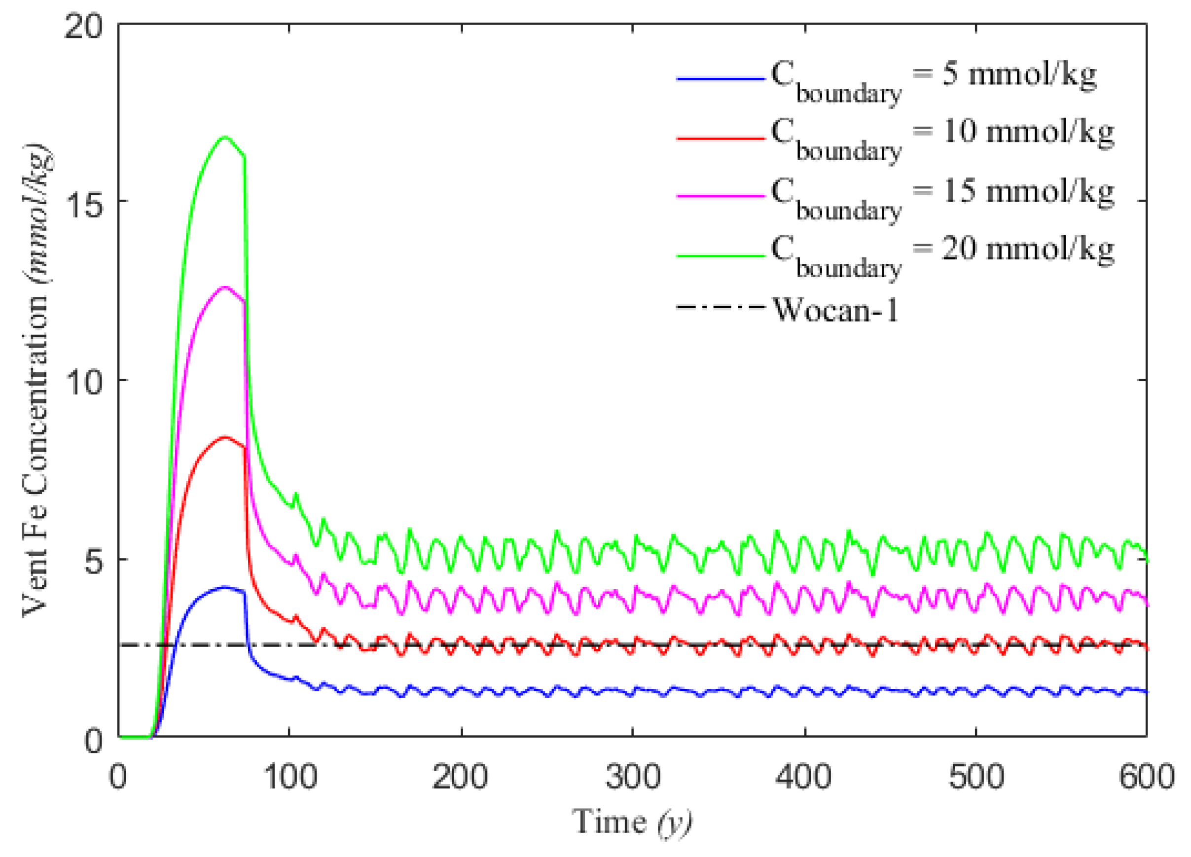
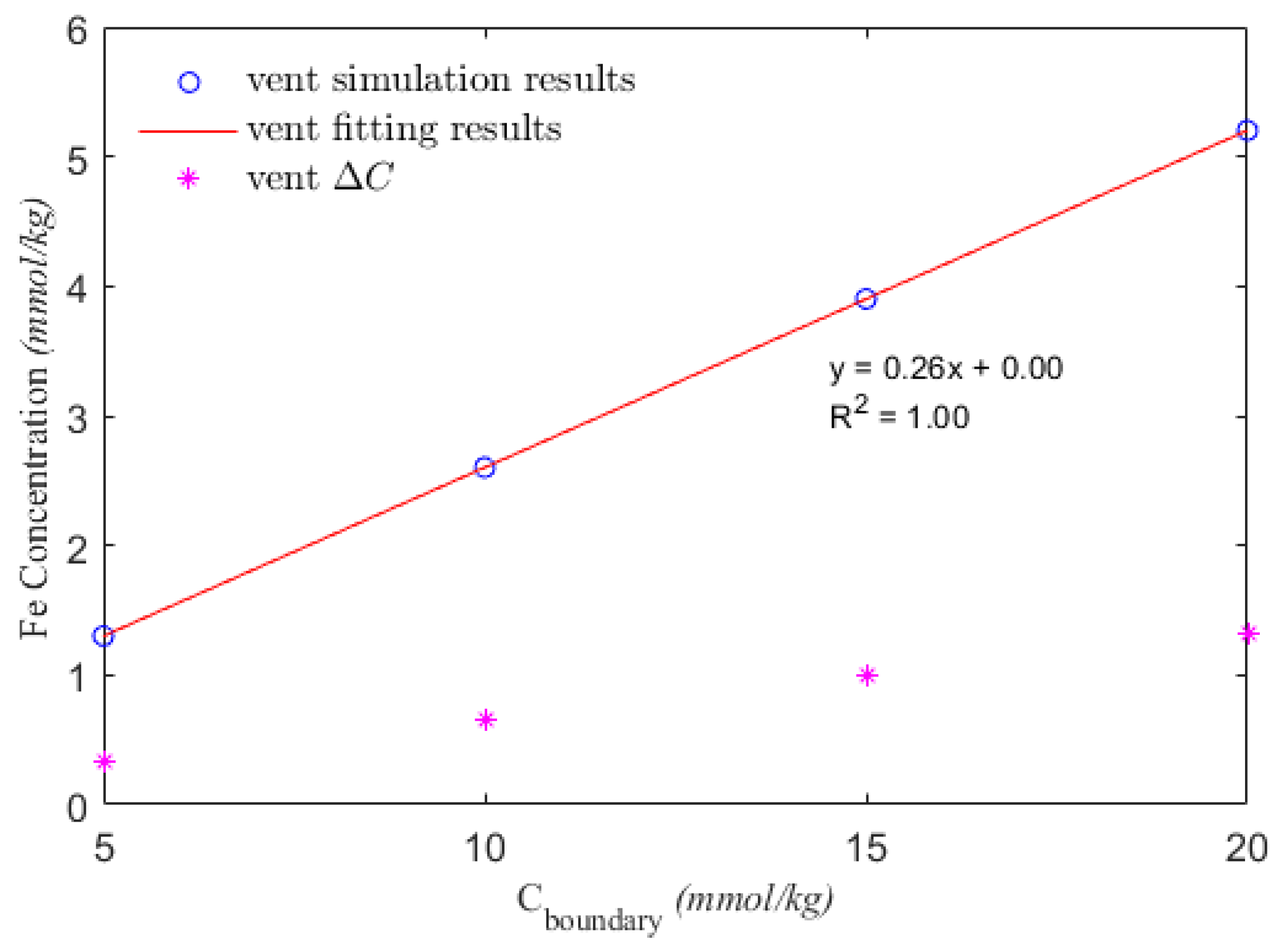
4.3. Relationship between Element Concentration at the Vent and the Concentration at the Bottom

The distribution of element concentrations at different times under the research condition (Case 1.2) is investigated, as depicted in Figure 8. The cycling of elements primarily takes into account convection and diffusion. The concentration in the left branch hydrothermal recharge zone is relatively low. Meanwhile, the concentration in the right branch hydrothermal discharge zone first increases (as shown in Figure 8a–c), followed by a noticeable decrease at the vent (Figure 8d). Combined with the flow field results in Figure 7, the reasons for the concentration reduction at the vent can be analyzed. On one hand, when the hydrothermal fluid reaches the seafloor, some elements are either carried away by the fluid or react with cold seawater, forming mineral precipitates near the vent. On the other hand, low-concentration fluids also flow into the vent, mixing and diluting with the high-concentration fluids.

Figure 9 displays the variation in concentration over time at the vent under four boundary conditions at the bottom: 5 mmol/kg, 10 mmol/kg, 15 mmol/kg, and 20 mmol/kg. The value represented by the black dashed line is the iron element concentration of the fluid at the vent in the WHF-1, calculated using Equation (9), with C_vent being 2.59 ± 0.03 mmol/kg. For all four conditions, after a period of simulation, a relatively stable state is reached with some degree of fluctuation. The average results from 200 to 600 years are taken as the simulated results in Figure 10. Based on these results, an empirical relationship can be derived: C_vent = 0.26 C_boundary. Moreover, the magnitude of concentration fluctuations during the period of 200 to 600 years was also analyzed, as depicted in Figure 10. It can be observed that the concentration fluctuation ($\mathsf{\Delta }C$) at the vent increases with the increase in bottom concentration. Given that the hydrothermal fluids currently obtainable are almost exclusively from the vent areas, it is challenging to acquire fluids from the deeper parts of the hydrothermal system. As a result, the bottom element concentration boundary conditions within the system can only be estimated and are difficult to validate against actual data.

5. Conclusions

• This paper constructs a numerical model for the hydrothermal region of the Carlsberg Ridge Worm-1 in the Indian Ocean. This model successfully reproduces the typical hydrothermal circulation processes of oceanic crust, yielding data on temperature distribution, flow field structure, and elemental concentration distribution. After simulating for a certain period, the depth and temperature of potential heat sources in the Worm-1 hydrothermal region are inferred based on the vent data. The maximum temperature of the heat source Tmax = 823K (550 °C) and the depth of the heat source h = 1 km are possible results. The model can be further refined with more field data in the future, making the results more targeted.
• A sensitivity analysis was carried out on the temperature and depth of the heat source. This analysis highlighted their pronounced effects on the fluid temperature at the vent. Specifically, within a certain range, the temperature of the heat source positively correlates with the fluid temperature at the vent. Similarly, the depth of the heat source also shows a positive correlation with the fluid temperature at the vent.
• In this study, we initially addressed the kinetic processes of elemental transport within hydrothermal circulation. While neglecting the impacts of chemical reactions among elements and microbial influences on the transport, an empirical relationship was formulated between the elemental concentration at the bottom boundary and the fluid elemental concentration at the vent: C_vent = 0.26 C_boundary. Future research can incorporate the effects of chemical reactions and microbial influences on elemental transport and related work will be carried out in the next step.

In summary, this paper establishes a numerical model for deep-sea hydrothermal fluid circulation based on the modified HydrothermalFoam. The model is applied to study the Worm-1 hydrothermal region of the Carlsberg Ridge in the Indian Ocean, enriching the existing numerical models of hydrothermal vents. The temperature distribution and elemental transport characteristics obtained from this research provide a basis for further exploration and utilization of the Wocan-1 hydrothermal field. Additionally, this model holds potential for application in the exploration of hydrothermal sulfide resources in other regions.

References

1. Hasenclever, J.; Theissen-Krah, S.; Rüpke, L.H.; Morgan, J.P.; Iyer, K.; Petersen, S.; Devey, C.W. Hybrid Shallow On-Axis and Deep off-Axis Hydrothermal Circulation at Fast-Spreading Ridges. Nature 2014, 508, 508–512. [Google Scholar] [CrossRef]
2. Elderfield, H.; Schultz, A. Mid-Ocean Ridge Hydrothermal Fluxes and the Chemical Composition of the Ocean. Annu. Rev. Earth Planet. Sci. 1996, 24, 191–224. [Google Scholar] [CrossRef]
3. Hodgkinson, M.R.S.; Webber, A.P.; Roberts, S.; Mills, R.A.; Connelly, D.P.; Murton, B.J. Talc-Dominated Seafloor Deposits Reveal a New Class of Hydrothermal System. Nat. Commun. 2015, 6, 10150. [Google Scholar] [CrossRef]
4. Jiang, Z.; Han, X.; Wang, Y. Characteristics of water chemistry and constituents of particles in the hydrothermal plume near 6° 48′ N, Carlsberg Ridge, Northwest Indian Ocean. J. Mar. Sci. 2017, 35, 34–43. (In Chinese) [Google Scholar]
5. Olatunde Popoola, S.; Han, X.; Wang, Y.; Qiu, Z.; Ye, Y. Geochemical Investigations of Fe-Si-Mn Oxyhydroxides Deposits in Wocan Hydrothermal Field on the Slow-Spreading Carlsberg Ridge, Indian Ocean: Constraints on Their Types and Origin. Minerals 2018, 9, 19. [Google Scholar] [CrossRef]
6. Qiu, Z.; Han, X.; Wang, Y.; Chen, X.; Garbe-Schönberg, D.; Fan, W.; Li, H.; Liu, J. Time-Series Records of Particulate Fluxes Reveal Temporal Variations in Hydrothermal Activity in the Wocan Hydrothermal Field, Carlsberg Ridge. Mar. Geol. 2023, 460, 107056. [Google Scholar] [CrossRef]
7. Weis, P.; Driesner, T.; Coumou, D.; Geiger, S. Hydrothermal, Multiphase Convection of H2O-NaCl Fluids from Ambient to Magmatic Temperatures: A New Numerical Scheme and Benchmarks for Code Comparison. Geofluids 2014, 14, 347–371. [Google Scholar] [CrossRef]
8. Ingebritsen, S.E.; Geiger, S.; Hurwitz, S.; Driesner, T. Numerical Simulation of Magmatic Hydrothermal Systems. Rev. Geophys. 2010, 48, RG1002. [Google Scholar] [CrossRef]
9. Tao, C.; Seyfried, W.E.; Lowell, R.P.; Liu, Y.; Liang, J.; Guo, Z.; Ding, K.; Zhang, H.; Liu, J.; Qiu, L.; et al. Deep High-Temperature Hydrothermal Circulation in a Detachment Faulting System on the Ultra-Slow Spreading Ridge. Nat. Commun. 2020, 11, 1300. [Google Scholar] [CrossRef]
10. He, Z.; Han, X.; Qiu, Z.; Wang, Y.; Lou, Y. Numerical modeling of hydrodynamic processes of deep-sea hydrothermal plumes: A case study on Daxi hydrothermal field, Carlsberg Ridge. Sci. Sin.-Technol. 2020, 50, 194–208. [Google Scholar] [CrossRef]
11. Yapparova, A.; Gabellone, T.; Whitaker, F.; Kulik, D.A.; Matthäi, S.K. Reactive Transport Modelling of Dolomitisation Using the New CSMP++GEM Coupled Code: Governing Equations, Solution Method and Benchmarking Results. Transp. Porous Med. 2017, 117, 385–413. [Google Scholar] [CrossRef]
12. Theissen-Krah, S.; Iyer, K.; Rüpke, L.H.; Morgan, J.P. Coupled Mechanical and Hydrothermal Modeling of Crustal Accretion at Intermediate to Fast Spreading Ridges. Earth Planet. Sci. Lett. 2011, 311, 275–286. [Google Scholar] [CrossRef]
13. Pierre, S.; Gysi, A.P.; Monecke, T. Fluid Chemistry of Mid-Ocean Ridge Hydrothermal Vents: A Comparison between Numerical Modeling and Vent Geochemical Data. Geofluids 2018, 2018, 1389379. [Google Scholar] [CrossRef]
14. Fan, Q.; Li, J. Study on the influence of the structure of oceanic crust permeability on the hydrothermal convection—Based on thermodynamic modelling. Chin. J. Geophys. 2020, 63, 1986–1997. (In Chinese) [Google Scholar]
15. Kamesh Raju, K.A.; Chaubey, A.K.; Amarnath, D.; Mudholkar, A. Morphotectonics of the Carlsberg Ridge between 62°20′ and 66°20′E, Northwest Indian Ocean. Mar. Geol. 2008, 252, 120–128. [Google Scholar] [CrossRef]
16. Tao, C.; Wu, G.; Deng, X.; Qiu, Z.; Han, C.; Long, Y. New discovery of seafloor hydrothermal activity on the Indian Ocean Carlsberg Ridge and Southern North Atlantic Ridge—Progress during the 26th Chinese COMRA cruise. Acta Oceanol. Sin. 2013, 32, 85–88. [Google Scholar] [CrossRef]
17. Wang, Y.; Han, X.; Petersen, S.; Frische, M.; Qiu, Z.; Li, H.; Li, H.; Wu, Z.; Cui, R. Mineralogy and Trace Element Geochemistry of Sulfide Minerals from the Wocan Hydrothermal Field on the Slow-Spreading Carlsberg Ridge, Indian Ocean. Ore Geol. Rev. 2017, 84, 1–19. [Google Scholar] [CrossRef]
18. Qiu, Z.; Han, X.; Li, M.; Wang, Y.; Chen, X.; Fan, W.; Zhou, Y.; Cui, R.; Wang, L. The Temporal Variability of Hydrothermal Activity of Wocan Hydrothermal Field, Carlsberg Ridge, Northwest Indian Ocean. Ore Geol. Rev. 2021, 132, 103999. [Google Scholar] [CrossRef]
19. Wang, K.; Han, X.; Wang, Y.; Cai, Y.; Qiu, Z.; Zheng, X. Numerical Simulation-Based Analysis of Seafloor Hydrothermal Plumes: A Case Study of the Wocan-1 Hydrothermal Field, Carlsberg Ridge, Northwest Indian Ocean. J. Mar. Sci. Eng. 2023, 11, 1070. [Google Scholar] [CrossRef]
20. Sander, S.G.; Koschinsky, A. Metal Flux from Hydrothermal Vents Increased by Organic Complexation. Nat. Geosci. 2011, 4, 145–150. [Google Scholar] [CrossRef]
21. Xie, Q.; Han, X.; Wei, M.; Qiu, Z.; Dong, C.; Wu, Y.; Wu, X.; Yu, J. Characteristics and evolution of bacterial communities in the Wocan hydrothermal plume-influenced zone, Carlsberg Ridge, northwestern Indian Ocean. Acta Microbiol. Sin. 2022, 62, 1974–1985. (In Chinese) [Google Scholar] [CrossRef]
22. Wei, M.; Zeng, X.; Han, X.; Shao, Z.; Xie, Q.; Dong, C.; Wang, Y.; Qiu, Z. Potential Autotrophic Carbon-Fixer and Fe(II)-Oxidizer Alcanivorax Sp. MM125-6 Isolated from Wocan Hydrothermal Field. Front. Microbiol. 2022, 13, 930601. [Google Scholar] [CrossRef] [PubMed]
23. Li, J.; Mara, P.; Schubotz, F.; Sylvan, J.B.; Burgaud, G.; Klein, F.; Beaudoin, D.; Wee, S.Y.; Dick, H.J.B.; Lott, S.; et al. Recycling and Metabolic Flexibility Dictate Life in the Lower Oceanic Crust. Nature 2020, 579, 250–255. [Google Scholar] [CrossRef] [PubMed]
24. Guo, Z.; Rüpke, L.; Tao, C. HydrothermalFoam v1.0: A 3-D Hydrothermal Transport Model for Natural Submarine Hydrothermal Systems. Geosci. Model. Dev. 2020, 13, 6547–6565. [Google Scholar] [CrossRef]
25. Lowell, R.P.; Gosnell, S.; Yang, Y. Numerical Simulations of Single-pass Hydrothermal Convection at Mid-Ocean Ridges: Effects of the Extrusive Layer and Temperature-dependent Permeability. Geochem. Geophys. Geosyst. 2007, 8, Q10011. [Google Scholar] [CrossRef]
26. Lowell, R.P.; Yao, Y. Anhydrite Precipitation and the Extent of Hydrothermal Recharge Zones at Ocean Ridge Crests. J. Geophys. Res. 2002, 107, 2183. [Google Scholar] [CrossRef]
27. Chen, Y.; Lou, Y.; He, Z.; Wang, Y.; Qiu, Z.; Han, X. Flow fields and outputs of the hydrothermal plume at the Wocan-1 field based on an in-situ video. Sci. Sin.-Technol. 2022, 52, 1705–1715. [Google Scholar] [CrossRef]
28. Lowell, R.P.; Farough, A.; Hoover, J.; Cummings, K. Characteristics of Magma-driven Hydrothermal Systems at Oceanic Spreading Centers. Geochem. Geophys. Geosyst. 2013, 14, 1756–1770. [Google Scholar] [CrossRef]
29. Baker, E.T.; Massoth, G.J. Characteristics of Hydrothermal Plumes from Two Vent Fields on the Juan de Fuca Ridge, Northeast Pacific Ocean. Earth Planet. Sci. Lett. 1987, 85, 59–73. [Google Scholar] [CrossRef]
30. Kretschmar, U.; McBride, D. The Metallogeny of Lode Gold Deposits: A Syngenetic Perspective; Elsevier: Amsterdam, The Netherlands, 2015; pp. 151–198. [Google Scholar] [CrossRef]
31. Jupp, T.E.; Schultz, A. Physical Balances in Subseafloor Hydrothermal Convection Cells. J. Geophys. Res. 2004, 109, B05101. [Google Scholar] [CrossRef]
Figure 1. Bathymetric map of the study area showing the locations of the Wocan−1 and Wocan−2 hydrothermal fields and the mooring stations for ocean current observation ST01 and ST02 (quote from Wang et al., 2023) [19].
Jmse 12 00046 g001
Figure 2. Calculation flow chart (modified from Guo et al., 2020) [24].
Jmse 12 00046 g002
Figure 3. Schematic of the grid for the reference case.
Jmse 12 00046 g003
Figure 4. Temperature field at different moments for Case 1.2. (a) Temperature field at t = 20 years; (b) Temperature field at t = 40 years; (c) Temperature field at t = 60 years; (d) Temperature field at t = 80 years.
Jmse 12 00046 g004
Figure 5. Temporal variation in fluid temperature at the vent for Cases 1.1–1.5.
Jmse 12 00046 g005
Figure 6. The fluid temperatures at the vent at a steady state under the conditions presented in Table 3.
Jmse 12 00046 g006
Figure 7. Velocity field diagram at 600 years for Case 1.2.
Jmse 12 00046 g007
Figure 8. Concentration field at different moments for Case 1.2. (a) Concentration field at t = 20 years; (b) Concentration field at t = 40 years; (c) Concentration field at t = 60 years; (d) Concentration field at t = 80 years.
Jmse 12 00046 g008
Figure 9. Temporal variation in Fe concentration at the vent for Cases 7.1–7.4.
Jmse 12 00046 g009
Figure 10. Simulation results of vent concentration (average from 200 to 600 years) and Δ C for Cases 7.1–7.5.
Jmse 12 00046 g010