Hydrodynamic Interactions between Ships in a Fleet

Abstract

There has always been a concern about the hydrodynamic interaction between ships in a flow field. In this study, the RANS method is utilized, and the hydrodynamic interference between two KRISO Container Ships (KCS) operating in still water with identical parameters and sailing at the same speed is investigated. Overlapping grids are used to simulate ship motion, and the VOF method is used to simulate the free surface. A KCS ship model of 1:1 size without propeller is used in the study. In order to study the change principle of the Kelvin flow field created by a single ship, the resistance coefficient and the flow field surrounding the ship are first calculated for the monohull case. Then the influence of interference between two ships is examined at various speeds and intervals and compared with the monohull case. It is discovered that the resistance coefficient of the following ship is reduced in a certain speed interval under the influence of the leading ship, where the maximum reduction can be up to 24.3%. The reason for this phenomenon may be that the wave around the following ship is superimposed on the transverse wave behind the leading ship. When the height of the wave is suppressed, the following ship’s resistance is reduced.

1. Introduction

Sea trains contain multiple hulls joined together to travel in formation. Sea trains utilize basic hydrodynamic principles that can reduce the resistance of a fleet of ships below the resistance of individual components traveling separately [1]. The principle of generation is related to wave interference generated by a single hull or multiple ships. When a ship is sailing in still water, it disturbs the surface of the water and produces a ship’s wake. This phenomenon is often referred to as a Kelvin wake. When a ship follows another ship, the Kelvin wake generated by the leading ship affects the following ship. So far, the characteristics of the waves generated by a monohull sailing in still water have been studied by many scholars. The wave of a ship sailing in still water is made up of transverse and divergent waves. Kelvin discovered that the wave generated by a ship sailing in still water lies within a wedge with an angle of 19°28′. Noblesse et al. [2] studied the wave interference between the bow and stern of a monohull using point source and point sink models located at the bow and stern, respectively. Zhang et al. [3] simulated the Kelvin flow of a monohull using a continuous distribution of sources and investigated that the apparent wake angle on the surface is very little affected by the shape of the hull. Transverse waves dominate when Fr < 0.6, and divergent waves dominate when Fr > 0.6. Darmon et al. [4] investigated the Kelvin wave characteristics at large Froude number and found that the angle of the wave impact area is the Kelvin angle, but the angle of the maximum amplitude of the wave is correlated with Fr-1 at large Froude number. Pethiyagoda et al. [5] also used a two-point model, complementing the case of small Froude number. For the same Fr, constructive interference or destructive interference occur in the transverse wave due to different intervals between the two points. Sun et al. [6] investigated the effects of ship speed and ship size on the waveform and showed that the wake angle decreases with increasing speed and increases with increasing ship size. In addition, for high ship speeds, the effect on wake angle may be more significant.

For the hydrodynamic interference between two or more objects side by side in the flow field, much research has also been carried out. Zhou et al. [7] summarized the hydrodynamic analysis of ship–ship interactions over the last decade. Zhou et al. [8] studied various hydrodynamic interaction problems between ships and other solid boundary objects including the seabed based on the potential flow model and the panel method, and carried out validation with experiments. Peng et al. [9] modeled the confinement effects in the maneuvering equations and investigated the maneuverability of ships at different spacing, speeds, and channel widths. Luo-Theilen et al. [10] proposed a motion model of mechanically coupled multi-body systems, which was utilized and validated in cases such as a floating tugboat. Wang et al. [11] predicted the hydrodynamic interference effects of two floating bodies in waves using three methods: 2D strip theory (STF), spectral analysis method, and time domain theory. Harada et al. [12] studied the resonance of two objects in a flow field by means of the potential flow method and the viscous flow method, respectively, and obtained the limits of environmental conditions for side-by-side offloading operations. Li et al. [13] used PIV flume tests, physical modeling tests of ship-bridge intersections, and numerical simulations to investigate the effect of different flow attack angles of round-end piers on moving ships, which focus on the moment and the ship’s motion attitude. Vasudevan et al. [14] investigated the hydrodynamic interaction forces between a ship in a moored condition and a passing ship by means of the CFD method, and the results show that the longitudinal and transverse forces on a moored ship are negligible when the spacing is greater than three times the width of the ship. Wnęk et al. [15] conducted a CFD study of the interaction forces on a small tugboat parallel to a large vessel in shallow water using various flow models and showed that the effect of viscosity was relatively weak in the calculations. Ekerhovd et al. [16] numerically investigated the resonant response of the fluid in the barge gap for three cases with different constraints when two barges are arranged side by side. Li et al. [17] focused on the gap resonance, and the hydrodynamic-associated wave elevation, added mass, wave force, etc., were analyzed in multi-body side-by-side configurations where the real hull shapes of FPSO and a ship are employed. Yuan et al. [18] found that the free surface must be considered even though the lateral separation between ships is large at high encountering speed. Li et al. [19] developed an iterative time-matching algorithm to solve the hydrodynamic interaction between high-speed ships considering the nonlinear free surface boundary condition in the time domain.

The case of ship fleets following each other fore and aft has also been studied by scholars. Yuan et al. [20] investigated the case of ducks swimming in a single line and found that in the region where destructive transverse wave interference occurs behind the lead duck, the wave resistance of the following ducks is reduced. Ma et al. [21] used a four-point model to consider the interference between the dominant waves created by the bow and the stern of the monohull as well as the interference between two ships, and investigated the characteristic of transverse wave and the wave resistance at medium and high Froude number. The relationship between the spacing between two ships and Fr which makes the resistance force of the following ship decrease is given.

There are currently fewer studies of two following ships, and it is unclear how two ships interact in cases similar to the ship fleet. In this study, numerical simulations are carried out for a single KRISO Container Ship (KCS) sailing in still water and two following ships, and the feasibility of the numerical method is validated by comparing with the experimental results. Overlapping grids are used to simulate ship motion, and the VOF method is used to simulate the free surface. A KCS ship model of 1:1 size without propeller is used in the study. The influence of the transverse wave generated by the leading ship on the resistance of the following ship and the characteristic of flow fields are analyzed under different Froude numbers and different intervals between the two ships, and the Froude number intervals that produce destructive interference are also analyzed. The numerical model is described in Section 2 of this paper. The simulation condition setting, verification and validation, and hydrodynamic interactions between two ships are presented in Section 3. Finally, Section 4 summarizes.

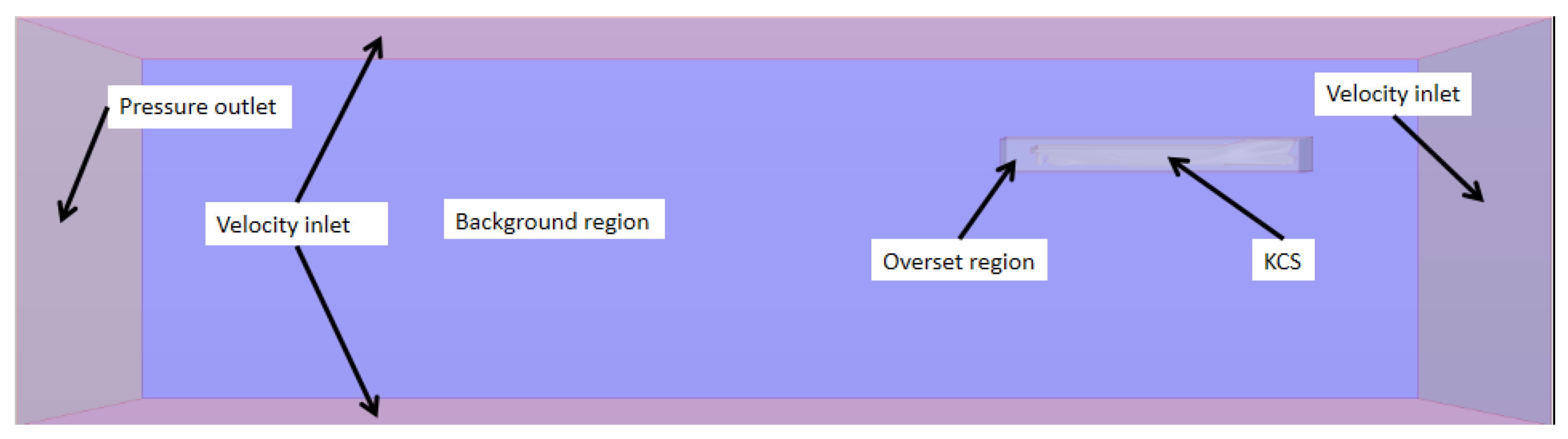
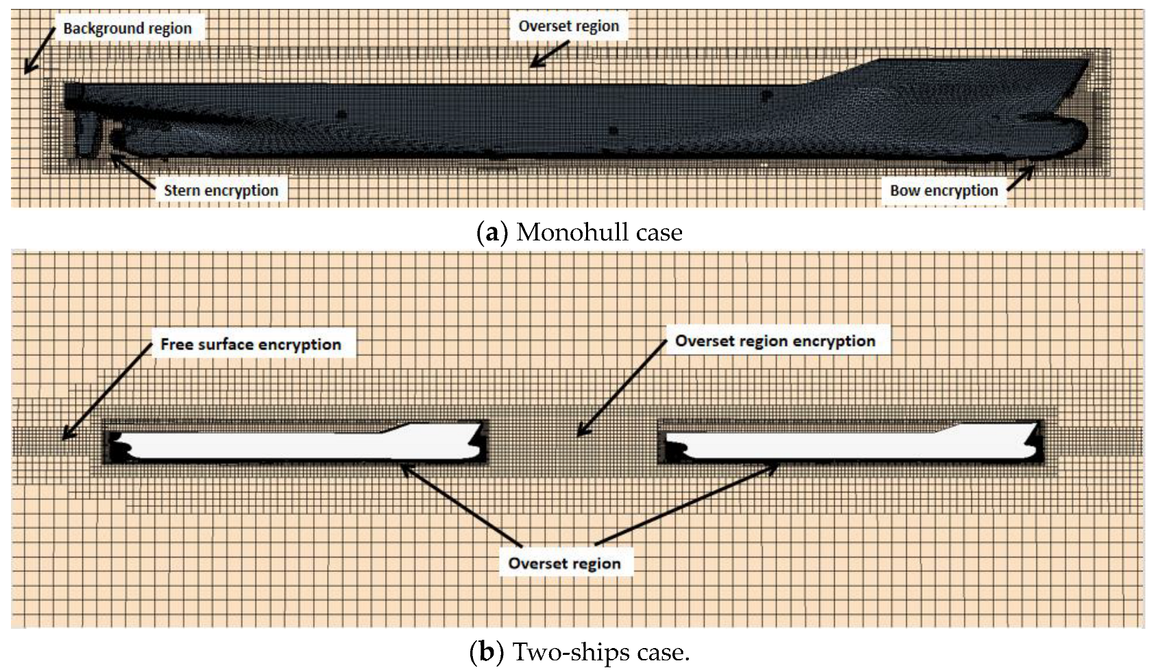
2. Numerical Modelling

In this study, commercial CFD software STAR-CCM+ is used. For incompressible flows without body forces, the averaged continuity and momentum equations can be written in tensor notation and Cartesian coordinates as [22]:

$$\frac{\partial \left(\rho {\overline{u}}_i\right)}{\partial x_i}=0$$

(1)

$$\frac{\partial \left(\rho {\overline{u}}_i\right)}{\partial t}+\frac{\partial }{\partial x_j}\left(\rho {\overline{u}}_i{\overline{u}}_j+\rho \overline{u_i^{’}{u}_j^{’}}\right)=-\frac{\partial \overline{p}}{\partial x_i}+\frac{\partial {\overline{\tau }}_{ij}}{\partial x_j}$$

(2)

$${\overline{\tau }}_{ij}=\mu \left(\frac{\partial {\overline{u}}_i}{\partial x_j}+\frac{\partial {\overline{u}}_j}{\partial x_i}\right).$$

(3)

where ${\overline{\tau }}_{ij}$ is the mean viscous stress tensor components, p is the mean pressure, ${\overline{u}}_i$ is the averaged Cartesian components of the velocity vector, $\rho \overline{u_i^{’}{u}_j^{’}}$ is the Reynolds stresses, $\rho$ is the fluid density, and $\mu$ is the dynamic viscosity.

To close the system of equations, a turbulence model needs to be introduced to express the Reynolds stress term in terms of known quantities. The turbulence model in this study based on the Boussinesq eddy-viscosity assumption, the expressions are defined [23]:

$$-\rho \overline{u_i^{’}{u}_j^{’}}=2{\mu }_t{\overline{\tau }}_{ij}-\frac{2}{3}\rho k{\delta }_{ij}$$

(4)

where ${\mu }_t$ is the eddy viscosity, ${\delta }_{ij}$ is the Kronecker-delta function, and $k$ is the turbulent kinetic energy.

Querard et al. [24] pointed out that the k-epsilon model can save 25% of CPU time over the k-omega model, So the k-epsilon model is chosen as a feasible option due to its economy. The closure equations for turbulence of k-epsilon model are [25]:

$$\rho \frac{\partial \left(u_{i}k\right)}{\partial x_i}=P_k+P_b-\rho \epsilon +\frac{\partial }{\partial x_i}\left[\left(\mu +\frac{{\mu }_t}{{\sigma }_k}\right)\frac{\partial k}{\partial x_i}\right]$$

(5)

$$\rho \frac{\partial \left(u_i\epsilon \right)}{\partial x_i}=\frac{\partial }{\partial x_i}\left[\left(\mu +\frac{{\mu }_t}{{\sigma }_e}\right)\frac{\partial \epsilon }{\partial x_i}\right]+C_1\frac{\epsilon }{k}\left(P_k+C_3{P}_b\right)-C_2\rho \frac{{\epsilon }^2}{k}$$

(6)

$${\mu }_t=\rho C_{\mu }\frac{k^2}{\epsilon }$$

(7)

$$P_{\kappa }={\mu }_t\left(\frac{\partial u_i}{\partial x_j}+\frac{\partial u_j}{\partial x_i}\right)\frac{\partial u_i}{\partial x_j}-\frac{\partial u_{\kappa }}{\partial x_{\kappa }}\left(3{\mu }_t\frac{\partial u_{\kappa }}{\partial x_{\kappa }}+\rho \kappa \right)$$

(8)

where P_k is the production of turbulent kinetic energy from the shear strain rate and is obtained from the time-averaged velocity field; P_b is the production of turbulent kinetic energy from buoyancy effects; ${\mu }_t$ is the turbulent viscosity; k is the turbulent kinetic energy; $\epsilon$ is the turbulent dissipation rate.

Although the standard model can handle boundary layer flows, overprediction of turbulent viscosity occurs in flow fields with large-scale separations or high mean shear rates, so the turbulent viscosity term is corrected in the realizable k-epsilon model to overcome the incorrect physical approach, and the dissipation term is corrected by adding a function [26].

The Volume of Fluid method (VOF) is used to track the free fluid surface [27]. It is an interface tracking method that is based on an Eulerian grid. In this method, different fluid components that are not compatible with each other share a set of momentum equations. The interface between the phases in the computational domain is tracked by using the phase volume fraction variable. When the volume fraction $\alpha$_k = 1, it means that water phase is present at that location. When $\alpha$_k = 0, it means that no water phase is present at that location. And when 0 < $\alpha$_k < 1, it means that the location is a sub-interface. The continuity equation of the VOF method is as follows:

$$\frac{\partial {\alpha }_k}{\partial t}+\frac{\partial }{\partial x_i}\left({\alpha }_k{u}_i\right)=0$$

(9)

In an overlapping grid, also called a nested grid, the core idea is to split the computational domain into multiple sub-grids with overlapping or nested relationships. Each set of sub-meshes is integrated into a set of processable whole meshes through transfer relations set on the overlapping boundaries. When an object moves within the flow field, the sub-grids containing the object move along with it and exchange flow field information through overlapping boundary difference transfer, thus realizing the simulation of the whole flow field. When using the overlapping mesh technique, the flow field needs to be pre-processed by removing redundant or invalid mesh nodes through digging holes and by establishing embedded mesh relationships to assemble the sub-mesh. The advantage of the overlapping mesh technique is that it reduces the difficulty of mesh generation, and at the same time, it can release the constraints of objects on the background mesh. Therefore, it can realize that the object can move freely in the flow field, and it can better solve for the case of large displacement of the object. Therefore, it is widely used in solving the problems of ship motion response in marine engineering.

3. Numerical Calculations and Results Analysis

3.1. Simulation Condition Setting

In this study, the KCS ship model is used for analysis. The KRISO Container Ship (KCS) developed by the Korean Maritime and Ocean Engineering Research Institute has been used as a model in many studies. A large amount of experimental and simulation data is available for comparison. Firstly, numerical simulation is carried out for the monohull case to calculate the resistance and flow field characteristics and compare with the experiment for validation. The main parameters of the ship model are shown in

Table 1. The main particulars of KCS.

Main Particulars	Symbols and Units	Values
Length between the perpendiculars	Lpp (m)	7.2786
Beam of waterline	Bwl (m)	1.019
Draft	D (m)	0.6013
Displacement	Δ (m3)	1.649
Scaling factor	λ	31.6

.

The simulation calculations are based on Simcenter STAR-CCM+, version 15.02.009. For the selection of the time step, this study is based on the related procedures and guidelines of ITTC (2011b) [28]. For the calculation of resistance, ∆t = 0.005~0.01 L/U, where L is the length between perpendiculars of the ship and U is the ship speed. In this study, the time step ∆t for both the ship fleet cases and the monohull cases is chosen as 0.01. The origin is set as the intersection of the water surface and the central axis of the rudder, the bow direction is x+, and the starboard side is y+. Due to the symmetry of the flow field in the design condition, the symmetry plane is set with y = 0 to improve the computational efficiency. The boundary of the computational domain needs to be far away from the ship’s hull to prevent any influence on the results of the computation [29]. The range of the computational domain is set as −4L_pp < x< 2L_pp, 0 < y< L_pp, and −2L_pp < z< L_pp. The boundary conditions at the top and bottom of the computational domain are velocity inlets and are symmetric planes on both sides; the boundary conditions in the x+ direction are velocity inlets and in the x- direction are pressure outlets. The boundary conditions are identical in the two-ships case.

The computational domain and the boundary conditions are shown in Figure 1. The computational domain is divided into two parts: the background grid and the overlap grid. The background grid is generated by the cut-body grid generator, the overlap region is generated by the cut-body grid, and the boundary layer is simulated by the prismatic layer cell to improve the computational accuracy.

In CFD studies, there are two general approaches for boundary layer treatment: wall function and wall treatment. The wall function method does not require encryption when generating the mesh but only arranges the first interior node in the region where the logarithmic rate layer holds. In the wall treatment method, the closer the mesh is to the wall, the finer the mesh needs to be. For high Reynolds number models (e.g., the k-epsilon model), the wall function is generally used and it is necessary to satisfy that y+ is greater than 30 and less than 300. For low Reynolds number models (e.g., the k-omega model, LES), the wall treatment is generally used and it is necessary to satisfy that y+ is less than 1 [30]. The treatment of the boundary layer in the k-epsilon model is generally carried out using wall functions, also used in this study. According to the ITTC guidelines [28], it is recommended to ensure that the first grid point in the mesh is placed within a dimensionless distance of 30 < y⁺ < 300 from the ship wall, where the dimensionless distance y⁺ is calculated according to the following equation:

$$\mathrm{y}/{\mathrm{L}}_{\mathrm{P}\mathrm{P}}={\mathrm{y}}^{+}/\left(\mathrm{R}\mathrm{e}\sqrt{{\mathrm{C}}_{\mathrm{f}}/2}\right)$$

(10)

$$C_F=0.075/{\left({\mathrm{l}\mathrm{o}\mathrm{g}}_{10}Re-2\right)}^2$$

(11)

In the computational domain, the encryption is set step by step with the hull as the center. When selecting the grid size and time step, the CFL value should be ensured to be less than 1 in order to ensure the calculation accuracy, where CFL refers to Courant-Friedrichs-Lewy condition [29,31]. Linear interpolation is used in overlapping grids, and it is also necessary to ensure that the mesh size of the interface between the background region and the overlapping region is similar. Appropriate encryption is set at the complex bow and stern hull profiles, and the encryption is set at the free liquid surface to capture the flow field characteristics more accurately. The gridding strategy for the two-ships case is similar to that for the single-vessel case, with the difference that the encryption of the overlapping area needs to be adjusted according to the spacing between the two vessels. The grid division in this study is shown in Figure 2.

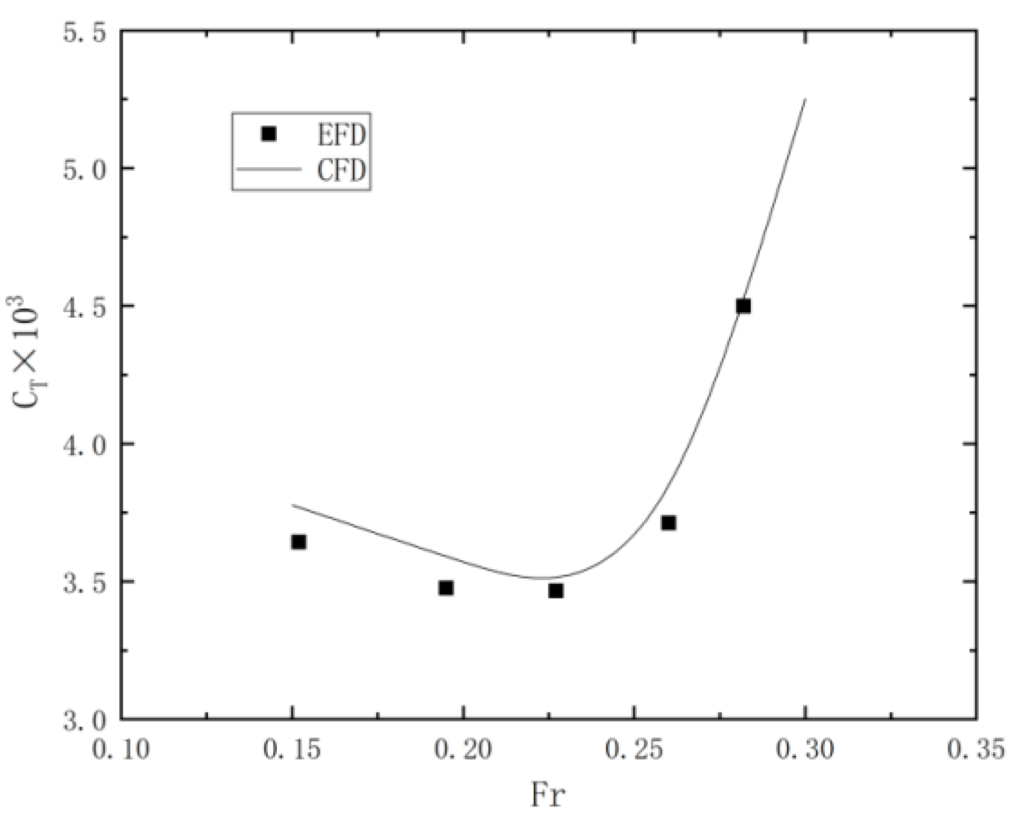
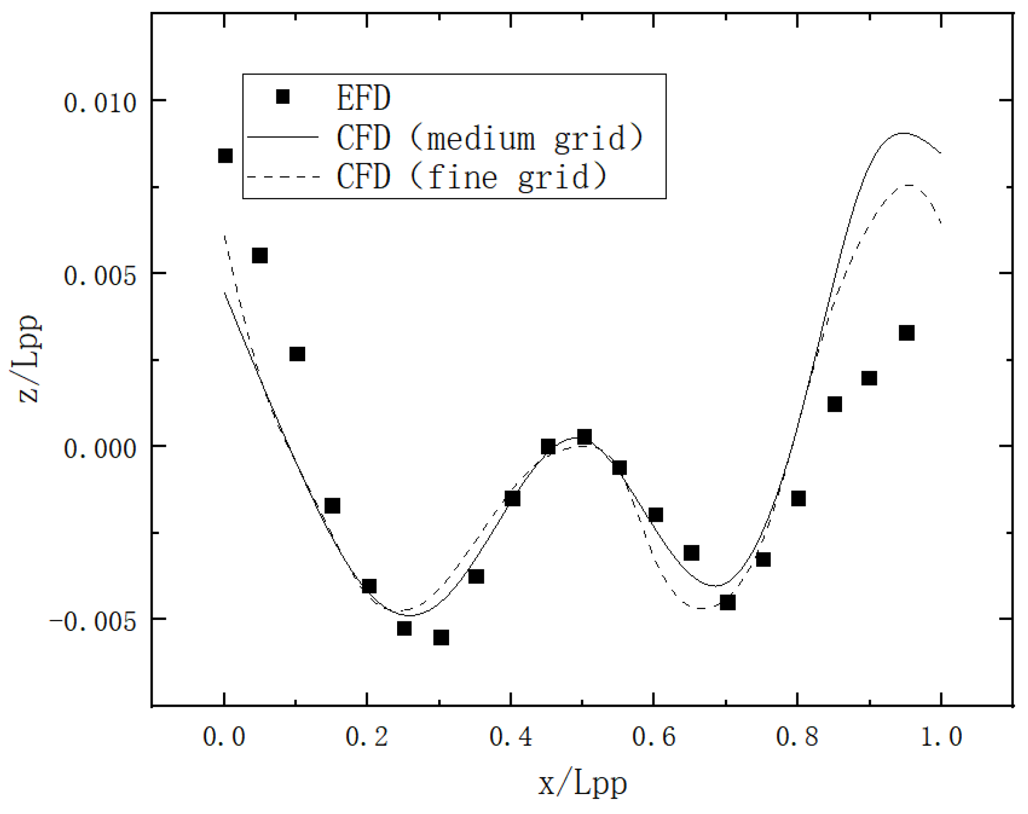
3.2. Verification and Validation

Verification is defined as a process for assessing simulation numerical uncertainty, and validation is defined as a process for assessing simulation modelling uncertainty [32]. Grid convergence verification is performed according to Celik et al. [33]. Three kinds of grids are selected; the numbers of the grids (N₁, N₂, N₃) are 4,453,641, 2,210,936 and 1,045,682; the calculation working condition is selected as Fr = 0.26; and the hull model allows pitch and heave. The refinement factors of the grids r₂₁ and r₂₃ and the order of discretization p are

$$r_{21}=\sqrt[3]{\frac{N_1}{N_2}}, r_{23}=\sqrt[3]{\frac{N_2}{N_3}}$$

(12)

$$p=\frac{1}{ln\left(r_{21}\right)}|ln|\frac{{\epsilon }_{32}}{{\epsilon }_{21}}|+q\left(p\right)|$$

(13)

$$q\left(p\right)=ln\left(\frac{r_{21}^p-s}{r_{32}^p-s}\right)$$

(14)

$$s=1\cdot sgn\left(\frac{{\epsilon }_{32}}{{\epsilon }_{21}}\right)$$

(15)

where ${\mathcal{E}}_{32}={\varphi }_3-{\varphi }_2$ ${\mathcal{E}}_{21}={\varphi }_2-{\varphi }_1$, and ${\varphi }_i$ are the simulation results for different number of grids. When s = 1, it indicates that the results show consistent convergence, and s = −1 indicates that the results show oscillatory convergence. The expression for extrapolated values ${\varphi }_{ext}^{21}$ is described as follows.

$${\varphi }_{ext}^{21}=\frac{r_{21}^p{\varphi }_1-{\varphi }_2}{r_{21}^p-1}$$

(16)

Approximate errors $e_a^{21}$ and extrapolated relative errors $e_{ext}^{21}$ are defined as

$$e_a^{21}=\left|\frac{{\varphi }_2-{\varphi }_1}{{\varphi }_1}\right|$$

(17)

$$e_{ext}^{21}=\left|\frac{{\varphi }_{ext}^{12}-{\varphi }_1}{{\varphi }_{ext}^{12}}\right|$$

(18)

the convergence index $GC{I}_{\mathit{fine}}^{21}$ of the fine mesh is obtained by the following expression.

$$GC{I}_{fine}^{21}=\frac{1.25e_a^{21}}{r_{21}^p-1}$$

(19)

The verification of the results of the resistance coefficient calculation was carried out according to the above equation, where p can be solved using fixed-point iteration. The results of the calculations are shown in the

Table 2. Calculation of the grid-independent verification.

Form	Value
r21	1.26
r23	1.28
φ1	0.003751
φ2	0.003784
φ3	0.004064
ε32	0.00028
ε21	0.000033
s	1
q	−0.1650
p	9.0759
$e_a^{21}$	0.008798
${GCI}_{fine}^{21}$	0.001502

. According to Table 2, it can be seen that the numerical uncertainty of the resistance coefficient of the simulation is 0.15%, which is less than 2%

The resistance coefficients (C_T) of the KCS ship are calculated and compared with the experimental data, as shown in

Table 3. Validation of the resistance coefficients.

Number of Grids	CT	Errors
4,453,641	0.003751	1.074%
2,210,936	0.003784	1.952%
1,045,682	0.004064	9.497%

. In CFD studies, under the premise of guaranteeing the computational accuracy, the medium mesh scheme is generally chosen to be similar to the results of the fine mesh scheme [34]. It can be seen that the numerical simulation results of medium and fine grids are closer to that of the experiment, but the effect of fine grid on the accuracy of the results is limited. In order to take into account the computational accuracy and computational time, the following numerical simulations in this study are carried out using medium grids.

Figure 3 shows the comparison between the resistance coefficient of KCS with different Fr and the experimental value [35] when the medium grid is used. Figure 4 shows the wave height along the hull surface when Fr = 0.26, which is obtained by using the medium grid, and the comparison with the experimental data [36]. For the resistance coefficients, the CFD results are overall slightly larger than the EFD results, and the error decreases with increasing speed. For the wave height along the hull surface, the CFD results for the medium grid are very close to the EFD results at the midship section. However, the CFD results are smaller than the EFD results at the stern, and the opposite is true at the bow. The fine-grid results are closer to the EFD results at the bow and stern, but the overall difference is not much different from that of the medium-grid results.

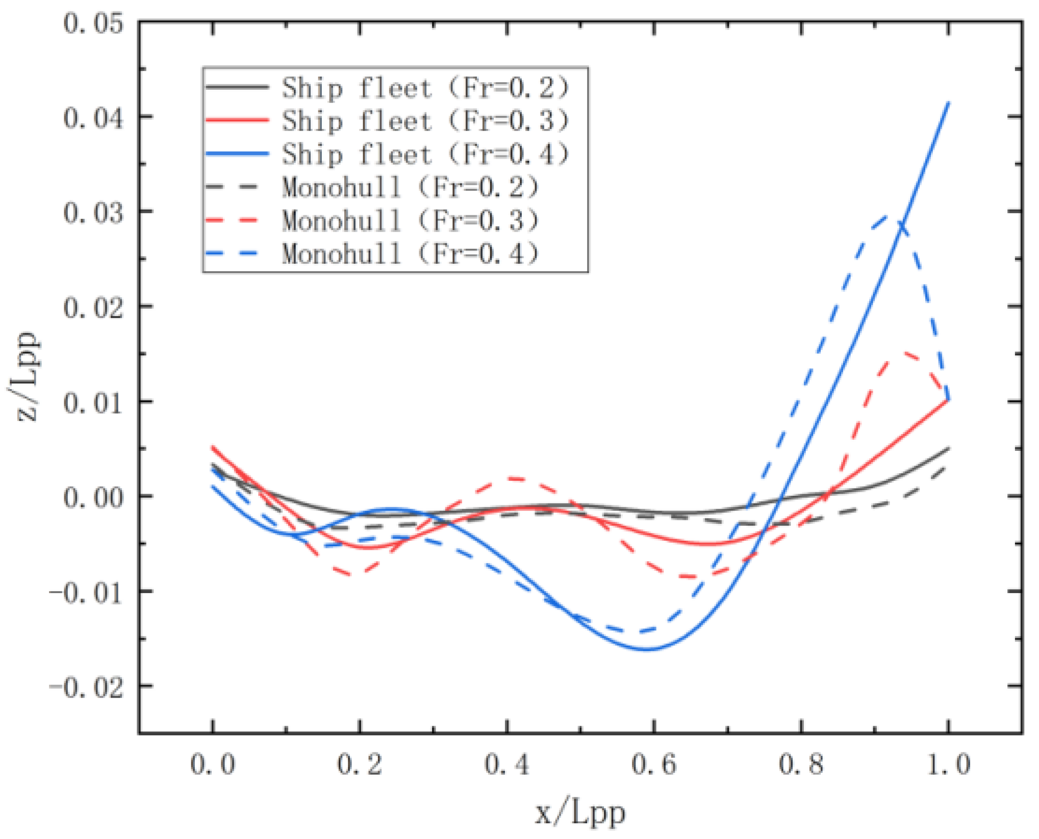
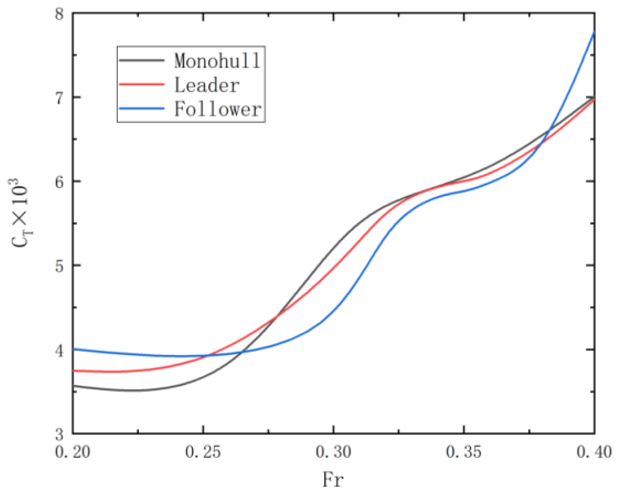
3.3. Hydrodynamic Interactions between Two Ships

Two KCS ships with the same parameters are set up in the flow field, and the two ships follow forward and backward at the same speed and keep the interval not changing with time. The intersection point of the middle axis of the rudder bar of the following ship and the water surface is taken as the coordinate origin, and the axis direction and the computational domain settings are the same as in the case of a single ship. The unfactorized interval is defined as l = D/L, where D is the distance between the intersection point of the middle axis of the leading ship’s rudder bar and the water surface and the coordinate origin, and L is the overall length of the ship. Figure 5 shows the flow fields for the monohull case and the two-ships case at l = 1.1 and different Fr.

As shown in Figure 5, Figure 6 and Figure 7, the flow field exhibits different characteristics at different Fr. For the monohull case, it can be found that the transverse wave has the largest amplitude in the y = 0 plane, and the amplitude gradually decreases along the direction away from the stern. When Fr = 0.3, the second and third wave heights after the ship are 55.8% and 39.0% of the first wave height, respectively. The higher the speed of the ship, the more intense the flow field behind the ship, which is manifested in larger wave amplitude, longer wavelength, and farther propagation range [37]. As shown in Figure 5, when Fr = 0.4, the highest wave peak can be observed, but when Fr = 0.2, the transverse wave only shows a slight disturbance at the stern. Generally speaking, the Kelvin wave consists of the superposition of the transverse wave propagating away from the stern and the divergent wave propagating toward the sides. Different superposition ratios affect the pattern of the Kelvin wave. Transverse waves dominate when the ship’s speed is low, and divergent waves dominate when the ship’s speed is high, as shown in Figure 6. When Fr = 0.3, the wavelength of the rising wave behind the ship is about 0.53 times the length of the ship, but when Fr = 0.4, the wavelength is about 0.92 times the length of the ship. When Fr = 0.2, the range of influence of the ship’s hull on the flow field behind it is very limited, and the wavelength and wave height are small. When Fr = 0.3, it can be observed that the transverse wave is more noticeable, the wavelength increases, and the propagation range increases. When Fr = 0.4, although the overall wave height increases, the percentage of transverse waves decreases, and the divergent waves in the flow field are more obvious, which are characterized by spreading to both sides.

As shown in Figure 5 and Figure 7, the change rule of the flow field behind the following ship in the two-ships case with speed is similar to the monohull case. When Fr = 0.3, the wavelength of the rising wave behind the ship is about 0.58 times the length of the ship, and when Fr = 0.4, the wavelength is about 0.90 times the length of the ship, which is similar to the monohull case. But the difference is that the transverse wave amplitude is more obvious at low speed (Fr = 0.2), which may be due to the fact that the disturbing effect of the ship fleet on the flow field is stronger than that in the monohull case.

The wave height along the hull surface of the monohull case and the follower under different Fr are obtained, as shown in Figure 8. It can be found that the higher the ship’s speed, the more intense the change of the flow field around the ship is, and the wavelength is longer. When Fr = 0.2, the hull surface wave is very small, and when Fr = 0.4, the wave amplitude increases dramatically compared with the low-speed condition, and higher wave peaks at the bow and stern as well as lower troughs in the middle of the ship can be observed. For the monohull case the maximum wave height at the bow of the ship reaches 0.03022 L_pp(m), and the depth of the trough at the middle of the ship is 0.01456 L_pp(m).

As shown in Figure 8, the wave height along hull surface of the following ship is quite different from that in the monohull case; when Fr = 0.3, the surface wave amplitude of the hull of the two-ships case is significantly reduced compared with that of the monohull case, but the opposite phenomenon occurs when Fr = 0.4, and larger wave peaks and troughs are observed at the bow and the middle of the ship, respectively, which suggests that the influence of the leading ship on the following ship exhibits different characteristics at different speeds. When Fr = 0.3, the depth of trough at midship is 0.00877 L_pp(m) and 0.00575 L_PP(m) for the monohull case and the following ship of the fleet case, respectively, and the depth of trough at midship is reduced by 34.4% for the following ship under the influence of the leading ship. But when Fr = 0.4, the depth of trough at midship is 0.01456 L_PP(m) and 0.01775 L_PP(m) for the monohull case and the following ship of the fleet case, respectively, and the depth of trough at midship is increased by 21.9% for the following ship under the influence of the leading ship. At the same time, the peaks and troughs appear in different locations.

When a ship sails on the surface of the water, the bow exerts pressure on the water surface, setting off a set of waves that follow the ship forward, called the bow wave. At this time, the bow part of the ship is a high-pressure area. The stern part of the ship will also set off a group of waves with the ship forward, called the stern wave. At this time the stern part of the ship is a low-pressure area. Due to the pressure difference between the stern and the bow, the surface pressure distribution of the hull is not uniform, thus generating the wave resistance. There is a direct relationship between the magnitude of wave resistance and the speed. Figure 9 and Figure 10 show the resistance coefficients at different Fr and the change relative to the monohull case, where α is the percentage change in the resistance coefficient between the front and rear ship at different speeds compared to the monohull case. For the following ship, it can be seen that in a certain interval (0.27 < Fr < 0.38), the resistance of the following ship becomes smaller under the influence of the leading ship, and the reduction in resistance is greatest at Fr = 0.3; the resistance coefficient is reduced by 24.3%. However, when Fr > 0.38 or Fr < 0.27, the resistance of the following ship increases. The reason for this phenomenon may be that when the two ships sail forward and backward, the flow field around the following ship and the flow field behind the leading ship are superimposed on each other. When the transverse wave wavelength of the flow field at the stern of the leading ship is similar to the wavelength of the wave around the following ship and the phases are just canceled, the wave of the following ship is reduced, thus reducing the wave resistance of the following ship. On the contrary, it will increase the wave around the following ship, thus increasing the resistance of the following ship. When l = 1.1, the follower is close enough to have a significant impact on the resistance coefficient of the leader as well. When Fr is greater than 0.24, the resistance coefficients of the leader are all reduced compared to the monohull case, with the largest reduction occurring at Fr = 0.3, which is 13.2%. It shows that the interaction of the two ships can have a significant effect when the distance is close enough.

As shown in Figure 11, when Fr = 0.3, the waves around the following ship are reduced, so the resistance on it is greatly reduced. When Fr = 0.4, the waves around it are intensified and form a very high peak at the bow and a trough in the middle of the ship, thus increasing the resistance of the following ship. For the leading ship, at low speeds, the influence of the following ship is small and the resistance coefficient of the leading ship is very close to the monohull case. As the speed increases, the resistance of the leading ship decreases under the influence of the follower.

When l = 1.5, the wave height along hull surface of the following ship is shown in Figure 12. The resistance coefficient is shown in Figure 13. It can be found that with the increase in the interval between the two ships, the influence is greatly reduced. The influence of the resistance of the leading ship is significantly reduced, and in the case of l = 1.5, it is very close to the monohull case. The reason is that when l = 1.1, the following ship is very close to the leading ship, and the flow field disturbance caused by the bow of the following ship can still affect the flow field behind the leading ship. However, when l = 1.5, the influence area of the following ship’s bow is already far away from the leading ship’s stern area, so the influence is very limited. When the distance increases, the resistance coefficient of the follower is also weakened by the influence of the leader, which is due to the gradual decrease of the transverse wave amplitude of the wave along the direction away from its stern.

As in Figure 12, observing the wave heights on the surface of the ship for the monohull case and the two-ships case, we can find that the wave of the following ship is weakened for the two-ships case when Fr = 0.3. Also, in Figure 14 we can find that the resistance coefficient of the following ship is significantly reduced compared to the monohull case. The comparison of flow fields for monohull case and the two-ships case is shown in Figure 15. When Fr = 0.3, the depth of trough at midship is 0.00877 L_pp(m) and 0.00653 L_pp(m) for the monohull case and the following ship of the fleet case, respectively, and the depth of trough at midship is reduced by 25.5% for the following ship under the influence of the leading ship. When Fr = 0.3, the resistance coefficient of the follower is also reduced, and the size of the reduction is 13.75%. The influence of the resistance coefficient is greatly reduced for the leader, where the largest reduction is only 3.99%. For Fr = 0.4, the wave around the following ship is reduced, but the resistance coefficient is increased compared to the monohull case. This suggests that the influence of the rising wave is not the only factor affecting the resistance of the follower.

The change of followers compared to the monohull case is shown in

Table 4. Change of followers compared to the monohull case.

Fr	l	Amplitude at Midship	Resistance Coefficient
0.3	1.1	−34.4%	−24.3%
0.4	1.1	+21.9%	+3.2%
0.3	1.5	−25.5%	−13.75%
0.4	1.5	−40.2%	+11.0%

. According to the physical phenomenon of water resistance, ship sailing is divided into wave resistance, viscous pressure resistance, and friction resistance. Among them, the wave resistance is mainly due to the influence of waves, and the ship’s surface draft is different, thus generating a pressure difference. Therefore, when the wave height of the follower changes under the influence of the leader, the wave resistance it suffers will be different. The factors affecting the frictional resistance are mainly the wet surface area and speed of the ship. When the follower is in the wake field of the leader, the wet surface area of the follower will change due to the change of the wave height around the ship, and at the same time, due to the shading effect of the leader, the speed of the incoming current it suffers from is also reduced. For the viscous pressure resistance, the effect suffered by the follower is mainly reflected in the vortex generated by the hull and propeller of the leader. These are all important factors affecting the interference between ships, and the specific effects of these factors have yet to be studied.

4. Conclusions

It has been found that multiple ships following in formation in the form of a sea train can effectively reduce resistance. In this study, numerical simulation was carried out for the case of two ships following front and behind with the same speed, and it was compared with the monohull case. The change rule of resistance and flow field around the ship with the sailing speed and the distance between the two ships is analyzed, and the following conclusions are obtained:

(1)

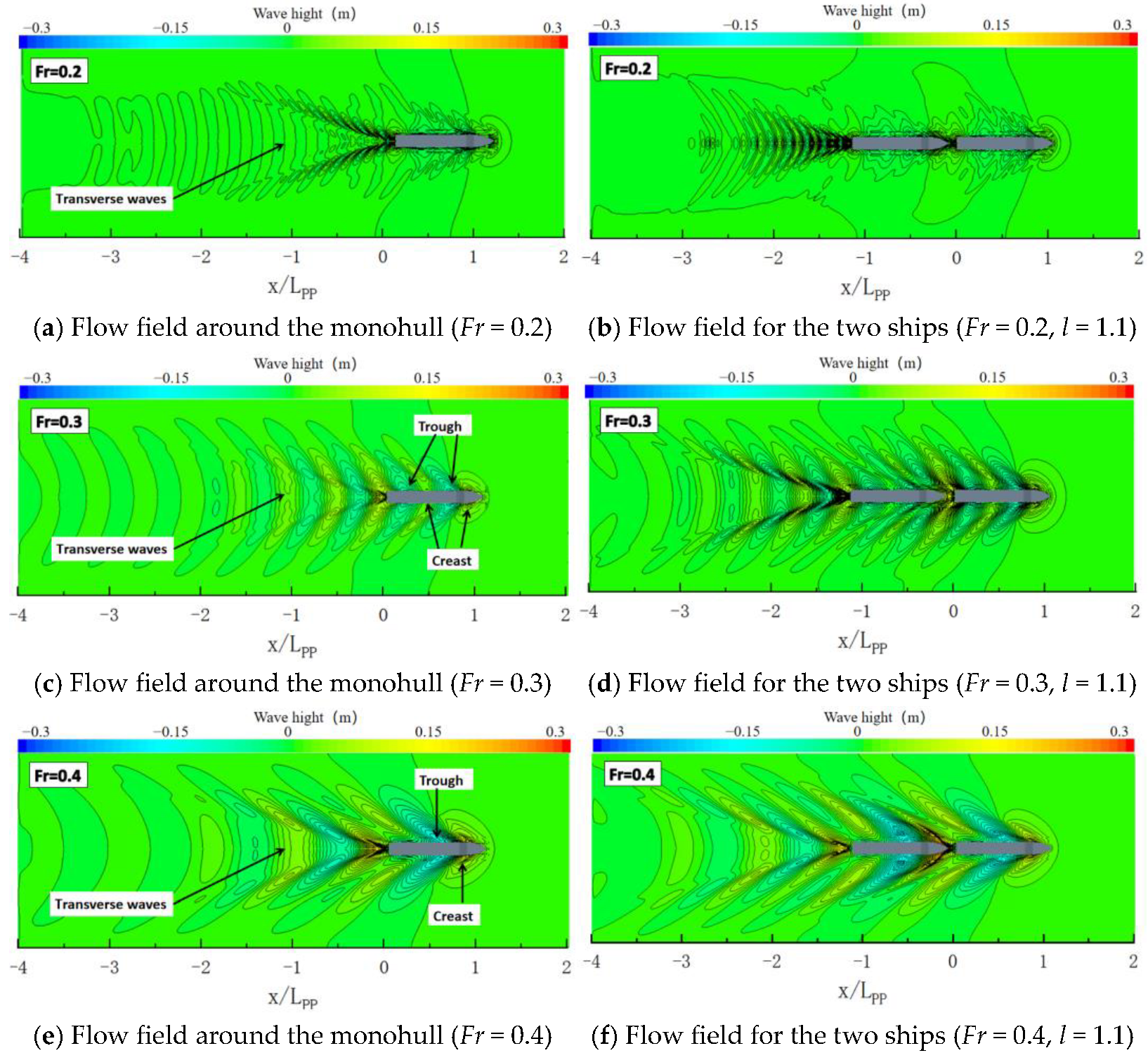
When a single ship is sailing in still water, the characteristics of the flow field are as follows: the wavelength and amplitude of the transverse wave increase with higher speed, and the flow field is more intense, but the ratio of the divergent wave in the flow field increases, and the ratio of the transverse wave decreases. When the speed increases, the amplitude and wavelength of the wave around the ship also increase accordingly.

(2)

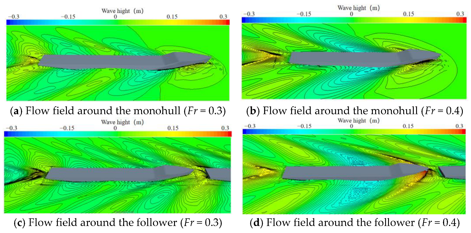
When the two ships follow each other, the flow field is characterized as follows: the amplitude of the transverse waveform of the following ship increases significantly at low speed compared with that of the monohull case. The wave around the ship is disturbed by the flow field of the leading ship and shows a different waveform from the monohull case. In the midship region of the following ship, the maximum reduction in wave amplitude can be as much as 40.2%.

(3)

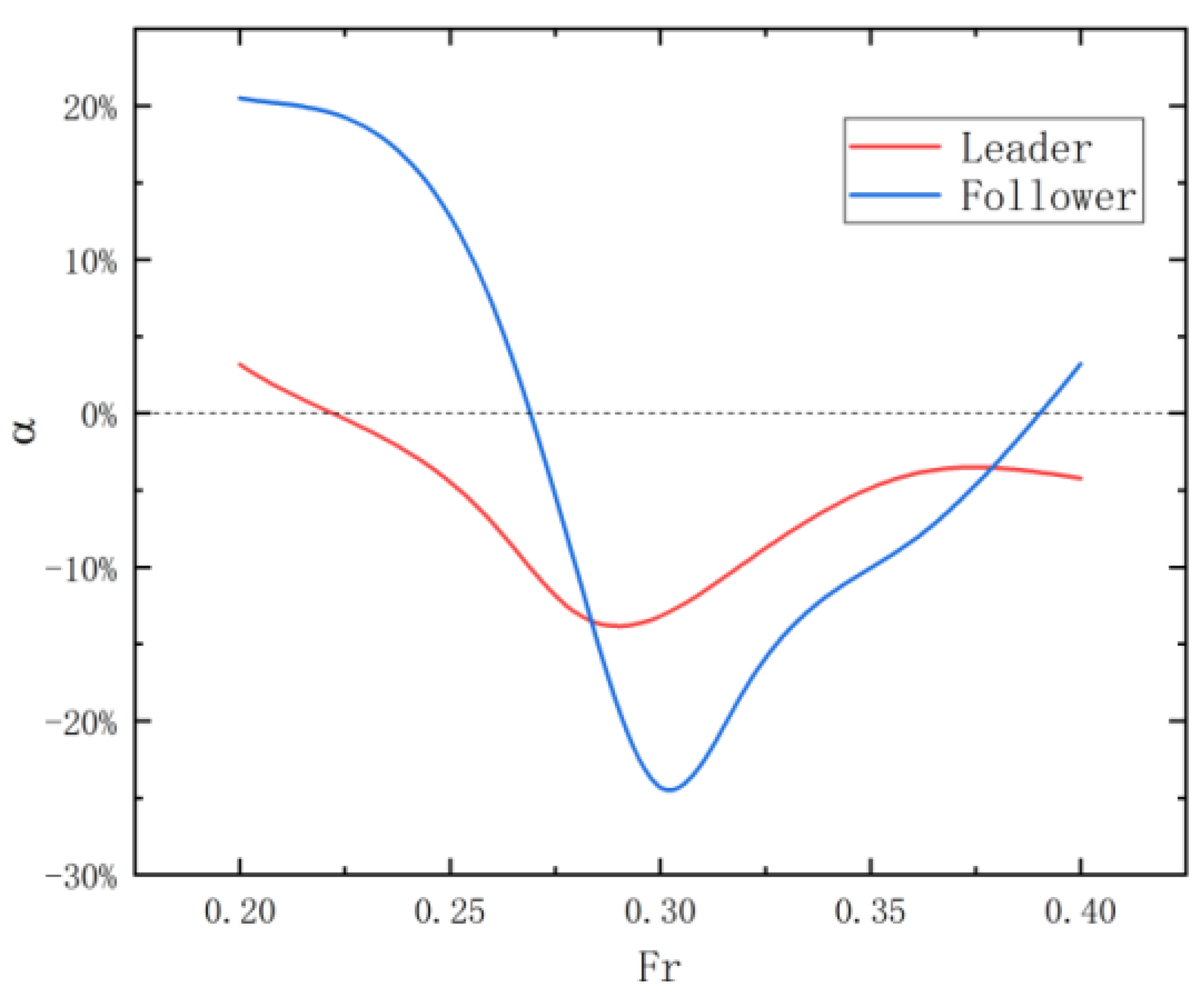
When the two ships follow at different speeds, their interactions are also different. In a certain speed interval, the resistance of the following ship is reduced due to the influence of the leading ship compared with the resistance of the monohull, where the maximum reduction can be up to 24.3%. By observing the flow field around the ship, the reason for this phenomenon may be that the transverse wave at the stern of the leading ship and the wave around the following ship are superimposed and interfere with each other. When the speed changes, the flow field behind the leading ship produces transverse waves with a specific wavelength range, which produces the effect of suppressing the amplitude of the wave around the follower, thus reducing the wave resistance of the following ship, and conversely the wave resistance will increase.

(4)

When the interval between the two ships increases, the impact between the two ships decreases, in which the impact on the leading ship decreases significantly and the impact on the following ship is also reduced to a certain extent.

The research of this study provides a reference for the case of two ships following each other, such as a fleet of ships, inter-ship supply, tugboat work, etc. When considering the above situation, we can choose a favorable interval and speed to reduce the resistance of the two ships.

References

1. Mizine, I.; Karafiath, G. Model Test Evaluation of High Speed Trimaran (HST) Sea Train Concept; SNAME: Alexandria, VA, USA, 2015. [Google Scholar]
2. Noblesse, F.; He, J.; Zhu, Y.; Hong, L.; Zhang, C.; Zhu, R.; Yang, C. Why can ship wakes appear narrower than Kelvin’s angle? Eur. J. Mech. B-Fluids 2014, 46, 164–171. [Google Scholar] [CrossRef]
3. Zhang, C.; He, J.; Zhu, Y.; Yang, C.-J.; Li, W.; Zhu, Y.; Lin, M.; Noblesse, F. Interference effects on the Kelvin wake of a monohull ship represented via a continuous distribution of sources. Eur. J. Mech. B-Fluids 2015, 51, 27–36. [Google Scholar] [CrossRef]
4. Darmon, A.; Benzaquen, M.; Raphael, E. Kelvin wake pattern at large Froude numbers. J. Fluid Mech. 2014, 738, R3. [Google Scholar] [CrossRef]
5. Pethiyagoda, R.; Moroney, T.J.; Lustri, C.J.; McCue, S.W. Kelvin wake pattern at small Froude numbers. J. Fluid Mech. 2021, 915, A126. [Google Scholar] [CrossRef]
6. Sun, X.; Cai, M.; Wang, J.; Liu, C. Numerical Simulation of the Kelvin Wake Patterns. Appl. Sci. 2022, 12, 6265. [Google Scholar] [CrossRef]
7. Zhou, J.; Ren, J.; Bai, W. Survey on hydrodynamic analysis of ship–ship interaction during the past decade. Ocean Eng. 2023, 278, 114361. [Google Scholar] [CrossRef]
8. Xueqian, Z.; Sutulo, S.; Guedes Soares, C. Computation of ship hydrodynamic interaction forces in restricted waters using potential theory. J. Mar. Sci. Appl. 2012, 11, 265–275. [Google Scholar] [CrossRef]
9. Du, P.; Ouahsine, A.; Sergent, P. Influences of the separation distance, ship speed and channel dimension on ship maneuverability in a confined waterway. Comptes Rendus Méc. 2018, 346, 390–401. [Google Scholar] [CrossRef]
10. Luo-Theilen, X.; Rung, T. Computation of mechanically coupled bodies in a seaway. Ship Technol. Res. 2017, 64, 129–143. [Google Scholar] [CrossRef]
11. Wang, J.F. Numerical Simulation of Hydrodynamic Interactions between Two Ships in Underway Replenishment at Sea. Ph.D. Thesis, Harbin Engineering University, Harbin, China, 2005. [Google Scholar]
12. Harada, T.; Nakashima, A.; Arai, M.; Nishimoto, K. Motions and safety of a floating liquefied natural gas and shuttle tanker during side-by-side offloading operations. Proc. Inst. Mech. Eng. Part M J. Eng. Marit. Environ. 2018, 233, 610–621. [Google Scholar] [CrossRef]
13. Li, A.; Zhang, G.; Liu, X.; Yu, Y.; Zhang, X.; Ma, H.; Zhang, J. Hydrodynamic Characteristics at Intersection Areas of Ship and Bridge Pier with Skew Bridge. Water 2022, 14, 904. [Google Scholar] [CrossRef]
14. Vasudevan, N.; Seeninaidu, N. CFD simulation of the passing vessel effects on moored vessel. Ships Offshore Struct. 2019, 15, 184–199. [Google Scholar] [CrossRef]
15. Wnęk, A.D.; Sutulo, S.; Guedes Soares, C. CFD Analysis of Ship-to-Ship Hydrodynamic Interaction. J. Mar. Sci. Appl. 2018, 17, 21–37. [Google Scholar] [CrossRef]
16. Ekerhovd, I.; Ong, M.; Taylor, P.; Zhao, W. Numerical study on gap resonance coupled to vessel motions relevant to side-by-side offloading. Ocean Eng. 2021, 241, 110045. [Google Scholar] [CrossRef]
17. Li, B. Multi-body hydrodynamic resonance and shielding effect of vessels parallel and nonparallel side-by-side. Ocean Eng. 2020, 218, 108188. [Google Scholar] [CrossRef]
18. Yuan, Z.-M.; Li, L.; Yeung, R. Free-Surface Effects on Interaction of Multiple Ships Moving at Different Speeds. J. Ship Res. 2019, 63, 251–267. [Google Scholar] [CrossRef]
19. Li, M.-X.; Yuan, Z.-M.; Tao, L. An iterative time-marching scheme for the investigation of hydrodynamic interaction between multi-ships during overtaking. J. Hydrodyn. 2021, 33, 468–478. [Google Scholar] [CrossRef]
20. Yuan, Z.-M.; Chen, M.; Jia, L.; Ji, C.; Incecik, A. Wave-riding and wave-passing by ducklings in formation swimming. J. Fluid Mech. 2021, 928, R2. [Google Scholar] [CrossRef]
21. Ma, C.; Zhao, X.; Cheng, X.; Yang, Y.; Fan, L. The wave interference and the wave resistance of a leader-follower ship fleet. Ocean Eng. 2023, 274, 114089. [Google Scholar] [CrossRef]
22. Ferziger, J.; Perić, M.; Street, R. Computational Methods for Fluid Dynamics; Springer: Berlin/Heidelberg, Germany, 2020. [Google Scholar]
23. Wilcox, D. Turbulence Modeling for CFD, 3rd ed.; Hardcover; DCW Industries: La Cañada, CA, USA, 2006. [Google Scholar]
24. Quérard, A.; Temarel, P.; Turnock, S. Influence of Viscous Effects on the Hydrodynamics of Ship-Like Sections Undergoing Symmetric and Anti-Symmetric Motions, Using RANS. In Proceedings of the International Conference on Offshore Mechanics and Arctic Engineering, Estoril, Portugal, 15–20 June 2008; Volume 5. [Google Scholar]
25. Gorman, J.; Bhattacharyya, S.; Cheng, L.; Abraham, J. Turbulence Models Commonly Used in CFD; Intech Open: London, UK, 2021. [Google Scholar]
26. Shih, T.H.; Liou, W.; Shabbir, A.; Yang, Z.; Zhu, J. A New k-(Eddy Viscosity Model for High Reynolds Number Turbulent Flows-Model Development and Validation. Comput. Fluids 1994, 24, 227–238. [Google Scholar] [CrossRef]
27. Hirt, C.W.; Nichols, B.D. Volume of fluid (VOF) method for the dynamics of free boundaries. J. Comput. Phys. 1981, 39, 201–225. [Google Scholar] [CrossRef]
28. International Towing Tank Conference (ITTC). Practical guidelines for ship CFD applications. In Proceedings of the 26th ITTC, Rio de Janeiro, Brazil, 28 August–1 September 2011. [Google Scholar]
29. Tezdogan, T.; Demirel, Y.K.; Kellett, P.; Khorasanchi, M.; Incecik, A.; Turan, O. Full-scale unsteady RANS CFD simulations of ship behaviour and performance in head seas due to slow steaming. Ocean Eng. 2015, 97, 186–206. [Google Scholar] [CrossRef]
30. CD-Adapco. User Guide STAR-CCM+, Version 9.0.2; Siemens: Berlin, Germany, 2014.
31. Khan, N.; Ibrahim, Z.; Ashfaq Ali, M.; Jameel, M.; Khan, M.; Javanmardi, A.; Oyejobi, D. Numerical simulation of flow with large eddy simulation at Re = 3900: A study on the accuracy of statistical quantities. Int. J. Numer. Methods Heat Fluid Flow 2019, 30, 2397–2409. [Google Scholar] [CrossRef]
32. ITTC. Uncertainty Analysis in CFD Verification and Validation Methodology and Procedures. In Proceedings of the Resistance Committee of 25th ITTC, Fukuoka, Japan, 14–20 September 2008. [Google Scholar]
33. Celik, I.; Ghia, U.; Roache, P.J.; Freitas, C.; Coloman, H.; Raad, P. Procedure of Estimation and Reporting of Uncertainty Due to Discretization in CFD Applications. J. Fluids Eng. 2008, 130, 078001. [Google Scholar] [CrossRef]
34. Liu, M.-M.; Wang, H.-C.; Shao, F.-F.; Jin, X.; Tang, G.-Q.; Yang, F. Numerical investigation on vortex-induced vibration of an elastically mounted circular cylinder with multiple control rods at low Reynolds number. Appl. Ocean Res. 2022, 118, 102987. [Google Scholar] [CrossRef]
35. Larsson, L.; Stern, F.; Visonneau, M. Numerical Ship Hydrodynamics—An Assessment of the Gothenburg 2010 Workshop; Springer Science+Business Media: Berlin, Germany, 2014. [Google Scholar]
36. Kim, W.J.; Van, S.H.; Kim, D.H. Measurement of flows around modern commercial ship models. Exp. Fluids 2001, 31, 567–578. [Google Scholar] [CrossRef]
37. Du, P.; Ouahsine, A.; Sergent, P. Hydrodynamics prediction of a ship in static and dynamic states. Coupled Syst. Mech. 2018, 7, 163–176. [Google Scholar] [CrossRef]
Figure 1. Computational domain and the boundary conditions.
Jmse 12 00056 g001
Figure 2. Medium grid for the monohull case and the two-ships case.
Jmse 12 00056 g002
Figure 3. CFD and EFD resistance coefficients for medium grids.
Jmse 12 00056 g003
Figure 4. Wave height along the hull surface of CFD and EFD for medium grids and fine grids.
Jmse 12 00056 g004
Figure 5. Flow fields for the monohull case and the two-ships case at l = 1.1 and different Fr.
Jmse 12 00056 g005
Figure 6. Transverse wave in the y = 0 plane behind the monohull.
Jmse 12 00056 g006
Figure 7. Transverse wave in the y = 0 plane behind following ship (l = 1.1).
Jmse 12 00056 g007
Figure 8. Wave height along hull surface of the monohull case and the follower at different Fr (l = 1.1).
Jmse 12 00056 g008
Figure 9. Resistance coefficient (l = 1.1).
Jmse 12 00056 g009
Figure 10. Change in resistance coefficient relative to monohull case (l = 1.1).
Jmse 12 00056 g010
Figure 11. Comparison of flow fields (l = 1.1).
Jmse 12 00056 g011
Figure 12. Wave height along hull surface of the following ship at different Fr (l = 1.5).
Jmse 12 00056 g012
Figure 13. Resistance coefficient (l = 1.5).
Jmse 12 00056 g013
Figure 14. Change in resistance coefficient relative to monohull case (l = 1.5).
Jmse 12 00056 g014
Figure 15. Comparison of flow fields for monohull case and the two-ships case (l = 1.5).
Jmse 12 00056 g015