Abstract
This paper presents an optimal output-feedback tracking control problem for multiple unmanned marine vehicles (UMVs) to track a desired trajectory. To guarantee the control objective in an optimal manner, adaptive dynamic programming (ADP) with optimal compensation terms is adopted. A neural velocity observer is designed based on a neural network (NN) to estimate the unmeasured system states and the unknown system dynamics. Furthermore, a disturbance observer (DO) is proposed to go against the effect of the unknown external disturbance of the sea environment. It is proved that the proposed controller can guarantee that all signals in the closed-loop system are bounded. Simulation results are given to demonstrate the effectiveness of the proposed control algorithm.
1. Introduction
In recent years, unmanned marine vehicles (UMVs) have garnered increasing attention for the exploration of natural resources in oceanic spaces due to their unique advantages, such as low energy costs and advanced intelligence. Furthermore, UMVs can complete dangerous tasks without putting human lives at risk [1,2]. However, a solitary UMV may not suffice to execute complex tasks in some situations. Thus, the control problem of multiple UMVs has garnered substantial interest. In recent years, the coordinated control of multiple UMVs has become a burgeoning research topic [3]. Some important theoretical results of coordinated control of multiple vehicles have been reported [4,5,6,7,8]. In [8], a time-varying formation control problem was presented. Connectivity preservation and collision avoidance were investigated with position-heading measurements. In [5], the path-tracking control of under-actuated unmanned surface vehicles was investigated. Model uncertainties and unknown disturbances over a wireless network were considered. This research has far-reaching implications; however, the control attempts can use high amounts of energy because the aforementioned control design strategies do not consider the optimization problem.
Optimal control is a fundamental design principle that can be adopted to enhance the control performance of dynamic systems. Given that ocean transportation or deep-sea exploration frequently necessitates substantial energy provision, it becomes imperative to incorporate optimization into vessel control design to reduce energy consumption. However, the optimal control of UMVs is a difficult problem due to the inherent nonlinearities of the UMV system. The optimization problems of nonlinear systems often need to solve the Hamilton–Jacobi–Bellman (HJB) equation, which does not have a closed-form solution. To handle this difficulty, a promising adaptive optimal method was presented based on the reinforcement learning (RL) method, namely, adaptive dynamic programming (ADP) [9,10,11,12], in which an RL system was designed to approximate the HJB equation [13,14,15]. Many studies on the control problems of vehicles by using the ADP method have been reported [16,17,18]. In [16], the optimal tracking control problem for the dynamic positioning of marine vessels was investigated. The observer based on a fuzzy logic system (FLS) was given to handle the problem of unmeasured states of the vessels. A disturbance observer (DO) was given to estimate the external disturbances. In [17], a data-driven RL-based controller was introduced to address the optimal control problem of the vehicle. Using a data-driven approach, a model-free control method was formulated to achieve control optimality and prescribed tracking accuracy concurrently. In [18], an optimal control scheme was presented for RL-based optimal tracking control applied to UMVs. The unknown dead-zone input nonlinearities and unknown disturbances were considered and handled by using a neural network (NN)-based identifier. This research shows how the optimal control problem of a single UMV can be solved. However, the optimal tracking control problem of multiple UMVs cannot be handled directly using these methods.
In practical applications, accurately obtaining velocity information from shipborne sensors is often challenging due to the potential impact of noise interference and sensor signal loss on its effectiveness [19]. To handle this difficulty, some research based on the observer has been reported [3,20,21,22]. In [20], a study on the distributed containment maneuvering problem was conducted. Adopting the input–output data from each vehicle, a novel approach utilizing an echo state network-based observer was introduced to address the issue of unmeasured states. In [3], the flocking control problem of vehicles was studied. The velocity information of the vehicles was obtained by employing an extended state observer. In [22], the path-following problem of vehicles was studied. Unmeasured states were handled by giving a state observer based on FLS. From the studies mentioned above, establishing an observer to handle the unmeasured velocity information of vehicles is an effective approach.
When working in a sea environment, the control effectiveness of a UMV can be influenced by external disturbances such as wind and waves, which may lead to a failure to achieve the control target [23,24]. Thus, it is important to adopt disturbance rejection techniques to reduce the effect of unknown external disturbances. In recent years, many disturbance observer (OB)-based controllers were reported [24,25,26]. In [24], the robust leader–follower synchronization navigation for the UMVs was presented. The problem of unknown external disturbance was solved by adopting OB. In [26], the trajectory tracking control problem of UMVs was solved using the dynamic surface control technique. The time-varying disturbances were considered and estimated by a proposed DO. These results are fruitful and inspiring.
Motivated by the observations described above, the formation tracking problem of multiple UMVs is studied in this paper. An ADP algorithm with an optimal compensation term is adopted to guarantee the control objective optimally. An adaptive controller is designed using the backstepping technique; the optimal tracking control problem is transformed into an equivalent optimal regulation problem. Subsequently, an optimal compensation term is designed by using the policy iteration method. The overall optimal control input is the adaptive controller plus the optimal compensation term. To handle the unknown time-varying external disturbances of the sea environment, a DO is designed. It is proved that the proposed controller can guarantee that all signals in the closed-loop system are bounded. Simulation results are given to demonstrate the effectiveness of the proposed control algorithm.
The main contribution of this work can be summarized as follows.
(1) Unlike the references [4,5,6,7,8] investigating the tracking control problem of multiple UMVs without consideration of optimality, this paper considers optimality for designing the consensus controller. This means that the control method proposed in this paper can achieve the tracking control target with less energy consumption.
(2) Compared with the works in [17,18], an advantage of this paper is that this paper investigated the optimal tracking control problem of multiple UMVs. In contrast, the authors in [17,18] only investigated the optimal tracking control problem of a single UMV. Therefore, the task we set out to achieve is more challenging than the existing studies.
The rest of the paper is organized as follows: Section 2 provides the problem formulation, Section 3.1 presents the DO, Section 3.2 and Section 3.3 introduce the adaptive controller and the optimal compensation term, Section 3.4 provides a stability analysis, Section 4 provides the simulation results, and Section 5 presents concluding remarks.
2. Problem Formulation
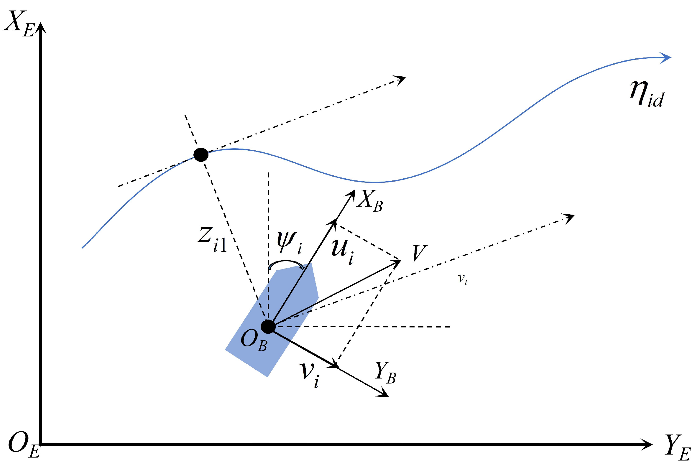
Two reference frames are adopted: a body-fixed reference frame (BF) and a north-east-down reference frame (NED), which can be found in Figure 1. These two reference frames are generally adopted in ship motion control, and readers can find more details in [27,28,29].

Figure 1.
Illustration of the coordinations in NED () and BF ().
Considering the leader–follower formation control problem of m UMVs, the underactuated system dynamics of 3 degrees of freedom (3-DOF) with uncertain dynamics can be described as follows [28,29,30]:
where , is the position of UMV in the earth-fixed frame, is the heading angle in the earth-fixed frame, denotes the velocities of UMV in the body-fixed frame, and denotes the control input. denotes the uncertain dynamics. is the unknown disturbance from the sea environment. is the rotation matrix from the earth-fixed frame to the body-fixed frame, which is given as follows:
is an inertia matrix including hydrodynamic added inertia; is the damping matrix; is a matrix of the centripetal and Coriolis terms. These three terms are shown as follows:
where , , , , and . denotes the mass of the vessel, and denotes the distance between the center of gravity of the vessel and the origin of the body-fixed frame. is the moment of inertia. , , , , and . , , and are the corresponding hydrodynamic derivatives. Consider a virtual leader moving along a desired trajectory shown as .
For simplicity, we can obtain the following equation by using System (1):
where
and
is an unknown function since is unknown. To handle this problem, NN is adopted to obtain the approximation.
Control Problem Statement: This study aims to design an output feedback control algorithm that can handle the optimal tracking control problem of multiple UMVs with unknown external disturbance and uncertain dynamics. The controller can ensure that all the signals in the closed-loop are bounded.
3. Main Results
3.1. Neural Observer Design
A neural state observer (NSO) is adopted to handle the unmeasured velocities and unknown system dynamics. From (4), we can obtain the following equations:
where , , , , , , , . Since is unknown, NN is adopted to obtain the approximation, which can be described as
denotes the minimum approximation error, i.e., , where is a constant vector, . We can obtain the approximation of as
We can design the neural velocity observer as follows:
where , , and . , , . , , and are a Hurwitz matrix by choosing the suitable parameters , , , , , and . , , , , , and are positive definite matrices that satisfy , , and , where , , and . is the disturbance estimation that the DO will obtain. Let be the disturbance approximation error. Define the NSO error dynamics as , , and . From (7) and (10), we can obtain the error dynamics of NSO as follows:
3.2. Disturbance Observer Design
To implement the DO, we begin by defining the auxiliary vector for each vehicle as follows:
where , and a positive definite design matrix is employed. We can obtain the time derivative of as
Since is unknown, is also unknown. We can obtain an approximation of using the following equation:
Thus, we obtain as follows:
Let . The time derivative of is described as follows:
3.3. Adaptive Controller Design
The proposed adaptive controller is designed utilizing the backstepping technique. First, the change of coordinates is given as follows:
where , and represents the tracking trajectory of the leader. Here, , where and denote the relative position between the i-th ASV and the leader in the and directions, respectively. serves as the virtual control for design purposes, where and are the adaptive virtual control and the optimal compensation term, respectively. The actual control combines these two terms, i.e., .
From (17), we can obtain the following:
To obtain the control objective, we design the following equation:
We can obtain the following:
By using Young’s inequality, we can obtain the following:
The adaptive controller can be designed as follows:
where is the positive design parameter vector. Thus, we can obtain the following:
where , , .
We design the following Lyapunov function:
Utilizing the fact that , we can obtain the following equation:
By applying Young’s inequality, the following inequalities can be obtained:
and
We define , where , and one has
We can design the adaptive controller and adaptive law as follows:
and
where is the positive design vector. According to Young’s inequality, we can obtain that
and
From (17) and (18), the tracking error dynamics can be described as follows:
where , , , . The cost function of the tacking error system can be described as
where is the optimal index, is a positive definite matrix satisfying only if and for , , , and are positive bounds. is a positive definite matrix. An infinitesimal equivalent of (43) can be written as follows [31]:
We define a Hamiltonian function as
where is the associated admissible control, and is the gradient of with regard to . The optimal controller can be obtained by applying the condition , and one has
where represents the gradient of with respect to . The HJB equation can be described as follows:
with . It can be concluded that is a continuously differentiable and radially unbounded Lyapunov function, and the derivative with an optimal controller can be described as
By choosing suitable satisfying and , the following equation can be obtained [32]:
From (37), (40), and (41), we can obtain that
where . According to (49), it can be seen that becomes negative when the controller is designed by adopting the optimal control method to stabilize the tracking error system (42), which implies that the tracking error remains bounded and the cost function is minimized. However, the HJB Equation (47) is difficult to solve, so the ADP method is applied in the next section to obtain .
3.4. Optimal Compensation Term Design
To obtain the approximation of the optimal cost function, NN is adopted as
Here, represents the ideal parameter, denotes the basis function, and signifies the minimum approximation error. The gradient of the optimal cost function is given by
where and are the gradients of and , respectively. The optimal controller and the Hamiltonian function are expressed below:
We can obtain the following equation:
Describing the approximation of the optimal cost function achieved by NN, we have
where is the approximation of . The optimal controller estimation can be reformulated as follows:
The approximate Hamiltonian function can be obtained as follows:
where , , .
We choose the weight updating law of as follows:
The estimation error of the optimal cost function parameter is defined as . From this definition, we can obtain that
The error dynamics of Equation (59) can be expressed as follows:
where .
3.5. Stability Analysis
Theorem 1.
For the multiple UMV systems (System (1)), the weight updating law is given by (39), the adaptive controller is defined by (38), the optimal compensation term is provided by (57), and the updated law for the cost function is specified by (59). By selecting the design parameters appropriately, the entire control scheme ensures the boundedness of all signals in the closed-loop system, and the system outputs can optimally track the reference signal.
Proof.
Consider the following Lyapunov function:
We can obtain that
Assume that , , , and , where , , , and are positive constants. By applying Young’s inequality and the Cauchy–Schwartz inequality to (63), we can obtain the following inequality:
where
Assume the following equations hold:
or
or
or
or
or
or
Thus, according to standard Lyapunov extension [31], we can obtain , and all signals within the closed-loop system remain bounded. □
4. Simulations and Comparison Study
4.1. Simulation Experiment
The simulation is applied by using MatlabR2018a. The parameter of CyberShip II is adopted in the simulation part; the details of this simulation model can be found in [33]. Three UMVs are adopted in the simulation experiment, which are named , , and , respectively. is designed as . The initial position of the three UMVs are , , , and , respectively. The parameters of related position are given as follows: , , , , , , , and . , and . The applied disturbances are chosen as follows: , , and . The desired tracking signal of the virtual leader is given as .
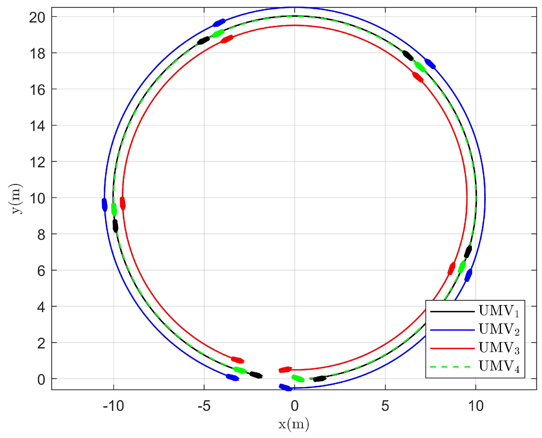
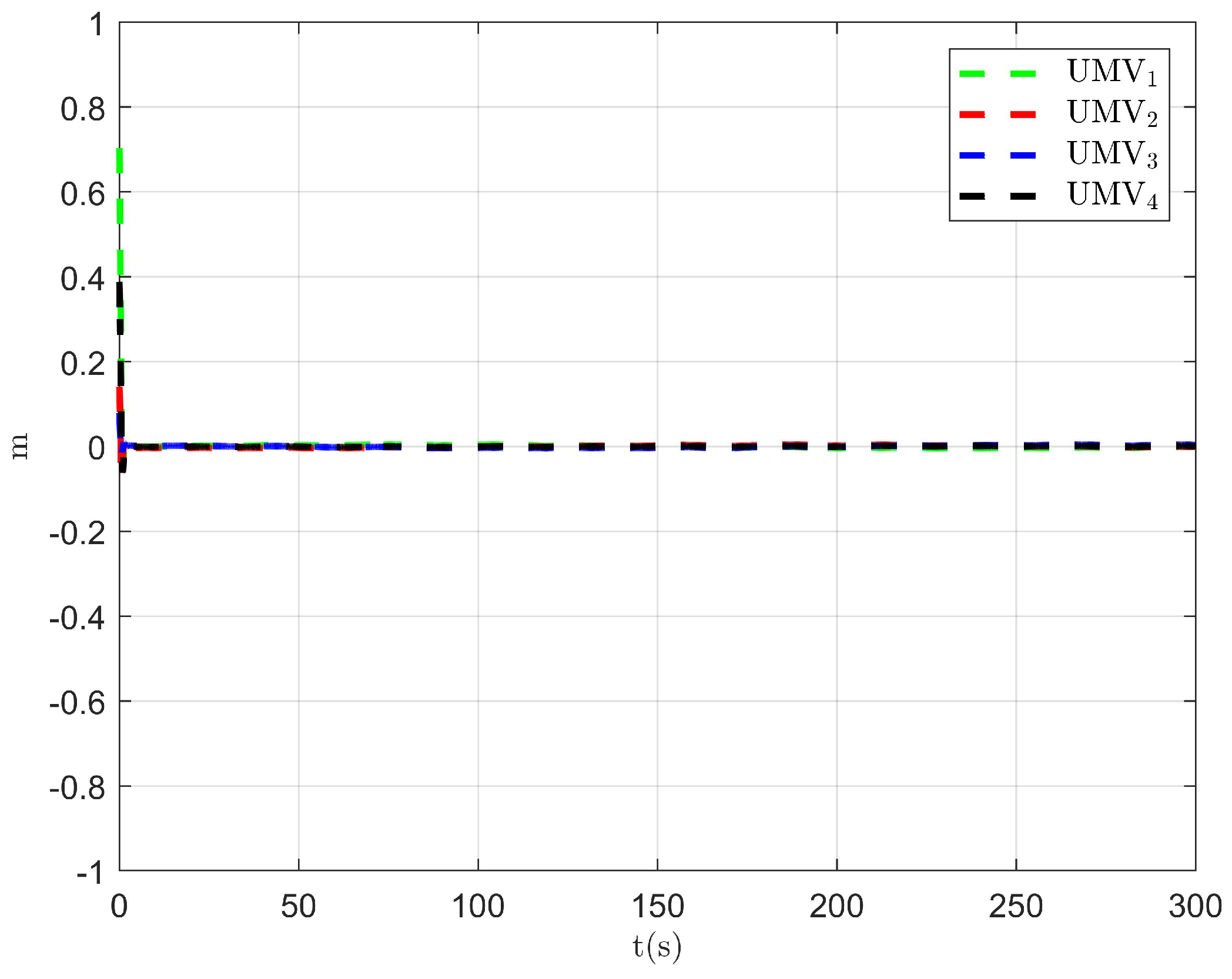
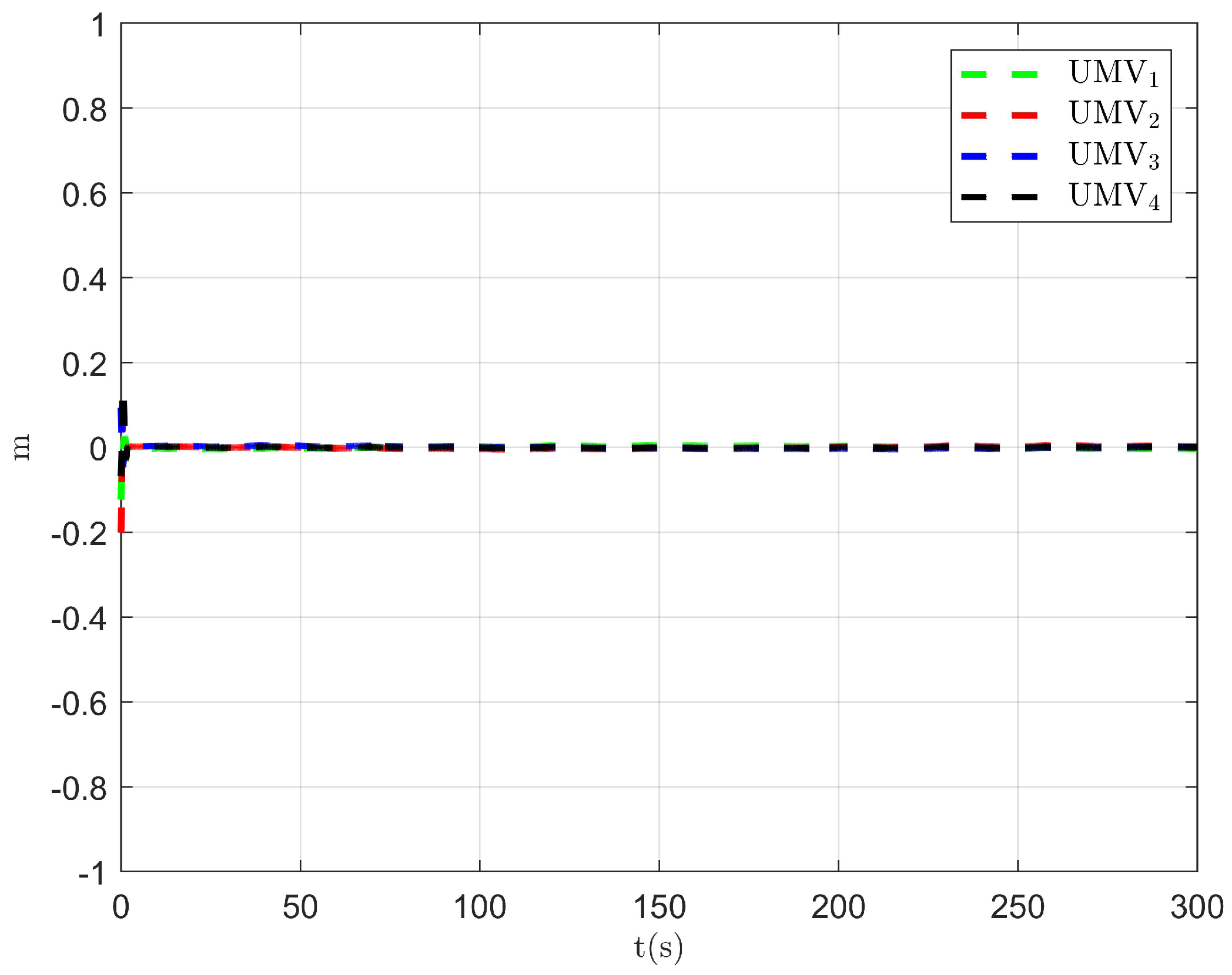
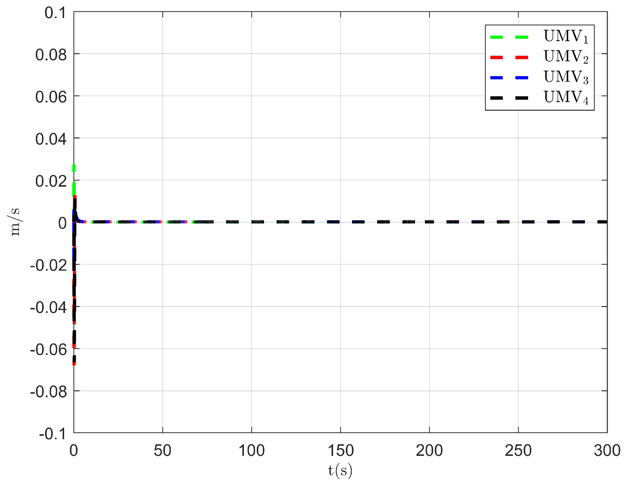
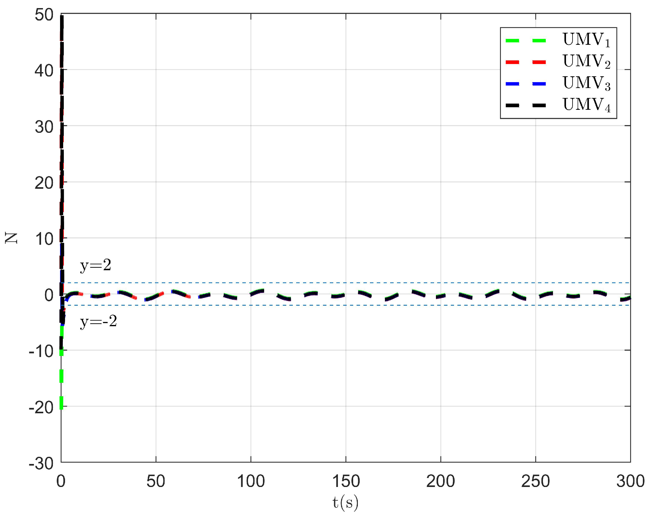
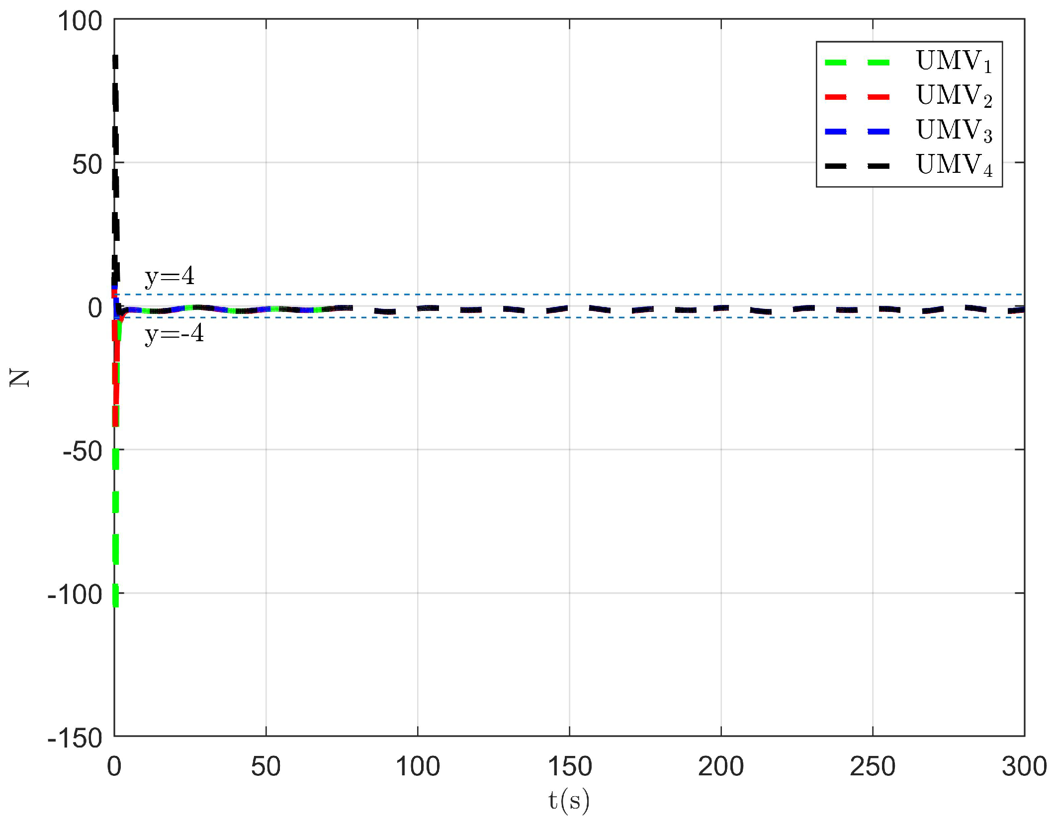
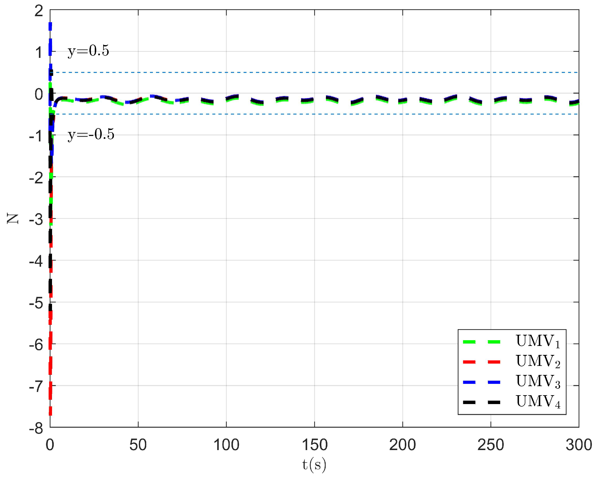
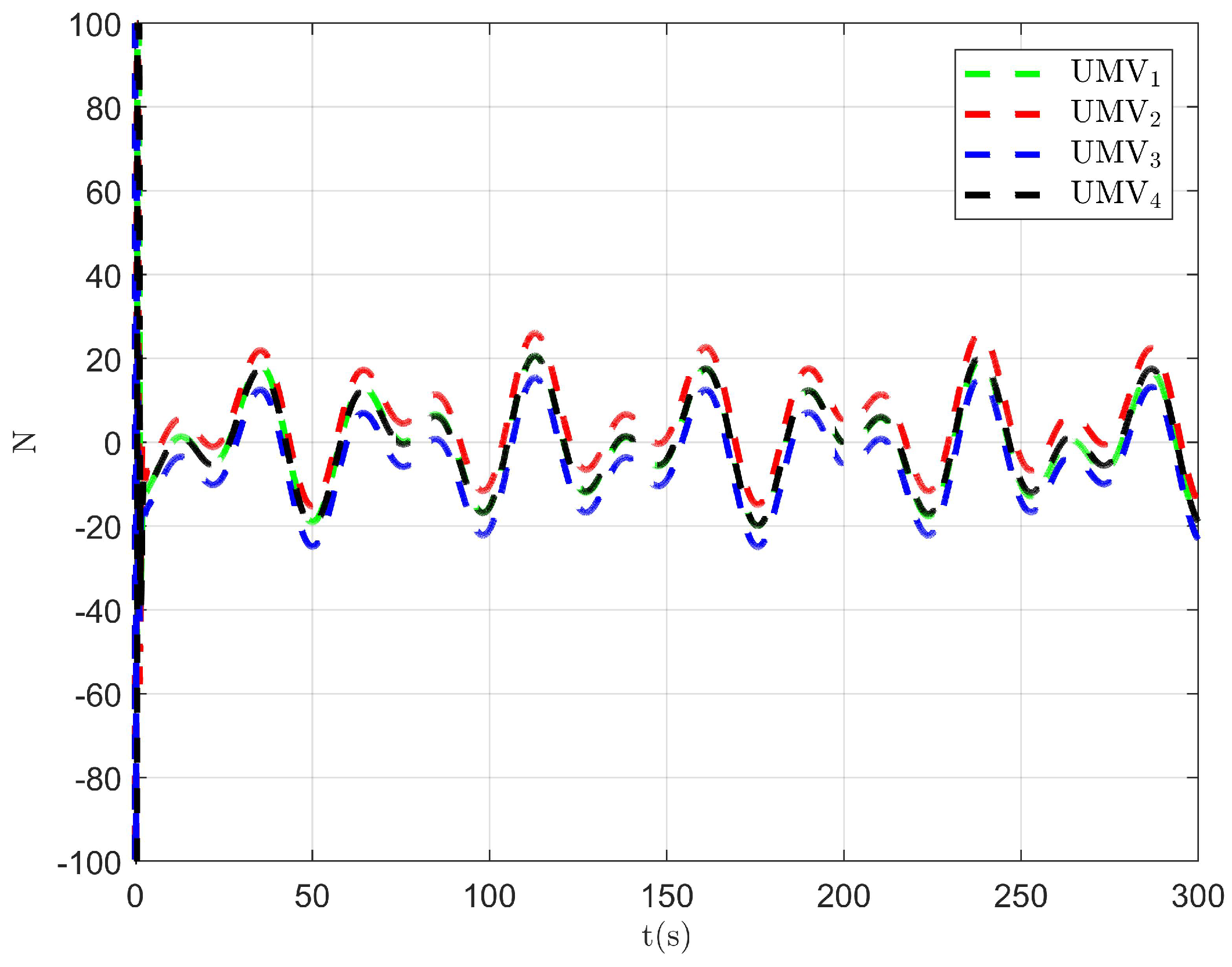
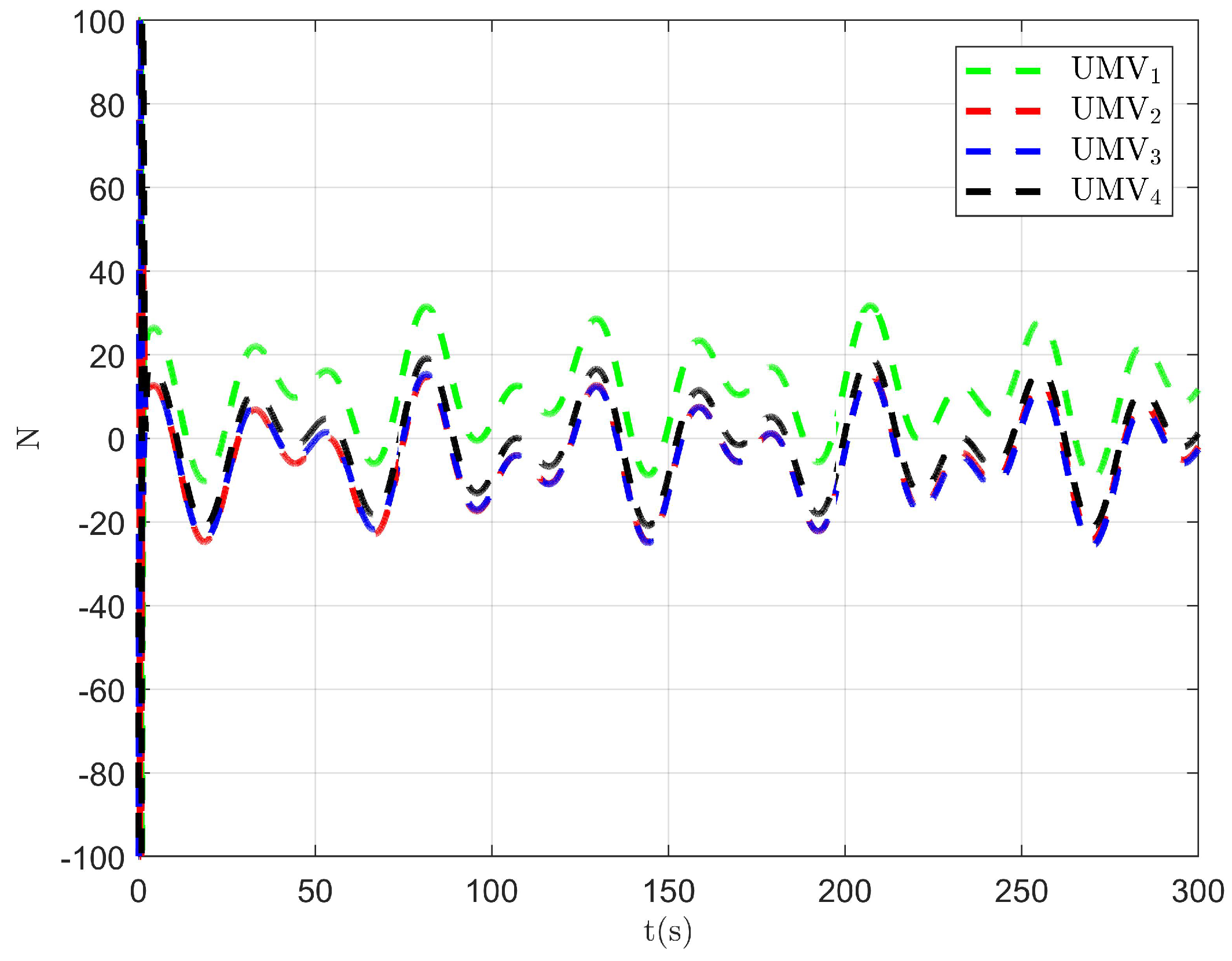
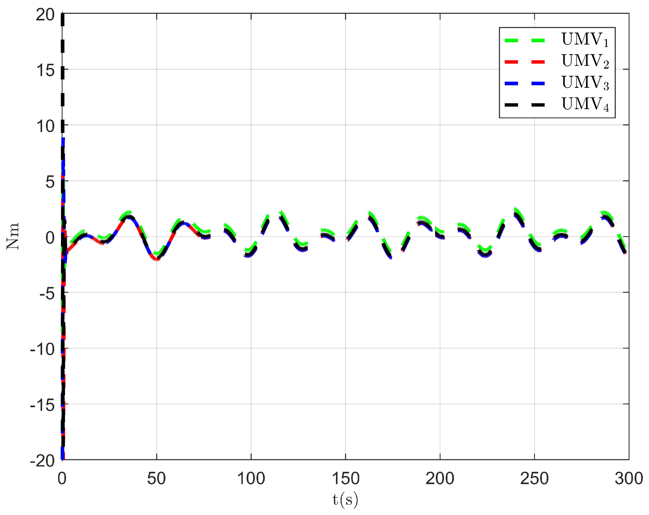
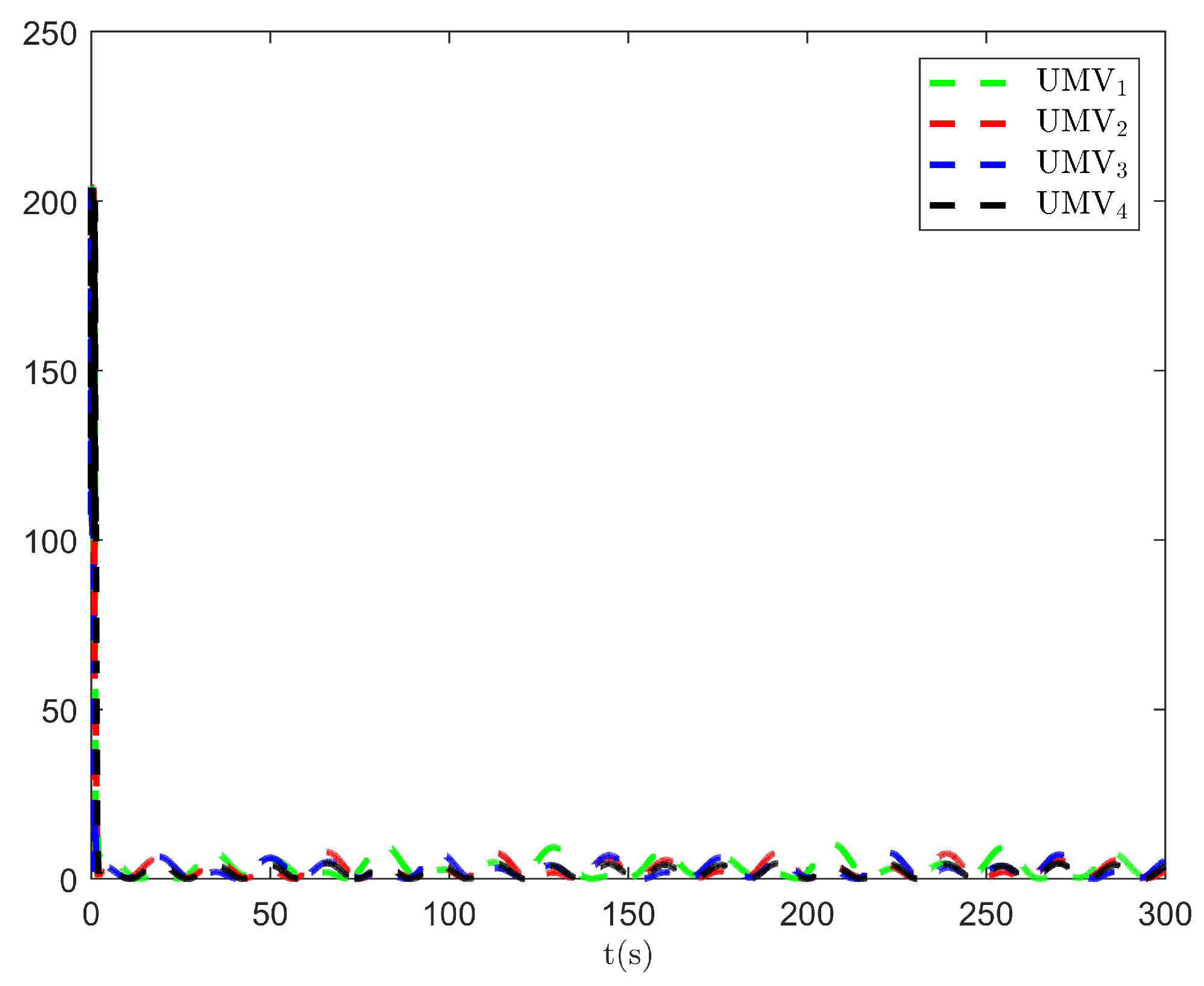
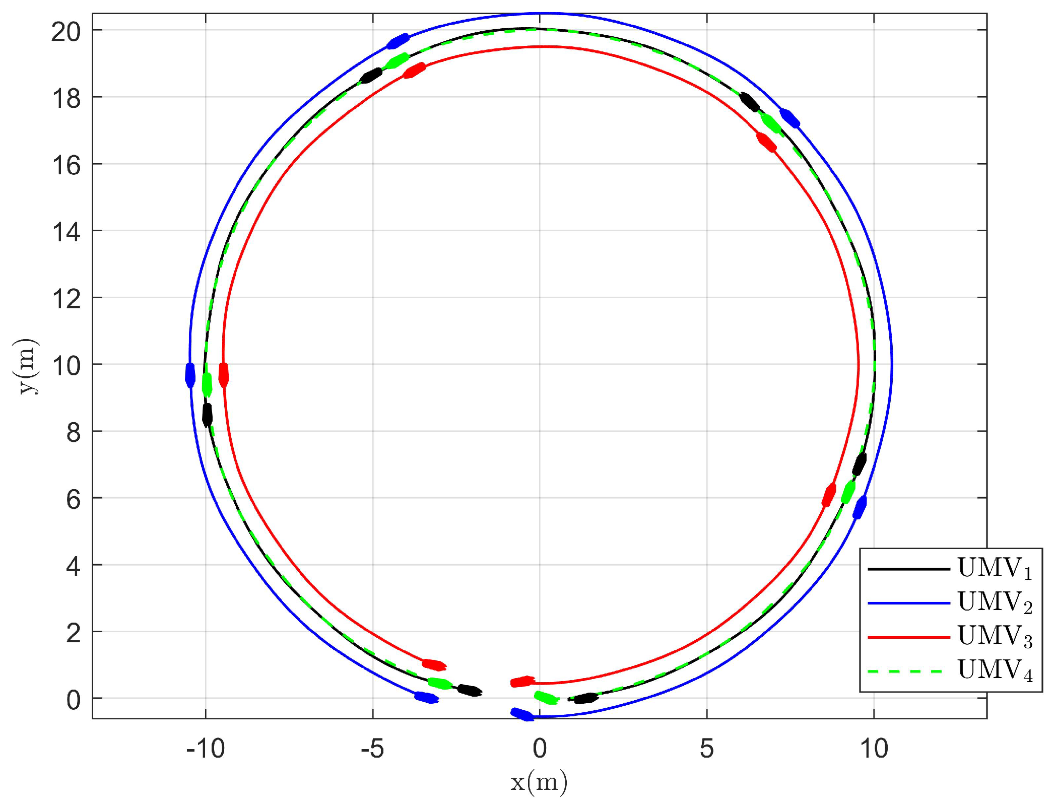
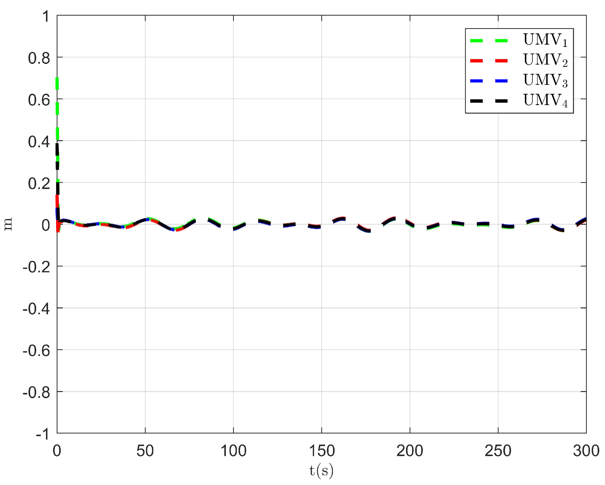
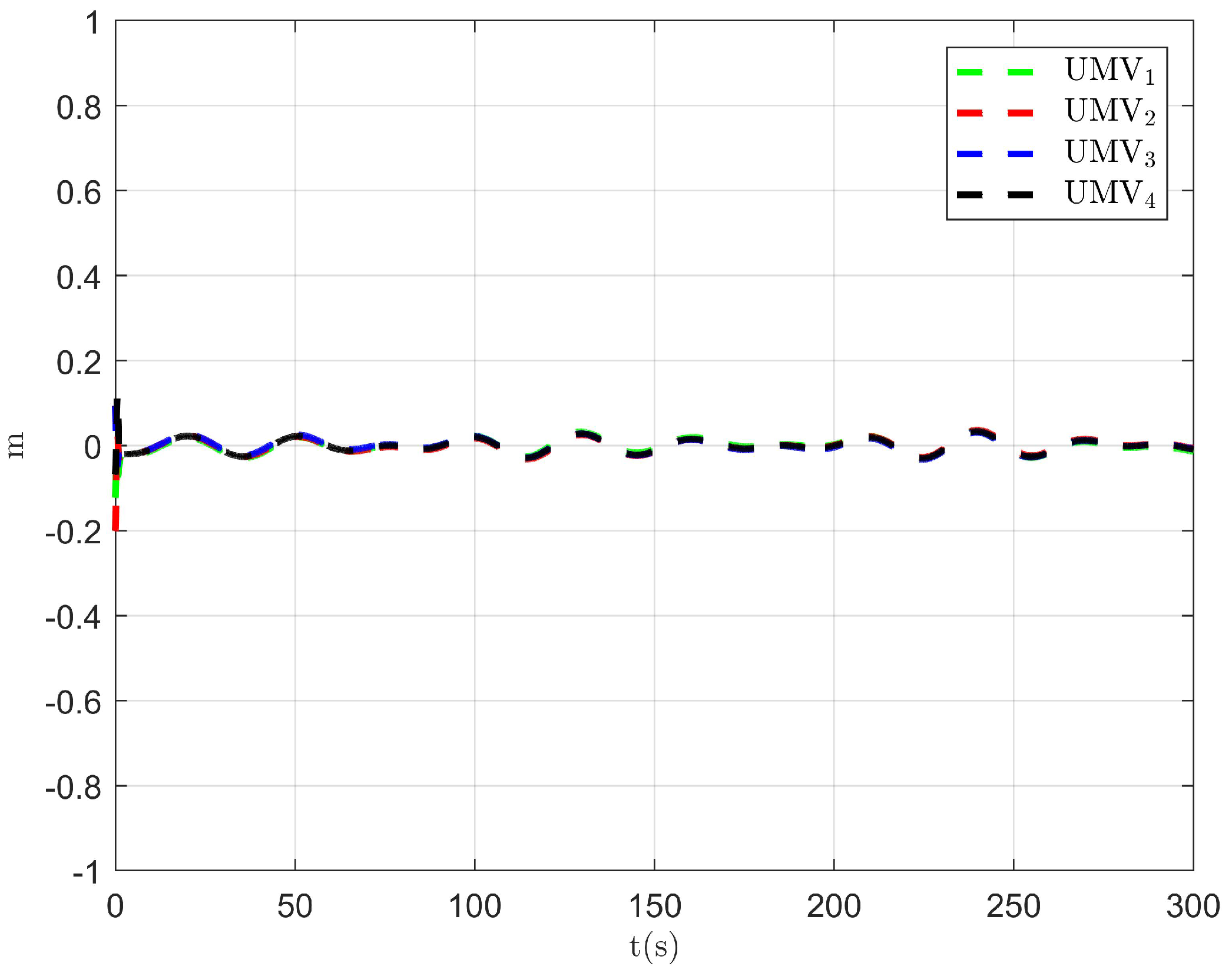
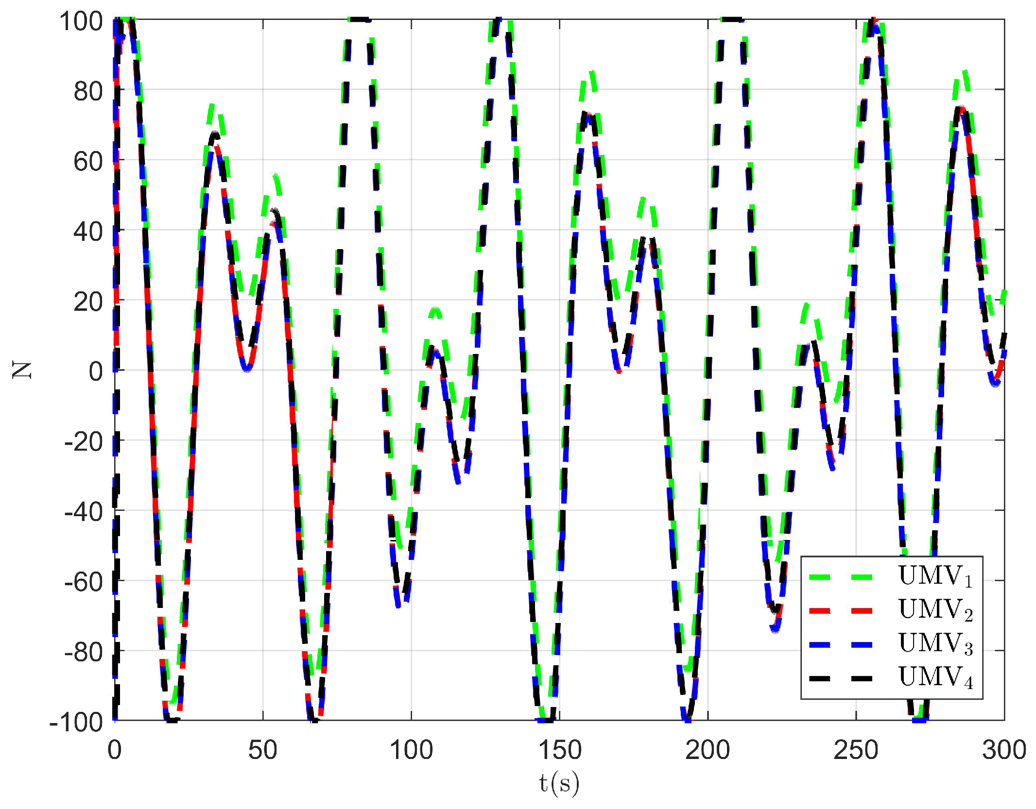
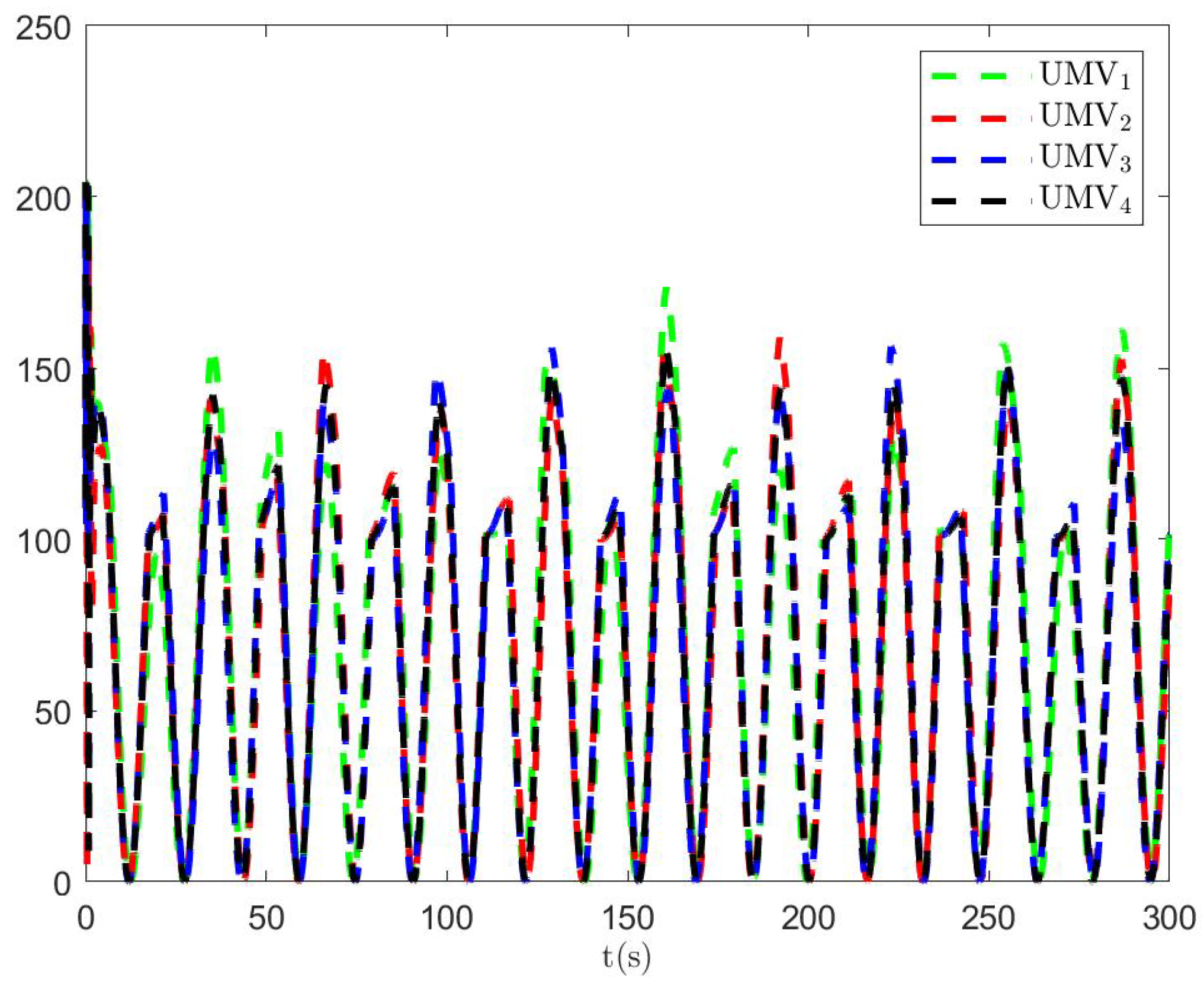
The simulation results are presented in Figure 2, Figure 3, Figure 4, Figure 5, Figure 6, Figure 7, Figure 8, Figure 9, Figure 10, Figure 11, Figure 12, Figure 13 and Figure 14. The tracking trajectory of the UMVs is shown in Figure 2, where it can be seen that the tracking control objective is achieved, and the UMVs maintain the desired formation. The tracking errors in the x and y directions are shown in Figure 3 and Figure 4, respectively. Initially, the errors are large due to the distance between the UMVs’ initial positions and the desired positions. However, once the UMVs approach the desired positions, the tracking errors tend to zero. Figure 5, Figure 6 and Figure 7 present the observer errors of the NSO. Since the initial value of the NSO is different from the actual value, the initial error is large. However, the designed updating law helps the NSO’s estimates converge to the true velocity values. The disturbance observer (DO) errors are shown in Figure 8, Figure 9 and Figure 10. As mentioned before, the applied disturbances , , and oscillate within the range of (−20, 20), (−20, 20), and (−2, 2), respectively. From Figure 8, Figure 9 and Figure 10, it can be observed that the DO errors stabilize within the range of [(−2, 2); (−4, 4); (−0.5, 0.5)], demonstrating that the designed DO effectively can reduce the impact of disturbances. The controller outputs are shown in Figure 11, Figure 12 and Figure 13, while the designed optimal index is shown in Figure 14. It can be seen that the proposed controller minimizes the optimal index.
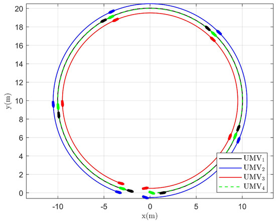
Figure 2.
Tracking trajectory of UMVs.
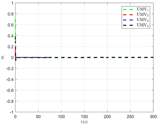
Figure 3.
Tracking error in the x-direction.
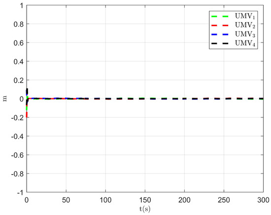
Figure 4.
Tracking error in the y-direction.
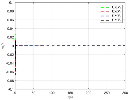
Figure 5.
Observer error of NSO .
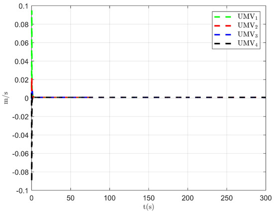
Figure 6.
Observer error of NSO .
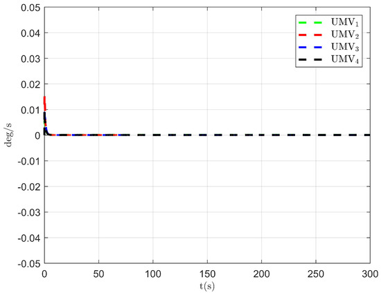
Figure 7.
Observer error of NSO .
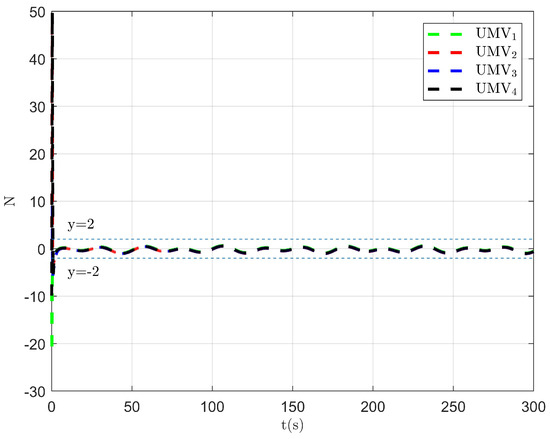
Figure 8.
Observer error of DO .
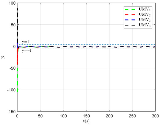
Figure 9.
Observer error of DO .
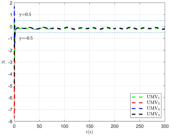
Figure 10.
Observer error of DO .
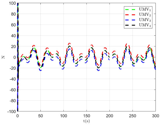
Figure 11.
Controller output .
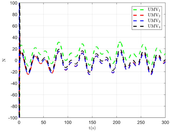
Figure 12.
Controller output .
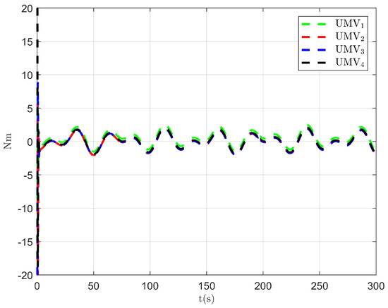
Figure 13.
Controller output .
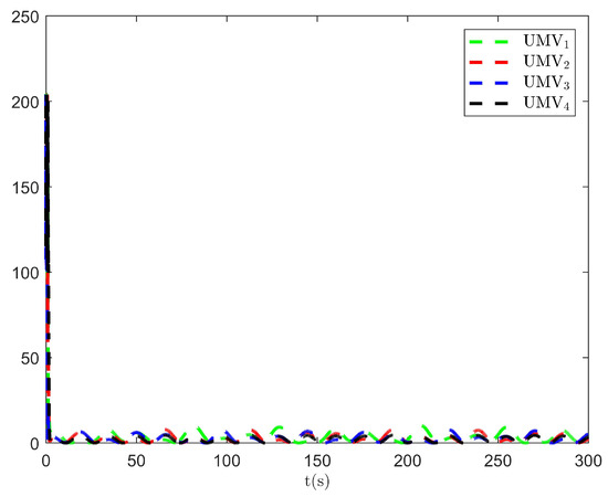
Figure 14.
Optimal index .
In conclusion, the simulation results demonstrate that the proposed optimal algorithm successfully handles the control task, and the NSO and DO can estimate the unmeasured velocities and unknown disturbances.
4.2. Comparison Study
To further demonstrate the disturbance rejection capability of the proposed algorithm, a comparative study is presented in this part. The controller adopted in this part is a fuzzy adaptive optimal controller without the disturbance rejection technique [34]. The experiment conditions, initial conditions, and applied disturbances are the same with the conditions given in Section 4.1.
The simulation results are presented in Figure 15, Figure 16, Figure 17, Figure 18, Figure 19, Figure 20 and Figure 21. As shown in Figure 15, the controller proposed in [34] achieves the tracking control objective. However, in Figure 16 and Figure 17, it is evident that the tracking errors are larger compared to Figure 3 and Figure 4. From Figure 18, Figure 19 and Figure 20, it can be observed that the controller output is larger compared to Figure 11, Figure 12 and Figure 13. This suggests that, under the applied disturbances, the lack of a disturbance rejection technique leads to larger tracking errors, which in turn requires a greater controller output to decrease tracking errors and achieve the control objective. This increased output results in a higher optimal index, as seen in Figure 21. Comparing Figure 21 to Figure 14, it becomes clear that the proposed controller achieves better performance in minimizing the optimal index. Therefore, the simulation results in Figure 15, Figure 16, Figure 17, Figure 18, Figure 19, Figure 20 and Figure 21 demonstrate that, under the disturbances , , and given in Section 4.1, the proposed control method with the DO demonstrates better control performance compared to the existing optimal control method without a disturbance rejection technique [34].
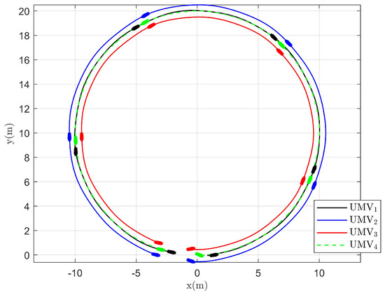
Figure 15.
Tracking trajectory of the existing control method [34].
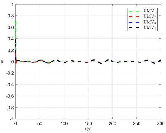
Figure 16.
Tracking error in the x direction of the existing control method [34].
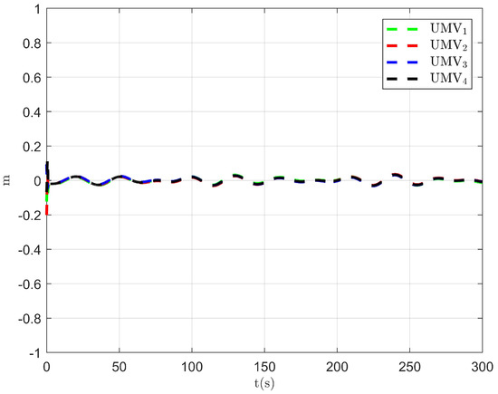
Figure 17.
Tracking error in the y direction of the existing control method [34].
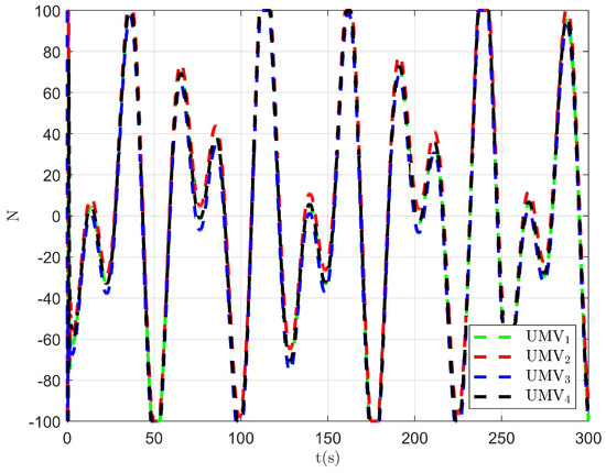
Figure 18.
Controller output of the existing control method [34].
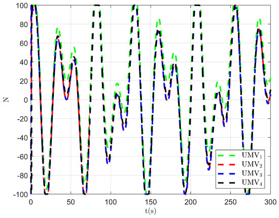
Figure 19.
Controller output of the existing control method [34].
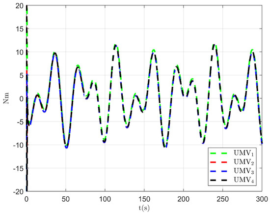
Figure 20.
Controller output of the existing control method [34].
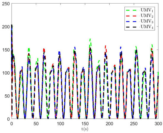
Figure 21.
Optimal index of the existing control method [34].
5. Conclusions
This paper has presented an observer-based adaptive optimal controller for tracking control problems of multiple UMVs with uncertain dynamics and unmeasured velocities. NSOs have been developed to manage the unmeasured velocities and the uncertain dynamics of the UMVs. An adaptive controller with an optimal compensation term has been implemented to achieve the control objective optimally. Additionally, a DO has been proposed to address unknown external disturbances. It has been proven that the proposed controller ensures all signals in the closed-loop system remain bounded. Simulation results have been provided to demonstrate the effectiveness of the proposed algorithm. From these results, it can be concluded that the proposed control algorithm has successfully achieved the control objectives and minimized the optimal index. The NSO and DO have effectively estimated the unmeasured velocities and unknown disturbances. To further illustrate the disturbance rejection capability of the proposed algorithm, a comparison study has been conducted using an existing method [34]. The simulation results of this comparison study have shown that, under the appied external disturbances, the proposed control algorithm can achieve better control performance by adopting the disturbance rejection technique.
Author Contributions
Methodology, L.-E.Y. and T.L.; software, L.-E.Y.; resources, Y.X. and T.L.; writing—original draft, L.-E.Y.; writing—review & editing, Y.X. and D.Z.; supervision, Y.X., T.L. and D.Z. All authors have read and agreed to the published version of the manuscript.
Funding
This work was partly supported by the National Natural Science Foundation of China under Grants 51939001, 52301418, 61751202, and 61976033, in part by Liaoning Revitalization Talents Program under Grant XLYC1908018. This work was also supported by the China Scholarship Council (Fund No. 202206570022).
Institutional Review Board Statement
Not applicable.
Informed Consent Statement
Not applicable.
Data Availability Statement
Data are contained within the article.
Conflicts of Interest
The authors declare no conflicts of interest.
References
- Peng, Z.; Wang, J.; Wang, D.; Han, Q.L. An Overview of Recent Advances in Coordinated Control of Multiple Autonomous Surface Vehicles. IEEE Trans. Ind. Inform. 2021, 17, 732–745. [Google Scholar] [CrossRef]
- Fossen, T.I. Marine Control Systems—Guidance, Navigation, and Control of Ships, Rigs and Underwater Vehicles; Marine Cybernetics: Trondheim, Norway, 2002. [Google Scholar]
- Peng, Z.; Liu, L.; Wang, J. Output-Feedback Flocking Control of Multiple Autonomous Surface Vehicles Based on Data-Driven Adaptive Extended State Observers. IEEE Trans. Cybern. 2021, 51, 4611–4622. [Google Scholar] [CrossRef] [PubMed]
- Peng, B.; Gu, N.; Wang, D.; Peng, Z. Model-Free Adaptive Disturbance Rejection Control of An RSV With Hardware-in-The-Loop Experiments. IEEE Trans. Ind. Electron. 2023, 70, 7507–7510. [Google Scholar] [CrossRef]
- Wu, W.; Peng, Z.; Wang, D.; Liu, L.; Han, Q.L. Network-Based Line-of-Sight Path Tracking of Underactuated Unmanned Surface Vehicles With Experiment Results. IEEE Trans. Cybern. 2022, 52, 10937–10947. [Google Scholar] [CrossRef] [PubMed]
- Peng, Z.; Wang, D.; Chen, Z.; Hu, X.; Lan, W. Adaptive Dynamic Surface Control for Formations of Autonomous Surface Vehicles With Uncertain Dynamics. IEEE Trans. Control Syst. Technol. 2013, 21, 513–520. [Google Scholar] [CrossRef]
- Gao, S.; Peng, Z.; Liu, L.; Wang, D.; Han, Q.L. Fixed-Time Resilient Edge-Triggered Estimation and Control of Surface Vehicles for Cooperative Target Tracking Under Attacks. IEEE Trans. Intell. Veh. 2023, 8, 547–556. [Google Scholar] [CrossRef]
- Peng, Z.; Wang, D.; Li, T.; Han, M. Output-Feedback Cooperative Formation Maneuvering of Autonomous Surface Vehicles With Connectivity Preservation and Collision Avoidance. IEEE Trans. Cybern. 2020, 50, 2527–2535. [Google Scholar] [CrossRef] [PubMed]
- Wang, F.; Zhang, H.; Liu, D. Adaptive Dynamic Programming: An Introduction. IEEE Comput. Intell. Mag. 2009, 4, 39–47. [Google Scholar] [CrossRef]
- Zhang, G.; Zhu, Q. Event-triggered optimal control for nonlinear stochastic systems via adaptive dynamic programming. Nonlinear Dyn. 2021, 105, 387–401. [Google Scholar] [CrossRef]
- Yuan, L.; Li, T.; Tong, S.; Xiao, Y.; Shan, Q. Broad Learning System Approximation-Based Adaptive Optimal Control for Unknown Discrete-Time Nonlinear Systems. IEEE Trans. Syst. Man Cybern. Syst. 2022, 52, 5028–5038. [Google Scholar] [CrossRef]
- Huang, Z.; Bai, W.; Li, T.; Long, Y.; Chen, C.P.; Liang, H.; Yang, H. Adaptive reinforcement learning optimal tracking control for strict-feedback nonlinear systems with prescribed performance. Inf. Sci. 2023, 621, 407–423. [Google Scholar] [CrossRef]
- Werbos, P.J. Approximate dynamic programming for realtime control and neural modelling. In Handbook of Intelligent Control: Neural, Fuzzy and Adaptive Approaches; Van Nostrand Reinhold: New York, NY, USA, 1992; pp. 493–525. [Google Scholar]
- Werbos, P.J. Consistency of HDP applied to a simple reinforcement learning problem. Neural Netw. 1990, 3, 179–189. [Google Scholar] [CrossRef]
- Jiang, Z.; Jiang, Y. Robust adaptive dynamic programming for linear and nonlinear systems: An overview. Eur. J. Control 2013, 19, 417–425. [Google Scholar] [CrossRef]
- Gao, X.; Long, Y.; Li, T.; Hu, X.; Chen, C.L.P.; Sun, F. Optimal Fuzzy Output Feedback Control for Dynamic Positioning of Vessels With Finite-Time Disturbance Rejection Under Thruster Saturations. IEEE Trans. Fuzzy Syst. 2023, 31, 3447–3458. [Google Scholar] [CrossRef]
- Wang, N.; Gao, Y.; Zhang, X. Data-driven performance-prescribed reinforcement learning control of an unmanned surface vehicle. IEEE Trans. Neural Netw. Learn. Syst. 2021, 32, 5456–5467. [Google Scholar] [CrossRef]
- Wang, N.; Gao, Y.; Zhao, H.; Ahn, C.K. Reinforcement Learning-Based Optimal Tracking Control of an Unknown Unmanned Surface Vehicle. IEEE Trans. Neural Netw. Learn. Syst. 2021, 32, 3034–3045. [Google Scholar] [CrossRef]
- Bellman, R.E. Dynamic Programming; Priceton Univ. Press: Priceton, NJ, USA, 1957. [Google Scholar]
- Peng, Z.; Wang, J.; Wang, D. Distributed Containment Maneuvering of Multiple Marine Vessels via Neurodynamics-Based Output Feedback. IEEE Trans. Ind. Electron. 2017, 64, 3831–3839. [Google Scholar] [CrossRef]
- Jiang, Y.; Peng, Z.; Wang, D.; Yin, Y.; Han, Q.L. Cooperative Target Enclosing of Ring-Networked Underactuated Autonomous Surface Vehicles Based on Data-Driven Fuzzy Predictors and Extended State Observers. IEEE Trans. Fuzzy Syst. 2022, 30, 2515–2528. [Google Scholar] [CrossRef]
- Deng, Y.; Zhang, X. Event-Triggered Composite Adaptive Fuzzy Output-Feedback Control for Path Following of Autonomous Surface Vessels. IEEE Trans. Fuzzy Syst. 2021, 29, 2701–2713. [Google Scholar] [CrossRef]
- Chen, W.H.; Yang, J.; Guo, L.; Li, S. Disturbance-Observer-Based Control and Related Method: An Overview. IEEE Trans. Ind. Electron. 2016, 63, 1083–1095. [Google Scholar] [CrossRef]
- Hu, X.; Wei, X.; Kao, Y.; Han, J. Robust Synchronization for Under-Actuated Vessels Based on Disturbance Observer. IEEE Trans. Intell. Transp. Syst. 2022, 23, 5470–5479. [Google Scholar] [CrossRef]
- Do, K. Practical control of underactuated ships. Ocean Eng. 2010, 37, 1111–1119. [Google Scholar] [CrossRef]
- von Ellenrieder, K.D. Dynamic surface control of trajectory tracking marine vehicles with actuator magnitude and rate limits. Automatica 2019, 105, 433–442. [Google Scholar] [CrossRef]
- Li, Z.; Sun, J.; Oh, S. Design, analysis and experimental validation of a robust nonlinear path following controller for marine surface vessels. Automatica 2009, 45, 1649–1658. [Google Scholar] [CrossRef]
- Gao, X.; Li, T.; Yuan, L.; Bai, W. Robust Fuzzy Adaptive Output Feedback Optimal Tracking Control for Dynamic Positioning of Marine Vessels with Unknown Disturbances and Uncertain Dynamics. Int. J. Fuzzy Syst. 2021. [Google Scholar] [CrossRef]
- Gao, X.; Bai, W.; Li, T.; Yuan, L.; Long, Y. Broad learning system-based adaptive optimal control design for dynamic positioning of marine vessels. Nonlinear Dyn. 2021, 105, 1593–1609. [Google Scholar] [CrossRef]
- Wondergem, M.; Lefeber, E.; Pettersen, K.Y.; Nijmeijer, H. Output Feedback Tracking of Ships. IEEE Trans. Control Syst. Technol. 2011, 19, 442–448. [Google Scholar] [CrossRef]
- Sarangapani, J. Neural Network Control of Nonlinear Discrete-Time Systems; CRC Press: Boca Raton, FL, USA, 2018. [Google Scholar]
- Vrabie, D.; Lewis, F. Neural network approach to continuous-time direct adaptive optimal control for partially unknown nonlinear systems. Neural Netw. 2009, 22, 237–246. [Google Scholar] [CrossRef]
- Skjetne, R.; Smogeli, Ø.; Fossen, T.I. Modeling, identification, and adaptive maneuvering of Cybership II: A complete design with experiments. IFAC Proc. Vol. 2004, 37, 203–208. [Google Scholar] [CrossRef]
- Sun, K.; Li, Y.; Tong, S. Fuzzy Adaptive Output Feedback Optimal Control Design for Strict-Feedback Nonlinear Systems. IEEE Trans. Syst. Man Cybern. Syst. 2017, 47, 33–44. [Google Scholar] [CrossRef]


Disclaimer/Publisher’s Note: The statements, opinions and data contained in all publications are solely those of the individual author(s) and contributor(s) and not of MDPI and/or the editor(s). MDPI and/or the editor(s) disclaim responsibility for any injury to people or property resulting from any ideas, methods, instructions or products referred to in the content. |
© 2024 by the authors. Licensee MDPI, Basel, Switzerland. This article is an open access article distributed under the terms and conditions of the Creative Commons Attribution (CC BY) license (https://creativecommons.org/licenses/by/4.0/).