Prediction-Based Submarine Cable-Tracking Strategy for Autonomous Underwater Vehicles with Side-Scan Sonar

Abstract

This study investigates the tracking of underwater cables using autonomous underwater vehicles (AUVs) equipped with side-scan sonar (SSS). AUV motion stability is crucial for effective SSS imaging, which is essential for continuous cable tracking. Traditional methods that derive AUV guidance rates directly from measured cable states often cause unnecessary jitter when imaging, complicating accurate detection. To address this, we propose a non-myopic receding-horizon optimization (RHO) strategy designed to maximize cable imaging quality while considering AUV maneuvering constraints. This strategy identifies the optimal heading decision sequence over a future horizon, ensuring stable and efficient cable tracking. We also employ a long short-term memory (LSTM) network to predict future cable states, further minimizing AUV motion instability during abrupt path changes. Given the computational limitations of AUVs, we have developed an efficient decision-making framework that can execute resource-intensive algorithms in real time. Finally, the robustness and effectiveness of the proposed algorithm were validated through comparative experiments. The results demonstrate that the proposed method outperforms existing methods in key metrics such as cable-tracking accuracy and AUV motion stability. This ensures that the AUV can acquire high-quality acoustic images of the submarine cable in an optimal state, enhancing the continuity and reliability of cable-tracking tasks.

1. Introduction

Submarine cables and pipelines are critical infrastructures for global communication and energy transmission; they are essential for international connectivity, energy security, and marine environmental protection [1]. Amid increasing globalization, submarine cables account for over 90% of global trans-oceanic communications while also interconnecting continental networks for power, oil, and gas transmission [2]. The structural integrity of these infrastructures is vital for the stability of global operations; however, they face numerous threats, including geological activities, extreme weather, anchor-chain dragging, and intentional sabotage [3,4]. Recent incidents of major oil spills and communication disruptions due to pipeline ruptures have highlighted the need for the routine monitoring and maintenance of submarine cables and pipelines [5].

Traditional inspection methods, which rely on survey vessels and remotely operated vehicles (ROVs), face significant limitations in deep-sea and large-area inspections [6]. Survey vessels, while equipped with sonar systems, face high operational costs, limited coverage, and inefficiencies in adverse conditions. ROVs, being constrained by umbilical cables, are limited in range and operational mobility, making them unsuitable for large-scale and long-distance tasks. With the growing complexity of the subsea network, these methods become increasingly labor-intensive and costly, especially in deep-sea environments.

Autonomous underwater vehicles (AUVs) provide a more efficient and flexible solution for inspecting submarine cables and pipelines [7]. Untethered from umbilical cables, AUVs can autonomously perform long-duration inspections over large areas, making them particularly advantageous in deep-sea environments, complex terrains, and large-scale operations. With advanced sensors and autonomous navigation systems, AUVs dynamically adjust their path in real time, ensuring operational continuity and higher efficiency. Compared to ROVs, AUVs significantly reduce operational complexity and costs, making them a leading technology for subsea infrastructure inspection.

In AUV-based inspection missions, sensor selection plays a crucial role in ensuring the effectiveness of the operation. Commonly used sensors include optical, magnetic, and acoustic sensors [6]. Optical sensors, such as cameras, deliver high-resolution images but are constrained by water turbidity and lighting conditions, making them suitable primarily for shallow water or short-range inspections [8]. Magnetic sensors, which identify cables by detecting changes in the electromagnetic field, are effective for short-range localization; however, their limited range and sensitivity to environmental interference reduce their effectiveness in large-scale operations [9]. Acoustic sensors, particularly side-scan sonar (SSS), offer a superior detection range and are less affected by environmental factors such as water turbidity. SSS generates high-resolution, two-dimensional seabed imagery by transmitting acoustic waves and processing the echo signals [10]. This enables precise visualization of the cable and its surrounding environment, making it particularly suitable for complex and large-scale detection tasks.

The remainder of this paper is organized as follows: Section 2 reviews related works; Section 3 outlines the framework and problem formulation for cable tracking using side-scan sonar; Section 4 details the proposed cable tracking methodology; Section 5 discusses algorithm validation; and Section 6 offers additional insights.

2. Related Work

The traditional preset waypoint method ensures that the AUV moves in a straight line and obtains clear SSS images. However, this method is inefficient and often leads to cables disappearing from the field of view (FOV) of onboard sensors due to deviations in cable-laying paths and accumulated navigation errors. Consequently, AUVs must adjust their heading online based on measurement data to adapt to changes in the cable’s status [11].

Various strategies have been proposed to address these challenges. The line-of-sight (LOS) method is one of the most widely adopted control strategies for subsea cable tracking. The LOS algorithm emulates the behavior of a helmsman, guiding the AUV toward a look-ahead point along the projected path of the cable. Upon detecting a cable, the AUVs realize cable tracking by adjusting their vertical rudder angles or the port and starboard thrust [12]. In Ref. [13], the cable-tracking task was framed as a path-tracking problem in the horizontal plane, modeling the cable with a uniform motion model and developing an adaptive LOS guidance algorithm suitable for side-scan sonar (SSS). In Ref. [9], a vector field-based guidance method was proposed to tackle the cable-tracking problem for use with underactuated AUVs without a tracking error dynamics model, incorporating new noise-resistant techniques to reduce the effects of noise on the system. Ref. [14] introduced an advanced reinforcement learning control system to address the action selection problem of AUVs during cable tracking. In Ref. [15], the intersections between the cable and image boundaries in sonar images were identified as AUV tracking targets, leading the authors to transform the cable-tracking problem into a series of point-tracking tasks. In Ref. [16], the authors achieved cable tracking by eliminating the relative directions and distances between the AUVs and cables. Similarly, Ref. [17] proposed two motion control objectives: maintaining the cable vertically in the image and centering the cable in the frame, using deviation as the controller input. The authors of [18] introduced a novel cable-tracking method by reformulating the tracking problem as a target interception issue, generating reference headings with proportional navigation guidance laws and employing model predictive control (MPC) for tracking.

Existing control strategies map the real-time cable state to the AUV’s motion. Aggressive guidance laws can lead to jittery control inputs, negatively impacting cable imaging and detection. Conversely, overly conservative guidance laws may cause AUVs to respond sluggishly to changes in cable status, resulting in them disappearing from the SSS field of view. Non-myopic methods enable AUVs to track underwater targets more smoothly. The authors of [19] reformulated the seabed terrain-following control (STFC) problem as a trajectory prediction and tracking issue. They employed a long short-term memory (LSTM) network to forecast future seabed terrain and used nonlinear model predictive control to enable AUVs to maintain an appropriate height above the seabed. In Ref. [20], a unified receding horizon optimization (RHO) scheme was proposed, addressing sensor myopia constraints and transforming the path-planning problem into an RHO problem based on a spline path template. For the underwater dynamic target-tracking challenge, Ref. [21] predicted target trajectories using a time-gain Elman neural network and applied model predictive control for tracking. The Centre for Maritime Research and Experimentation (CMRE) introduced a data-driven approach to enhance target-tracking performance in AUV multi-static surveillance scenarios, aiming to minimize the estimation error when calculating the target position using an onboard processor [22].

There is a dearth of research on non-myopic methods for solving submarine cable-tracking problems. Existing studies have focused primarily on accurately extracting cables from noisy sonar images, rather than on controlling the AUV motion to obtain clearer sonar images. Research efforts aimed at improving the SSS imaging performance are mainly concentrated on underwater target search tasks. The authors of [23] extended the information gain method for adaptive path planning in SSS-equipped AUVs, adjusting navigation states based on measurements to ensure optimal imaging quality during coverage observations. Ref. [24] proposed an adaptive strategy for sonar-based AUV data collection to minimize target occlusion caused by seabed ripples during the imaging process. Ref. [25] proposed a novel coverage path-planning method that considered the target existence probability and SSS detection capability to reduce image distortion in underwater search and rescue missions.

In summary, numerous studies have examined the factors affecting SSS imaging and applied theoretical findings to seabed target searches. However, no research specifically addresses the stable imaging problem for tracking targets like seabed cables. This paper proposes a non-myopic method to tackle the SSS-based submarine cable stable tracking problem by identifying the optimal heading-decision sequence for AUVs. The optimization criteria focus on maximizing cable tracking accuracy, ensuring AUV motion stability, and maintaining high-quality SSS imaging. Our approach balances these metrics by optimizing parameters such as heading control and motion smoothness for optimal tracking performance. We have introduced a time series concept to develop a trajectory prediction model based on an LSTM network for forecasting future cable trends. Additionally, a simplified decision-making method is proposed to reduce the algorithm’s computational burden. Finally, the robustness and effectiveness of the proposed algorithm are validated through comparative experiments, demonstrating that our method outperforms existing approaches in terms of key performance metrics, including cable tracking accuracy and AUV motion stability.

The contributions of this study can be summarized as follows:

(1)

Applying the non-myopic method to the submarine cable tracking task, we optimize the AUV’s heading by combining the characteristics of SSS measurements. This ensures high-quality imaging of the side-scan sonar while achieving stable tracking of the cable.

(2)

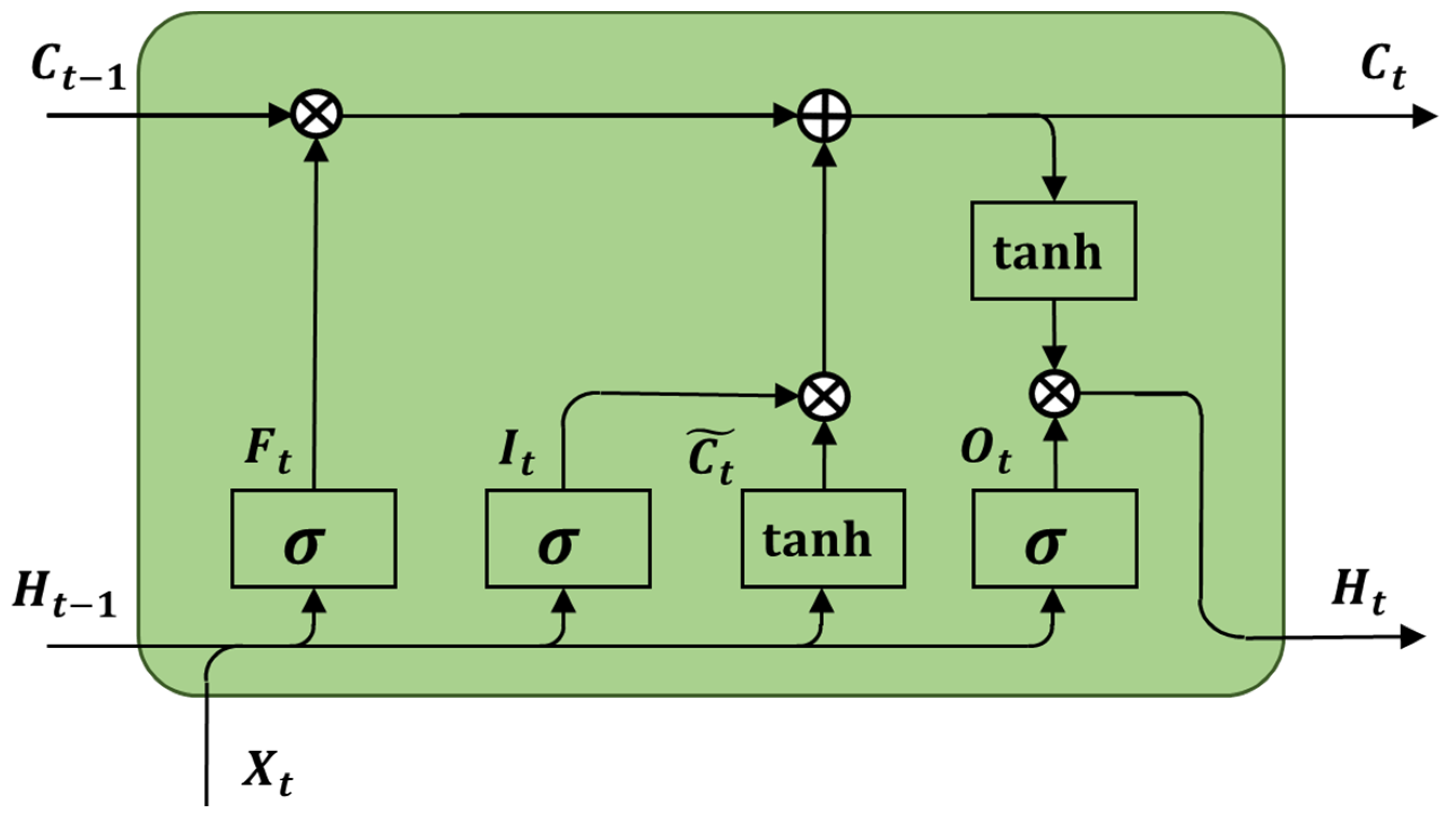
The measured sequence of cable states is viewed as a set of time series arranged at equal time intervals, utilizing LSTM networks to predict future cable trends, thereby mitigating the negative impact of the myopia of onboard sensors.

3. Preliminaries

Offshore wind power is transmitted via cables to onshore distribution stations to provide electricity to communities. SSS-equipped AUVs can acquire acoustic images of cables and the surrounding environment, providing crucial support for cable servicing and maintenance, as shown in Figure 1.

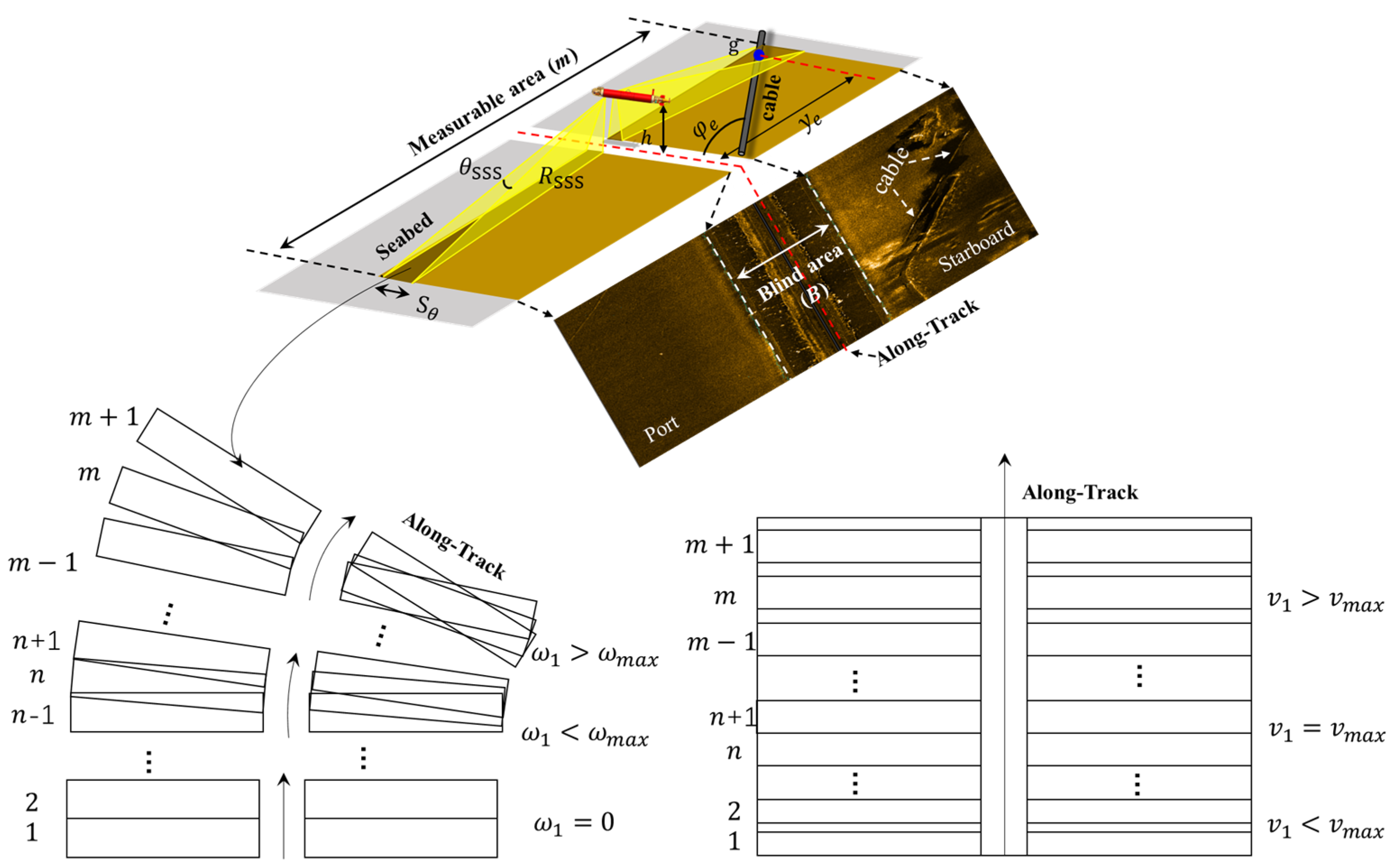
3.1. Introduction to Side-Scan Sonar Imaging

SSS uses acoustic reflection signals from fan-shaped pulses that are transmitted to the seafloor to generate images. The signal intensity represents targets that are made from different materials [26]. As the AUV moves forward in a straight line, the onboard SSS collects data and leaves a narrow, unscanned corridor. The SSS echoes are combined with the onboard navigation data to provide a georeferenced mosaic of the seabed, as shown in Figure 2 [27]. Here, h denotes the AUV’s height from the seabed, m denotes the coverage area of the SSS, B denotes the blind area, the blue dot g(x,y,φ) denotes the midpoint of the cable in the sonar image, (x,y) denotes the cable position, φ denotes the azimuth angle, φ_e denotes the angle between the cable and AUV, and y_e denotes the horizontal distance. As shown in Figure 2, the excessive turning velocity of the SSS (${\omega }_1>{\omega }_{max}$) creates blind spots on the port side and a redundant overlap on the starboard side. Similarly, high forward velocity ($v_1>v_{max}$) leads to discontinuities between adjacent sonar beams.

Factors affecting the SSS’s performance can be categorized into four classes [24]: target characteristics (TCs), underwater environment (UE), SSS parameters (SPs), and AUV status (AS). Based on previous survey data, we identified several key challenges in tracking cables using SSS, even when the cables are laid flat on a smooth seabed without burial or suspension (Figure 3):

(1)

During any sharp turns of the sonar device, any areas outside the turn were completely missed owing to the finite ping rate of the SSS, while areas within the turn could be heavily distorted. In both cases, identifying targets in the images could be challenging [28];

(2)

The relative angle between the sonar beam and the underwater cable was a crucial factor influencing target imaging. When the SSS moved parallel to the cable, the strongest acoustic echoes could be obtained because of specular reflection [29];

(3)

The probability of detecting a target within the lateral range of the sonar tracking was a function of the distance (a), and the image quality tended to degrade considerably over long distances [23,30,31].

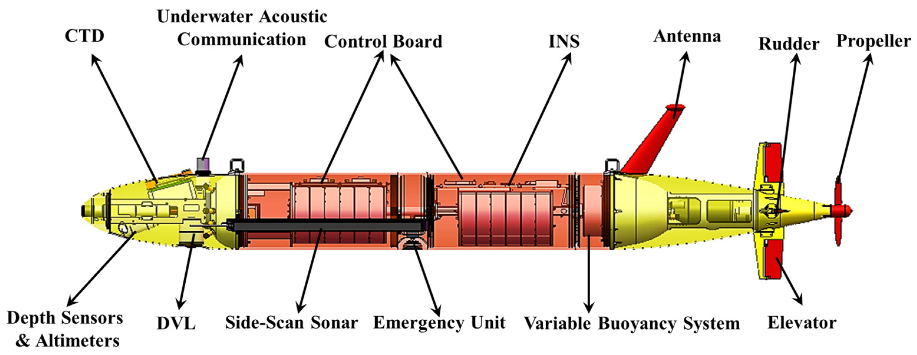
3.2. “Sea Whale” AUV

The “Sea Whale” AUV is a hybrid, lightweight, long-range underwater vehicle capable of performing marine environment observations and undersea target detection at depths of up to 1000 m [32,33,34]. It is approximately 3.3 m in length, with a diameter of 0.35 m, and its system composition is shown in Figure 4. The SSS is mounted on the front section of the AUV, allowing it to collect real-time environmental images and conduct image data processing and target detection [35]. The “Sea Whale” AUV adopts a dual-mode control system comprising a mission planning board (MPB) and flight control board (FCB). The MPB processes the sensor data and runs intelligent algorithms, providing control instructions for the FCB, including navigation height, heading, and speed [36].

The AUV can achieve stable cable tracking by adjusting its heading in real time. When moving in the horizontal plane, the effects of heave, roll, and pitch motion parameters can be neglected. The equations of motion can be expressed as follows:

$$\left\{\begin{array}{c}\dot{x}=u\mathit{cos}\psi -v\mathit{sin}\psi \approx u_0\mathit{cos}\psi \\ \dot{y}=u\mathit{sin}\psi +v\mathit{cos}\psi \approx u_0\mathit{sin}\psi \\ \dot{\psi }=r\end{array}\right.,$$

(1)

where [x,y,ψ]^T denotes the position and direction, [u,v,r] denotes the surge, sway, and yaw, respectively, and u₀ denotes the resultant tangential velocity of the vehicle.

3.3. Problem Statement

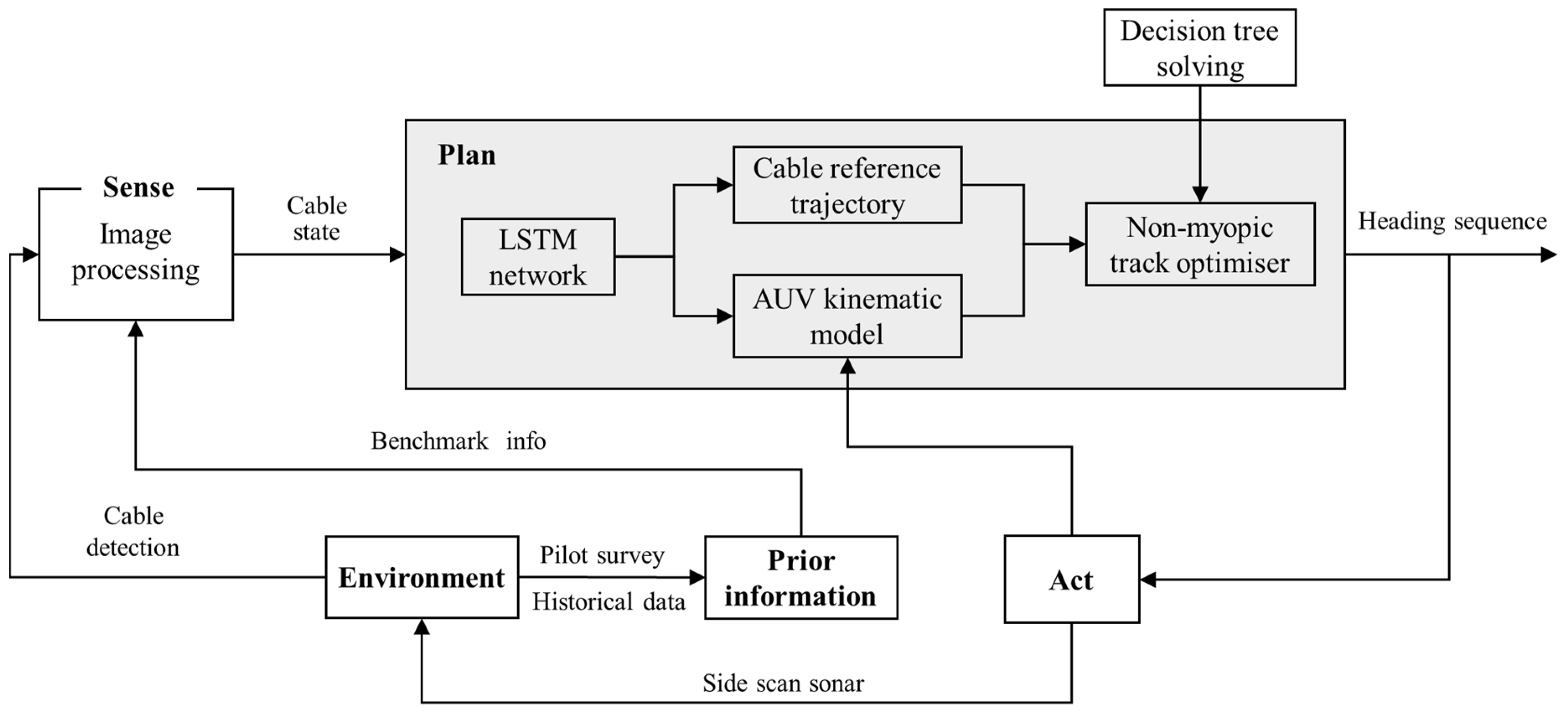
When the AUV tracks the cable, its workspace is constrained by the measurement range of the SSS, such as the curves of c₁(x) and c₂(x) shown in Figure 5. Specifically, the non-myopic method establishes a relationship between the AUV’s inputs (heading decisions) and outputs (the path’s stable quality) by predicting the state over multiple future steps. To achieve high-quality measurements, the following three problems need to be solved:

Problem 1.

Cable state prediction: Based on the measured cable history data $X={\left[x_1,x_2,\dots ,x_{N_h}\right]}^T$, predict the future state$\widehat{X}={\left[{\widehat{x}}_1,{\widehat{x}}_2,\dots ,{\widehat{x}}_{N_p}\right]}^T$, where N_h denotes the volume of historical data and N_p denotes the number of next steps to be predicted.

Problem 2.

AUV heading optimization: The predicted cable state information  $\widehat{X}$ and AUV kinematic model can be combined to optimally solve the AUV optimal heading sequence ${\psi }_{opt}=[\mathsf{\Delta }{\psi }_1,\mathsf{\Delta }{\psi }_2,\cdots ,\mathsf{\Delta }{\psi }_{N_P}]$.

Problem 3.

Decision sequence pruning and optimization: Optimizing pruned decision trees for computationally underpowered embedded systems.

Comparative experiments were conducted, combined with practical engineering applications, to verify the effectiveness of the proposed method, thereby offering crucial technical guidance for the future automated inspection of submarine cables.

4. Methodology

The tracking system framework described here follows the Sense → Plan → Act closed-loop structure, as shown in Figure 6. During the sensing phase, the cable features are extracted from the sonar image. During the planning phase, the LSTM network is first used to predict future cable trends based on the historical data sequences. Subsequently, a non-myopic receding-horizon strategy can be employed to search for the optimal sequence of headings for potential future AUV maneuvers. Finally, the decision tree is pruned to enable the algorithm to run in real time on embedded systems.

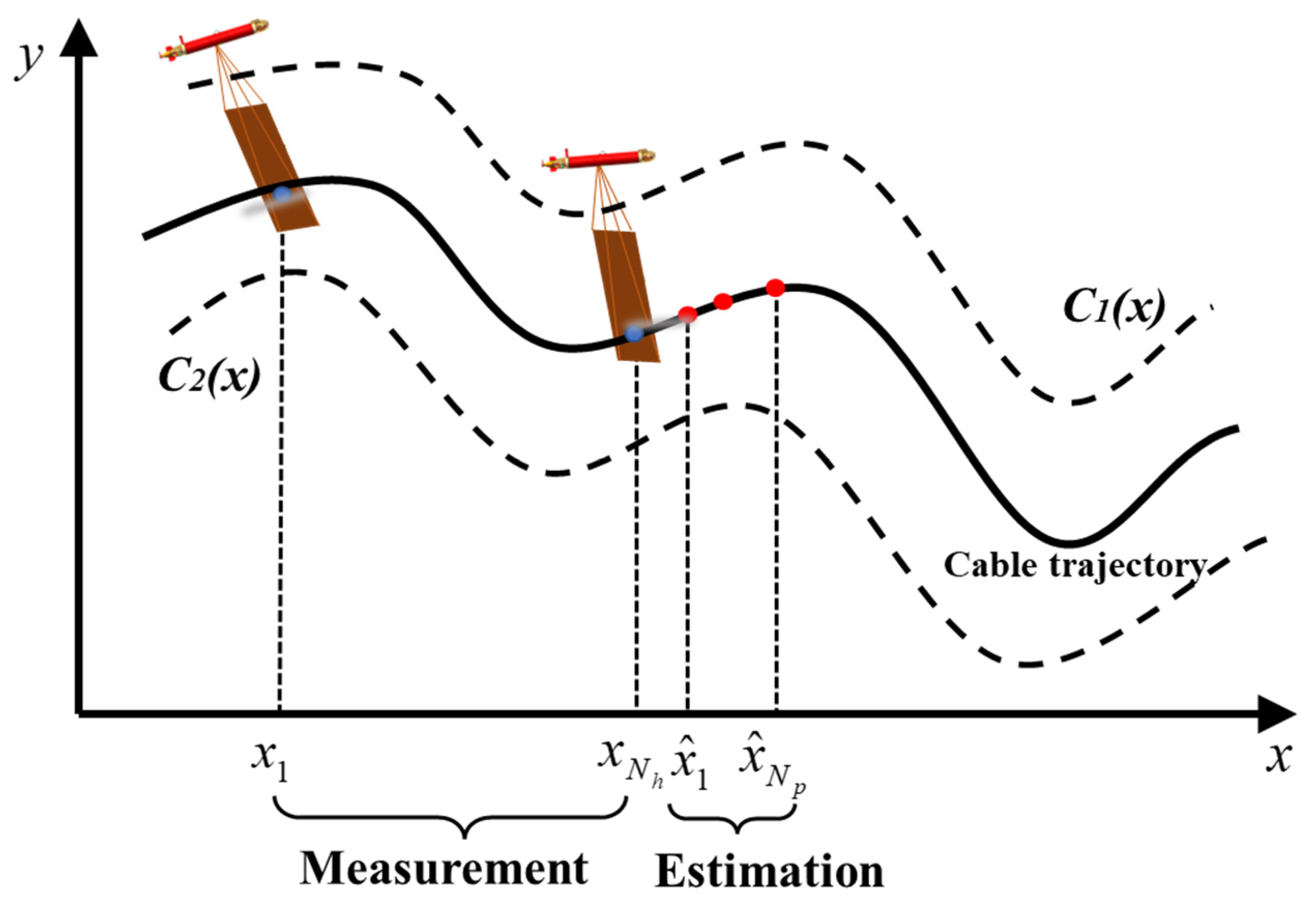
4.1. Cable State Prediction

Given that a cable is an artificial object on the seafloor with inherent continuity, its trajectory can be viewed as the motion path of a mass point subject to specific kinematic constraints [13]. When tracking a cable using an AUV equipped with SSS, the measured state sequence of the cable can be viewed as a set of time sequences $S=[s_0,s_1,\cdots ,s_k,\cdots ,s_N]$, where N denotes the length of the sequence. $s_k=\left(x_k,y_k,{\phi }_k\right)$ represents the position and angle of the cable measured at moment k, also serving as an input. In S, the nonlinear mapping relationship between S_k and its preceding n data $s_{k-1},s_{k-2},\cdots ,s_{k-n}$ can be represented by the nonlinear mapping function $G(\cdot )$, as follows:

$$s_k=G\left(s_{k-1},s_{k-2},\cdots ,s_{k-n}\right).$$

(2)

The LSTM network is a variant of a recurrent neural network (RNN) specializing in processing sequence data and is more suitable for solving time-series prediction problems owing to certain memory effects [37]; it has been successfully applied in underwater terrain prediction [38] and ocean feature forecasting [19]. The LSTM network adds three logical control units—that is, the input, output, and forget gates—to the basic structure of the RNN. The specific architecture is shown in Figure 7.

The memory units record the cell state from the previous time step using self-recurrent connections. The inputs consist of the input vector (X_t) and the output of the hidden state of the previous layer (H_t−1), where the output represents the candidate cell state ${\tilde{C}}_t$, which can be expressed as follows:

$${\tilde{C}}_t=\mathit{tan}h(X_t{W}_{xc}+H_{t-1}{W}_{hc}+b_c).$$

(3)

The input gate controls the input activation flow in the memory unit. The two inputs are X_t and H_t−1, and the output is the input-gate state I_t, which can be expressed as follows:

$$I_t=\sigma (X_t{W}_{xi}+H_{t-1}{W}_{hi}+b_i)$$

(4)

$$C_t=F_t\otimes C_{t-1}+I_t\otimes {\tilde{C}}_t.$$

(5)

The forget gates control the state of the memory unit so that it can adaptively forget or reset the cell state. The two inputs are X_t and H_t−1, and the output is the forget-gate state (F_t), which can be expressed as follows:

$$F_t=\sigma (X_t{W}_{xf}+H_{t-1}{W}_{hf}+b_f).$$

(6)

The output gate controls the output activation flow into the LSTM cell output. The two inputs are X_t and H_t−1, and the output is the output-gate state (O_t), which can be expressed as follows:

$$O_t=\sigma (X_t{W}_{xo}+H_{t-1}{W}_{ho}+b_o)$$

(7)

$$H_t=O_t\otimes \mathit{tan}h(C_t)$$

(8)

where b_β denotes the deviation, W_αβ denotes the weight between α = {x, h} and β = {c, f, i, o}, and σ denotes the sigmoid function.

To facilitate data input and prediction, this study designs a sliding window, as shown in Figure 8, selecting s₁:s_t as the first set of input data, with the output data being s_t+1, then selecting s₂:s_t+1 as the second set of input data, with the output data being s_t+2, and so on. To recursively realize the prediction of the future N_p step cable state, the prediction expression can be expressed as shown in the figure, where t denotes the size of the sliding window.

4.2. Cable-Tracking Method Based on Receding-Horizon Strategy

4.2.1. Construct Cost Function Based on SSS Characteristics

We treat the submarine cable-tracking problem as an SSS-based trajectory tracking challenge, integrating a receding-horizon algorithm with a finite forward-looking control scheme to achieve stable tracking by incorporating its impact on the cost function of future actions. The heading is the sole control variable for cable tracking. This section focuses on designing an optimal heading-selection strategy for the AUV, considering the scenario’s evolution over a future time window to balance different objectives. For a specific cable-tracking task—that is, one with fixed TCs, UE, and SPs—three guidelines can be defined, as follows:

(1)

A smaller turning angle avoids distortion of the sonar image;

(2)

Imaging is best when the cable and AUV are parallel; and

(3)

The cable is kept at a certain distance from the AUV, to locate it in the middle of the sonar image.

The first objective function (f₁) denotes the constraint of the AUV heading change, which should be avoided as much as possible while the AUV tracks the cable—that is, fewer turns can reduce aberrations in the sonar image.

$$f_1\left(\psi \right)={\sum }_{i=1}^{N_p}\left({\alpha }_{i-1}\left|{\psi }_i-{\psi }_{i-1}\right|\right),$$

(9)

Here, $\psi =[{\psi }_1,{\psi }_2,\cdots ,{\psi }_{N_P}]$ denotes the AUV heading in future steps, ${\psi }_0$ is the current heading of the AUV, $N_P$ is the predicted step length, ${\alpha }_i$ denotes the weights of different steps, and ${\alpha }_i=1/N_p,{\sum }_{i=1}^{N_p}{\alpha }_i=1$. Minimizing f₁ implies that the AUV will maintain the current heading ${\psi }_0$ for $N_P$ steps.

Stronger target acoustic reverberations can be obtained when the AUV trajectory is parallel to the cable. Here, the second objective function (f₂) denotes the effect of the relative angle between the AUV and the cable.

$$f_2\left(\psi \right)={\sum }_{i=1}^{N_p}\left({\beta }_{i-1}\left|{\psi }_i-{\phi }_i\right|\right),$$

(10)

Here ${\phi }_i$ denotes the ith step cable angle, ${\beta }_i$ denotes the weights of different steps, and ${\beta }_i=1/N_p,{\sum }_{i=1}^{N_p}{\beta }_i=1$. Minimizing f₂ implies that the AUV will remain parallel to the cable for $N_P$ steps.

In sonar images, the probability of detecting a target perpendicular to the trajectory is a function of distance. However, when using SSS to track a cable, maintaining the cable as close as possible to the AUV is not ideal. Instead, keeping the cable centered in the SSS field of view helps mitigate the risk of tracking loss. The third objective function (f₃) can be expressed as follows:

$$f_3\left(\psi \right)={\sum }_{i=1}^{N_p}\left({\delta }_i\left|d\left({\psi }_i\right)-\rho \right|\right),$$

(11)

where $d(\psi {)}_i$ denotes the Euclidean distance between the AUV and the cable at step i, ρ denotes the optimal measured distance, ${\delta }_i$ denotes the weights of different steps, and ${\delta }_i=1/N_p,{\sum }_{i=1}^{N_p}{\delta }_i=1$. Minimizing f₃ implies that the cable is located in the optimal observation region for $N_P$ steps.

Based on the three criteria considered above, the heading-selection strategy can be formulated as a multi-objective optimization problem. In this study, a typical weighted metric was used for performance evaluation. The multi-objective function can be expressed as follows:

$$J\left(\psi \right)={\omega }_1{f}_1\left(\psi \right)+{\omega }_2{f}_2\left(\psi \right)+{\omega }_3{f}_3\left(\psi \right).$$

(12)

Here, ${\omega }_i$ is used to adjust the weights of different constraints, and is set to 1/3 in this study. When the cable is about to disappear from the SSS FOV, the heading-change constraint f₁ becomes less important, and the distance constraint f₃ plays a more prominent role; when the cable is tracking steadily, the parallel constraint f₂ is the primary component.

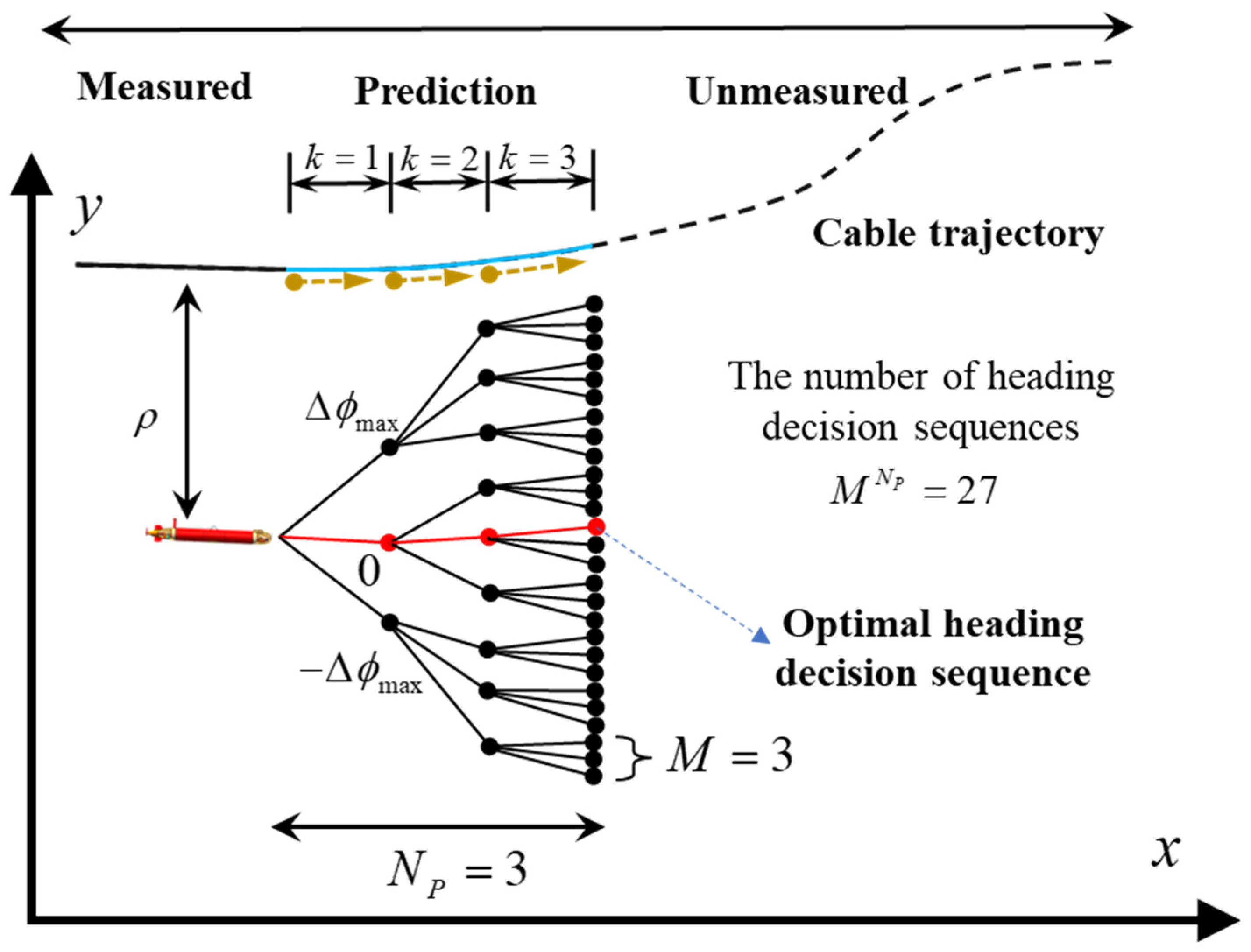
4.2.2. Non-Myopic Optimization Algorithm

After establishing the objective function, a dynamic programming method can be employed to solve the optimization problem within a finite planning horizon. As described above, the heading is the only control variable. A decision tree is created by discretizing the possible heading changes of the AUV over future time steps, with the optimal AUV heading sequence corresponding to the branch that has the lowest cost.

To avoid drastic changes, the heading changes of the AUV at each future step can be constrained within the $\left[-\mathsf{\Delta }{\varphi }_{max},\mathsf{\Delta }{\varphi }_{max}\right]$ limits. The discretized heading-search space ($\xi$) for each step can be expressed as follows:

$$\xi =\left[-\mathsf{\Delta }{\varphi }_{max},-\mathsf{\Delta }{\varphi }_{max}+{\varphi }_{res},\dots ,{-\varphi }_{res},0,{\varphi }_{res},\dots ,\mathsf{\Delta }{\varphi }_{max}-{\varphi }_{res},\mathsf{\Delta }{\varphi }_{max}\right]$$

(13)

where ${\varphi }_{res}$ denotes the resolution of the heading change and M denotes the size of $\xi$, expressed as follows:

$$M=⌊2\mathsf{\Delta }{\varphi }_{max}/{\varphi }_{res}⌋+1$$

(14)

where $⌊·⌋$ is rounded up. A smaller ${\varphi }_{res}$ indicates a finer AUV heading control and a larger M.

As shown in Figure 9, each node in the decision tree can generate M child nodes, with the state of each child node corresponding to a possible heading decision $\mathsf{\Delta }{\psi }_i$, $\mathsf{\Delta }{\psi }_i\in \xi$. For the decision tree with N_p prediction steps, a decision domain ($\gamma$) with $M^{N_P}$ possible heading decision sequences can be generated. Figure 9 shows a decision tree with N_p = 3 and M = 3.

Here, we seek a sequence of decisions ${\psi }_{opt}=[\mathsf{\Delta }{\psi }_1,\mathsf{\Delta }{\psi }_2,\cdots ,\mathsf{\Delta }{\psi }_{N_P}]$ that minimizes the cumulative cost $J\left(\psi \right)$, as defined in Equation (15). This sequence corresponds to the lowest-cost branch of the tree. Thus, the optimization problem can be transformed into finding the sequence of heading decisions that minimizes the $J\left(\psi \right)$.

$${\psi }_{opt}=\underset{\psi \in \gamma }{argmin}J(\psi ).$$

(15)

This is a discrete optimization problem for selecting the least costly sequence of AUV headings over the set of possible sequences for AUV heading decisions. When the optimal sequence is determined, the first heading in the sequence is used to control the AUV. This optimization search process is repeated when the AUV detects a new cable state, the process of which is presented in Algorithm 1.

Algorithm 1: Non-myopic cable-tracking algorithm

Input: $$\begin{gathered} \mathrm{The}\mathrm{predicted}\mathrm{cable}\mathrm{state}[s_1,s_1,\cdots ,s_{N_p}],\mathrm{AUV}\mathrm{current}\mathrm{state}\left[x,y,{\psi }_0\right],\mathrm{the}\mathrm{heading}\text{-}\mathrm{change}\mathrm{resolution}{\varphi }_{res},\mathrm{and}\mathrm{the}\mathrm{space}\mathrm{of}\mathrm{heading}\mathrm{constraints}\left[-\mathsf{\Delta }{\varphi }_{max},\mathsf{\Delta }{\varphi }_{max}\right]; \\ \mathbf{Output}\mathbf{:} \\ \mathrm{AUV}\mathrm{optimal}\mathrm{heading}\text{-}\mathrm{decision}\mathrm{sequence}{\psi }_{opt}=[\mathsf{\Delta }{\psi }_1,\mathsf{\Delta }{\psi }_2,\cdots ,\mathsf{\Delta }{\psi }_{N_P}]; \end{gathered}$$ (1) $\mathrm{Discretize}\mathrm{the}\mathrm{AUV}\mathrm{heading}\text{-}\mathrm{decision}\mathrm{space}\mathrm{and}\mathrm{compute}\xi$; (2) $\mathrm{Predict}\mathrm{the}\mathrm{state}\mathrm{of}\mathrm{the}\mathrm{AUV}\mathrm{for}\mathrm{the}\mathrm{next}{N}_P$ steps based on the given sequence of heading decisions:       (1) $\mathrm{Calculate}\mathrm{the}\mathrm{heading}\mathrm{for}\mathrm{the}\mathrm{next}{N}_P\mathrm{steps}\mathrm{of}\mathrm{the}\mathrm{AUV}:{\psi }_{k+1}={\psi }_k+\mathsf{\Delta }{\psi }_i$, $i\le N_P$;       (2) Predict the AUV position by combining the kinematic model (Equation (1)): $\left[\begin{array}{c}{x}_{k+1}\\ y_{k+1}\end{array}\right]=\left[\begin{array}{c}{x}_k\\ y_k\end{array}\right]+\left[\begin{array}{c}\mathit{sin}({\psi }_k)u\\ \mathit{cos}({\psi }_k)u\end{array}\right]T+\left[\begin{array}{c}{w}_x\\ w_y\end{array}\right]$, where u denotes the axial velocity of the AUV; (3) $\mathrm{Calculate}\mathrm{the}\cos \mathrm{t}\mathrm{of}\mathrm{each}\mathrm{heading}\text{-}\mathrm{decision}\mathrm{sequence}:J\left(\psi \right)={\omega }_1{f}_1\left(\psi \right)+{\omega }_2{f}_2\left(\psi \right)+{\omega }_3{f}_3\left(\psi \right)$; (4) $$\begin{gathered} \mathrm{Find}\mathrm{the}\mathrm{least}\cos \mathrm{tly}\mathrm{sequence}\mathrm{of}\mathrm{heading}\mathrm{decisions}:{\psi }_{opt}=\underset{\psi \in \gamma }{argmin}J(\psi ); \\ \mathbf{Return}{\psi }_{opt}; \end{gathered}$$

4.3. Strategies for Solving Non-Myopic Optimization Problems

While the non-myopic RHO strategy enhances tracking performance, an exhaustive search becomes computationally expensive and time-consuming as the number of prediction steps increases, making it impractical for real-time operation on unmanned platforms. This section exploits the specificity of SSS cable tracking to improve search efficiency by dynamically adjusting the heading-search space and pruning the decision tree.

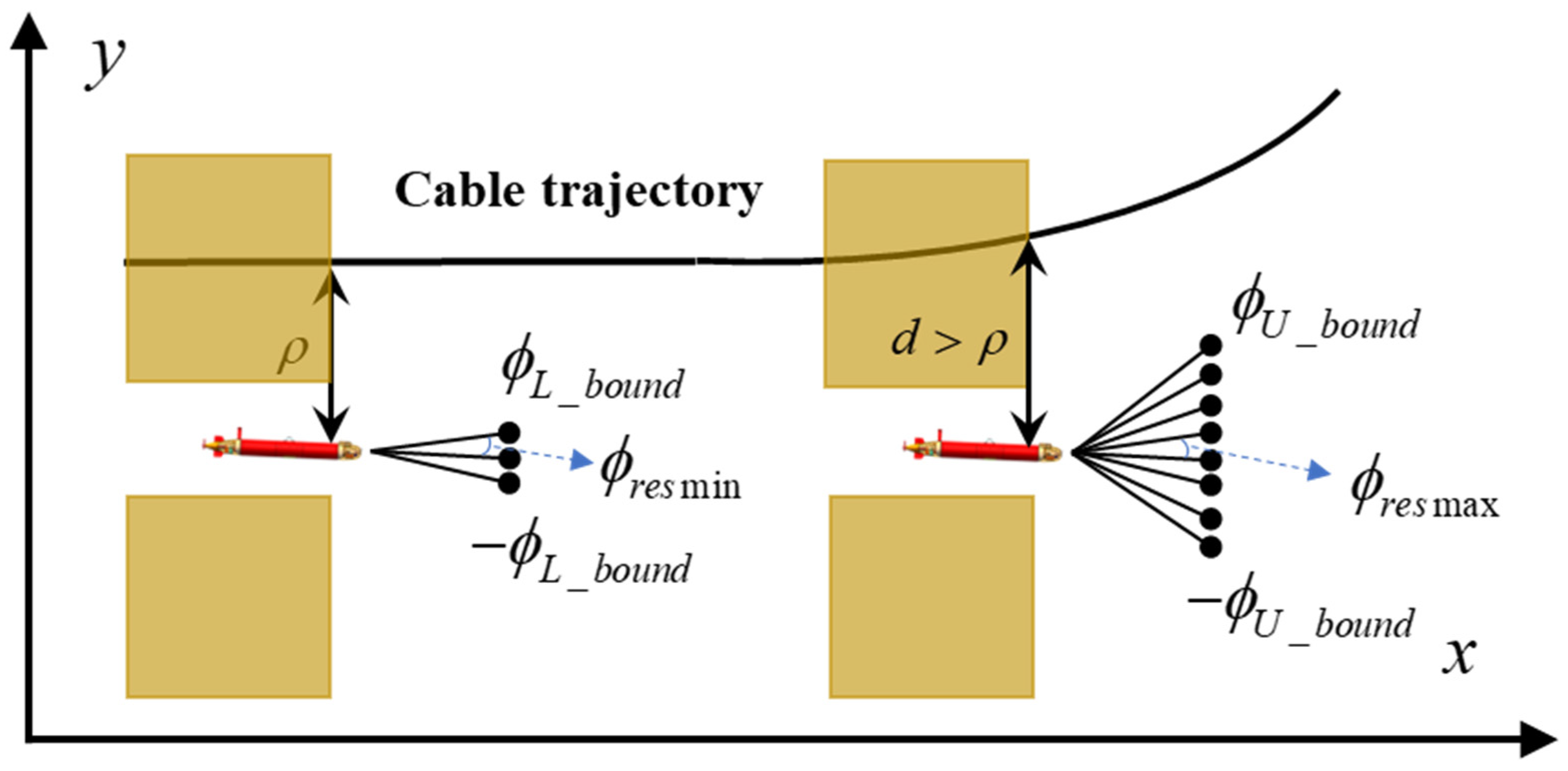
4.3.1. Adaptive Heading-Search Space Method

Considering that AUVs may encounter different scenarios during cable tracking, a fixed $\mathsf{\Delta }{\varphi }_{max}$ throughout the entire task may not optimize the algorithmic performance. Consequently, the search speed can be improved by dynamically adjusting the size and resolution of the heading-decision space. $\mathsf{\Delta }{\varphi }_{max}$ and ${\varphi }_{res}$ are two key parameters that determine the size of the search space (M). Their selection directly affects the computational complexity and precision of path planning. A reduction in the number of heading-decision sequences $M^{N_P}$ means an increase in speed, and a smaller ${\varphi }_{res}$ ensures more accurate AUV cable tracking.

As shown in Figure 10, when the relative position between the AUV and the cable approaches its optimal position, the AUV need only search the heading within a smaller range to meet the tracking requirements. Defining $\mathsf{\Delta }{\varphi }_{max}$ as expressed in Equation (16) ensures not only meeting the turning requirements but also preventing significant distortion of the sonar image. Moreover, a smaller resolution ${\varphi }_{res}$ is required to facilitate fine control. When the state between the AUV and the cable significantly deviates from the optimal imaging condition and the cable is about to exit the SSS’s field of view, the AUV may require a larger turning angle to bring the cable back into the optimal observation region. Consequently, to avoid increasing the number of searches, a larger ${\varphi }_{res}$ can be selected.

Before each heading optimization, it is necessary to analyze the current relative states between the AUV and cable, including the relative distance (d) and relative angle (φ). The specific rules can be expressed as follows:

$$\left\{\begin{array}{c}\mathsf{\Delta }{\varphi }_{max}={\varphi }_{L\_bound}and{\varphi }_{res}={\varphi }_{resmin},ifd\le di{s}_{thres}and\phi \le {\psi }_{thres}\\ \mathsf{\Delta }{\varphi }_{max}={\varphi }_{U\_bound}and{\varphi }_{res}={\varphi }_{resmax},ifd>di{s}_{thres}and\phi >{\psi }_{thres}\end{array}\right.,$$

(16)

where ${\varphi }_{L\_bound}$ and ${\varphi }_{U\_bound}$ denote the boundaries of $\mathsf{\Delta }{\varphi }_{max}$; ${\varphi }_{resmin}$ and ${\varphi }_{resmax}$ denote the maximum and minimum resolutions, respectively; $di{s}_{thres}$ and ${\psi }_{thres}$ denote the thresholds corresponding to the distance and angle, respectively.

4.3.2. Tree Search and Pruning Algorithms

The pruning algorithm is one of the more important tools for reducing the computational burden of the optimization search process. To minimize the unnecessary back-and-forth movements of the AUV, it is necessary to consider the heading changes between adjacent steps. Specifically, if the heading change selected in the ith step exceeds $\mathsf{\Delta }{\psi }_{thres}$, a larger heading change in the opposite direction in the (i + 1)th step is not allowed. In other words, decision nodes with an angular decrease greater than $-2\mathsf{\Delta }{\psi }_{thres}$ in the (i + 1)th step are pruned. This approach functions similarly to Equation (9), where f₁ is used to reduce the number of decision sequences by pruning unnecessary branches. It should be noted that the closer $\mathsf{\Delta }{\psi }_{thres}$ is to $\mathsf{\Delta }{\psi }_{max}$, the less obvious the trimming effect, and vice versa, resulting in an inadequate search process.

The branch-and-bound method is another pruning technique [39]. Several concepts used by this algorithm must be clarified. The nodes for which the cost has already been computed are referred to as open nodes. If all child nodes of such a node are in the “open” state, then the status of this node is considered to be expanded. The search process of a decision tree is essentially a sequence of node expansions. This method leverages the tree structure and additivity of sequence costs to set lower bounds for the costs of all nodes in the tree. The lower bound of a node can be defined as the cost of the nearest ancestral node. During the node-expansion process, any node whose lower bound exceeds the cost of the current best-decision sequence is removed from the tree. Removing a node implies pruning it, meaning that neither it nor its sub-nodes will participate in the search for the optimal decision sequence [22,40].

The core idea of the branch-and-bound algorithm for searching decision trees can be summarized as follows, with the pseudocode presented in Algorithm 2.

(1)

Initialize the minimum cost $J_{min}$, perform a uniform cost search (UCS), and expand the nodes until reaching the end node of the tree (at a depth of $N_P$). Set the decision sequence with the lowest cost as the initial optimal solution and set $J_{min}$ to the cost of that decision sequence. Repeat until all nodes in the tree are opened.

(2)

During node expansion, the lower bound is compared with $J_{min}$, and nodes with lower bounds greater than or equal to $J_{min}$ are pruned. If the search for nodes is completed (end nodes are opened) and the corresponding decision sequence cost is lower than $J_{min}$, the decision sequence is considered the new best-decision sequence and $J_{min}$ is set as the cost of the sequence.

Algorithm 2: Branch-and-bound algorithm

(1) $\mathrm{Initialize}:J_{min}=\infty$; (2) $\mathrm{Execute}\mathrm{the}\mathrm{UCS}\mathrm{and}\mathrm{expand}\mathrm{the}\mathrm{node}\mathrm{until}\mathrm{it}\mathrm{reaches}\mathrm{the}\mathrm{depth}{N}_P$; (3) $\mathrm{Set}\mathrm{the}\mathrm{least}\cos \mathrm{tly}\mathrm{decision}\mathrm{sequence}{\psi }_{local\_opt}$$\mathrm{as}\mathrm{the}\mathrm{initial}\mathrm{optimal}\mathrm{solution}\mathrm{and}\mathrm{update}{J}_{min}$ to $J\left({\psi }_{local\_opt}\right)$; (4) $\mathrm{Opened}\mathrm{but}\mathrm{unexpanded}\mathrm{nodes}\mathrm{with}\mathrm{a}\mathrm{depth}\mathrm{less}\mathrm{than}{N}_P$$\mathrm{are}\mathrm{listed}\mathrm{in}\mathrm{the}\mathrm{list}R$ in ascending order of cost; (5) While there is a node in the list Do     Expands the first node in the list R;     If the sequence corresponding to a node has a cost >Jmin         Stop the expansion of the node;         Remove it from R;     End     If the depth of the children of this node == NP         If decision sequence costs with minimum costs $$\begin{gathered} J_{min}=J\left({\psi }_{local\_opt}\right) \\ \mathrm{Consider}{\psi }_{local\_opt}\mathrm{as}\mathrm{the}\mathrm{optimal}\mathrm{decision}\mathrm{sequence}; \\ \mathbf{End} \\ \mathbf{Else} \\ \mathrm{Sort}\mathrm{the}\mathrm{children}\mathrm{of}\mathrm{this}\mathrm{node}\mathrm{in}\mathrm{ascending}\mathrm{order}\mathrm{in}\mathrm{the}\mathrm{list}R; \\ \mathbf{End} \\ (6)\mathbf{Return}\mathrm{Optimal}\mathrm{Decision}\mathrm{Sequence}{\psi }_{opt}={\psi }_{local\_opt}; \end{gathered}$$

5. Simulation and Discussion

To validate the effectiveness of the proposed method, we used MATLAB 2019a to establish a complex cable model based on potential trajectories during actual laying, focusing on analyzing the tracking capability of the method. A cable detection method based on sonar images is beyond the scope of this study. Here, we simplify the SSS measurement model of SSS using circular regions.

5.1. Simulation Setup and Environment

Submarine cables are generally placed along straight trajectories. However, under special circumstances—such as when avoiding complex terrain and obstacles, protecting underwater ecological resources, preventing geological subsidence, or reducing cable tension—engineers can develop appropriate laying plans based on the specific environmental conditions and technical specifications of the cable, to ensure its stability and reliability. For example, to address the impact of geological subsidence on the normal operation of submarine pipelines, the authors of Ref. [41] laid flexible pipes with a certain curvature to enhance their adaptability to the environment. To ensure that our cable prediction and tracking experiments were more credible, we constructed a complex submarine cable model containing both straight and curved segments. The cable’s state sequence consisted of 7820 entries, with states represented by depth, longitude, latitude, and heading angle, as detailed in

Table 1. Cable status data format.

Samples	Depth	Longitude	Latitude	Angle
7820	20 m	123.65821E	41.93709N	74°

. In this study, we assumed the cable was laid flat on the seabed without burial or suspension and that the seabed substrate type was homogeneous.

Figure 11 illustrates a two-dimensional representation of the cable model on the seabed, featuring a rectangular search area (SABCD) measuring 800 × 250 m, as indicated by the gray area in the figure. The northeast coordinate system XOY was established with point A as the origin, which was used to characterize the relative positions of the points within the region. The World Geodetic System (WGS-84) was used to convert the latitude and longitude of the points in the region [42]. The length and curvature radius of each segment of the cable are listed in

Table 2. Cable length and curvature radius of each cable segment.

Label	${\mathit{L}}_1$	${\mathit{R}}_1$	${\mathit{L}}_2$	${\mathit{R}}_2$	${\mathit{L}}_3$	${\mathit{R}}_3$	${\mathit{L}}_4$	${\mathit{R}}_4$	${\mathit{L}}_5$	${\mathit{R}}_5$	${\mathit{L}}_6$
Radius of curvature/Length (m)	50	35	75	45	125	70	71	59	166	82	135

.

The AUV motion—treated as a mass point—is guided by the “Sea Whale” AUV’s dynamic model and parameters [43], as indicated by the red dot in the figure. The simplified SSS measurement model is represented by the red dashed circular region (radius of 30 m) in the figure. The red highlighted area in the figure represents the imaging of the cable in the sonar image, with its state determined by detecting the overlap between the circular area and the cable in real time. For clarity, the yellow regions (30 m wide) on both sides are defined as the effective AUV measurement area, where the cable remains within the SSS field of view when the AUV is in this region. The purple regions (3 m wide) on both sides are measurement blind zones, where the cable is in the SSS blind spot when the AUV operates in this area. The magenta dotted line, located 15 m from the cable, is defined as the best tracking line, ensuring that the cable stays within the SSS optimal observation area during movement along this line.

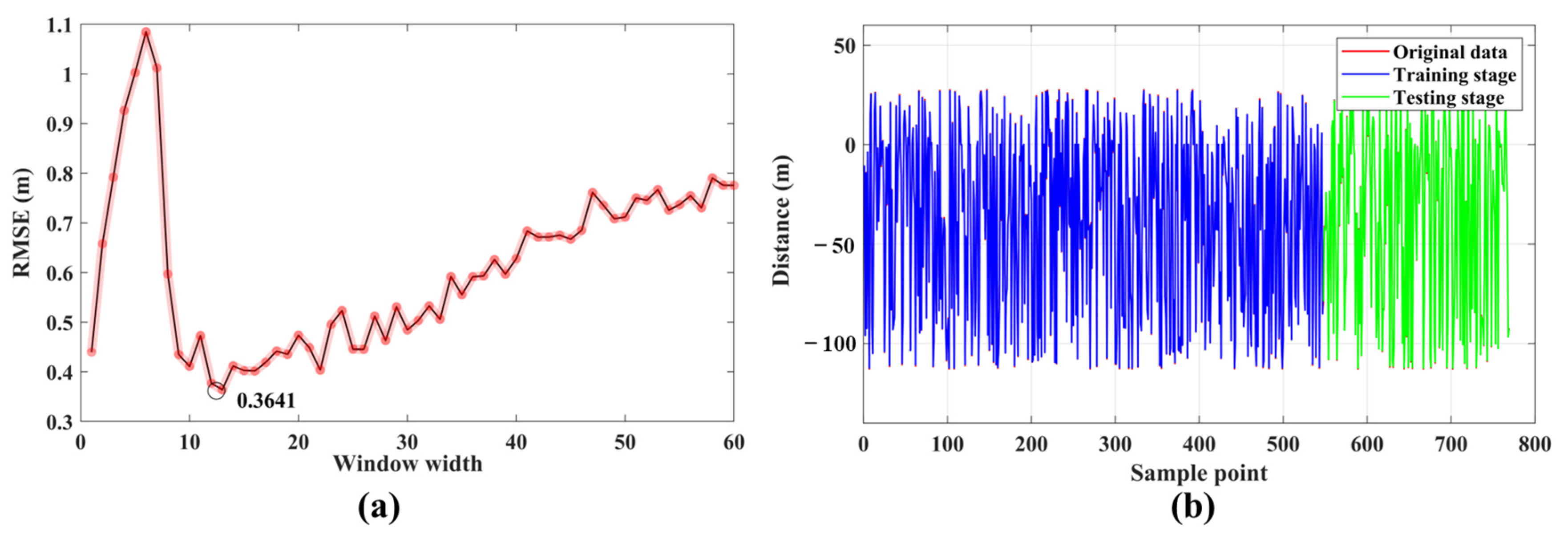
5.2. The Results of Cable State Prediction

The cable state prediction model was trained using the obtained dataset. The root mean square error (RMSE) was used as a performance metric to indicate the prediction accuracy. Specifically, 70% of the total sample size was allocated for training, while 30% was set aside for testing. The optimization function used the Adaptive Moment Estimation method (Adam), which iteratively minimized the loss function.

Table 3. LSTM network parameters.

Hyperparameters	Description	Value
numHiddenUnits	Number of hidden units	40
MaxEpochs	Number of training rounds	400
MiniBatchsize	Minimum batch number of samples	26
InitialLearnRate	Initial learning rate	0.005
LearnRateDropPeriod	Learn rate drop period	200
LearnRateDropFactor	Learn rate drop factor	0.1

lists the LSTM network parameters.

To achieve a better prediction performance, various sliding window sizes were selected for comparative experiments, with the window size t set from 1 to 60, using a sliding step of 1. The test results are shown in Figure 12a, which illustrates the distribution of the RMSE under different sliding window sizes. The RMSE curve indicates that the size of the sliding window significantly impacts the predictive performance of the model. A smaller window fails to capture sufficient historical information, while an excessively large window introduces noise, reducing the prediction accuracy. Experimental results demonstrate that a window size of t = 13 strikes the optimal balance between utilizing historical data and minimizing noise, achieving the best predictive performance with a minimum RMSE of 0.3641 m.

For a sample size of 7820, setting the window size to 13 and the step size to 1 resulted in 7808 new samples. Figure 12b shows the prediction performance of the LSTM network for the cable states for t = 13. The red, blue, and green lines represent the original data, the prediction results of the training dataset, and the prediction results of the testing dataset, respectively. The prediction results align well with the actual data, especially in the testing phase, where the model showed strong predictive performance. This suggests that the model has good generalization ability, making it effective for cable state prediction tasks.

5.3. Tracking Performance and Method Comparison

The initial state of the AUV is $\left[x\right(0),y(0),u(0),v(0\left)\right]=[\mathrm{123.649042,41.936137,0}\mathrm{m}/\mathrm{s},0\mathrm{m}/\mathrm{s}]$, which is shown as a hollow red dot in Figure 13.

The thruster rotational speed was 120 rpm, which ensured that the axial speed of the AUV reached 1 m/s. The SSS measurement range was 30 m, with a sampling period of T = 2 s. The experiment adopted the automatic cable-tracking method framework described in a previous study [13] to autonomously search and track the cable. The search mode adopted a lawnmower pattern with a spacing of w = 40 m, and, once a cable was detected, the AUV switched to tracking mode. Furthermore, it is important to note that the simulation assumes a uniform seabed environment without complex obstacles or varying water flow, enabling the AUV to respond immediately to cable signals upon detection. In actual operations, the environment can be much more complex, which is a significant difference from the simulation. To verify the effectiveness of the proposed method, we compared it with a line-of-sight (LOS)-based guidance method and analyzed the impact of the proposed method on tracking performance under different $\mathsf{\Delta }{\varphi }_{max}$ constraints. Finally, five metrics were used to evaluate the performance—that is, the mean distance (MD), distance standard deviation (SD), mean angle (MA), the angle’s standard deviation (SA), and standard deviation of the AUV heading-angle change (SH), where MD and SD are the embodiment of the distance between the AUV and the cable, MA and SA are used to measure the degree of parallelism between the AUV and the cable, and SH characterizes the smoothness of the AUV motion.

5.3.1. Tracking Performance Analysis

Figure 13 shows the AUV cable-tracking trajectory when guided by different methods. The AUV starts from the deployment point, chooses point A as a nearby starting point, and performs the cable-searching task. The tracking behavior is triggered when the AUV detects the cable, and the goal distance between the cable and the AUV is set to ρ = 15 m. As shown in Figure 13, the LOS-based method converges more quickly to the cable trajectory initially (e.g., at P1), but its “short-sighted” nature leads to significant oscillations during tracking, particularly at P2 and P3. These oscillations create instability in the AUV’s motion, potentially affecting cable tracking and SSS imaging quality. In contrast, the proposed method generates a smoother trajectory by predicting and adjusting the AUV’s future heading. At P2 and P3, the AUV aligns better with the cable, reducing oscillations and enhancing tracking stability and smoothness.

Figure 14 shows the results of the different methods during the tracking phase. Figure 14a shows the AUV heading-angle curve, Figure 14b shows the distance between the AUV and cable, Figure 14c shows the difference between the AUV heading angle and the cable direction angle, and Figure 14d shows the AUV heading variation.

Table 4. Performance comparison of the three methods.

Method	MD (m)	SD (m)	MA (°)	SA (°)	SH (°)
$\mathrm{New}\mathrm{method}\mathsf{\Delta }{\phi }_{max}=4\circ$	1.5	1.07	1.37	1.81	0.17
$\mathrm{New}\mathrm{method}\mathsf{\Delta }{\phi }_{max}=10\circ$	0.69	0.34	1.22	1.72	0.22
LOS-based method	0.89	0.65	6.93	3.92	0.62

provides a quantitative comparison of the various indicators.

A detailed analysis reveals that the proposed optimization method significantly outperforms the LOS method in terms of both tracking error and trajectory stability. Specifically, at Δφ_max = 10°, the proposed method greatly reduces the average distance between the AUV and the cable (MD = 0.69 m) and minimizes fluctuation (SD = 0.34 m), demonstrating superior tracking accuracy. In contrast, the LOS method shows higher values (MD = 0.89 m, SD = 0.65 m), indicating poorer tracking performance, especially in complex path scenarios.

In terms of trajectory stability, the proposed method reduces the deviation between the AUV’s heading and the cable direction (SA = 1.72°), while the LOS method exhibits significantly larger deviations (SA = 3.92°), leading to greater instability. Additionally, with Δφ_max = 4°, the proposed method minimizes heading-angle variations (SH = 0.17°), resulting in smoother trajectories, whereas the LOS method displays greater oscillations (SH = 0.62°).

Overall, the proposed method offers better control over tracking error and trajectory smoothness, ensuring more precise cable tracking and reducing the frequency of abrupt adjustments. These improvements enhance SSS imaging quality and reduce the likelihood of losing the cable during complex tracking tasks.

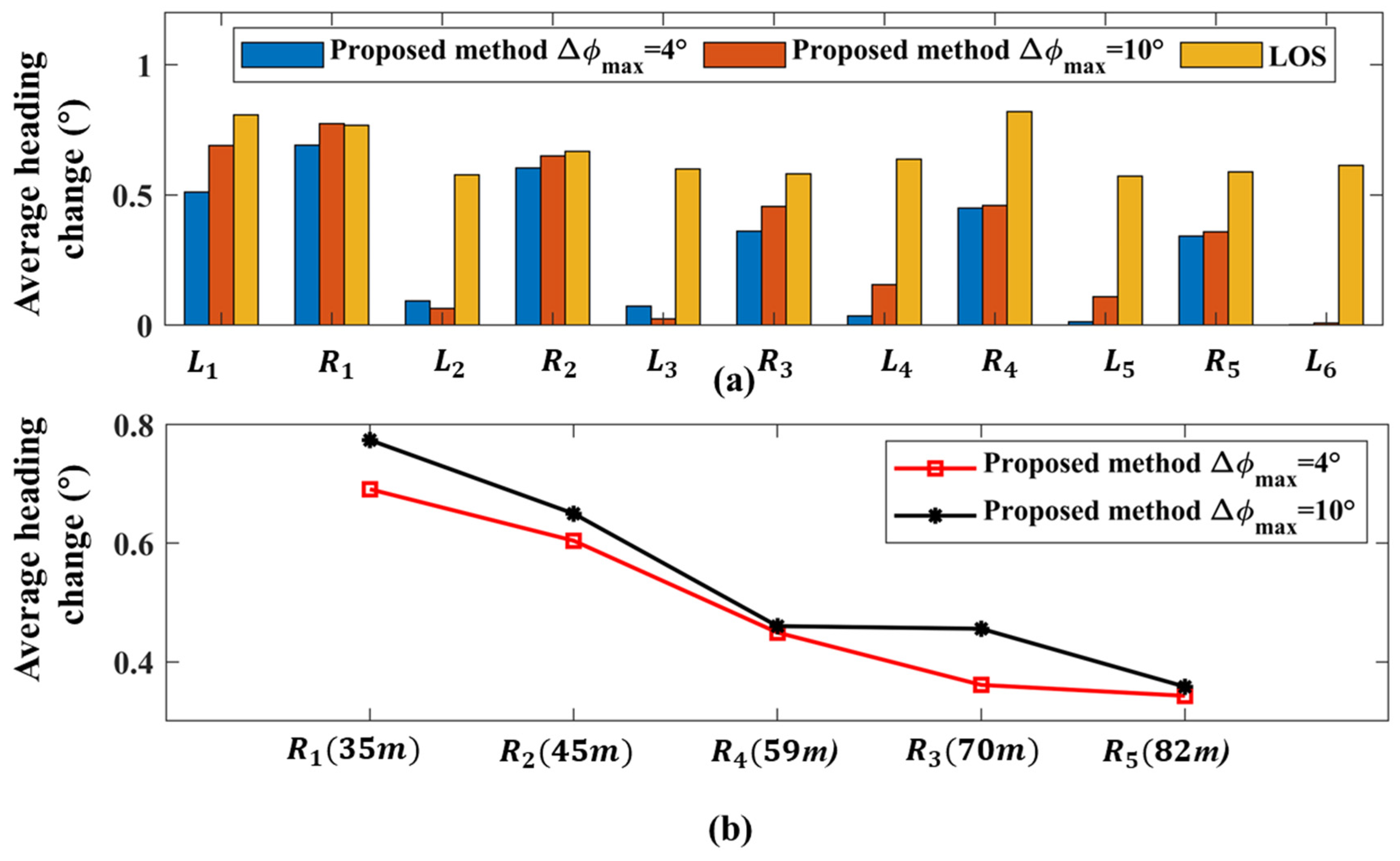
5.3.2. Impact of Cable Curvature on AUV Stability

Based on a macroscopic description of performance, Figure 15a shows a bar chart of the mean AUV heading-angle variation in the different cable segments. The proposed method exhibits superior navigation stability when tracking straight-line cables. Figure 15b shows that the stability of the AUV is inversely proportional to the curvature radius. The smaller the curvature radius, the more severe the heading oscillation of the AUV, which results in poorer SSS imaging. Moreover, lower $\mathsf{\Delta }{\varphi }_{max}$ values lead to better navigational stability under the guidance of the proposed method.

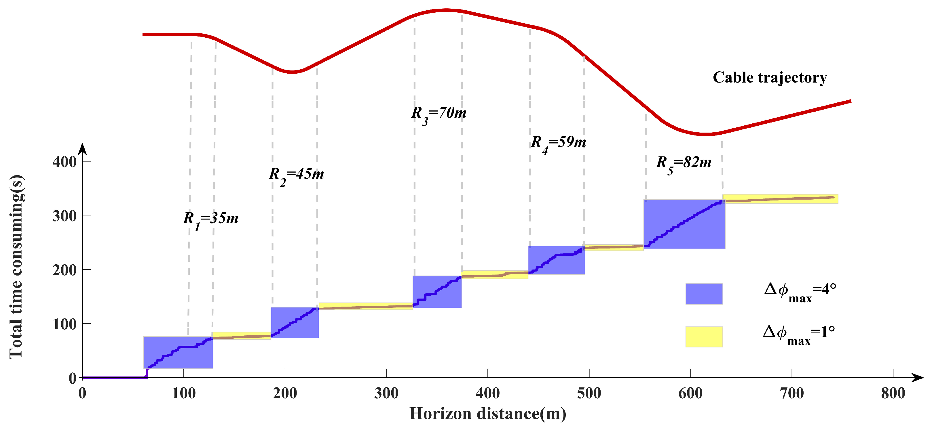
5.3.3. Time-Consumption Analysis

We used Δφ_max = 4° as an example to analyze the performance of the decision tree simplification strategy, the key parameters of which are listed in

Table 5. Decision tree optimization simplification settings.

Number	Parameters	Value	Number	Parameters	Value
1	${dis}_{thres}$	4 m	5	${\varphi }_{resmin}$	0.5°
2	${\psi }_{thres}$	4°	6	${\varphi }_{resmax}$	1°
3	${\varphi }_{L\_bound}$	1°	7	$\mathsf{\Delta }{\psi }_{thres}$	0.5*Δφmax
4	${\varphi }_{U\_bound}$	4°	8	$N_P$	5

.

Without simplification, the depth of the decision tree is $N_P=5$, with the size of the heading-search space being M = 9, and there are 59,049 decision sequences in each heading search. The total time taken to find the optimal decision sequences throughout the tracking process is as much as 2541 s. With the application of the decision tree simplification method, the total computational time for searching the optimal heading sequence is reduced to 361 s, achieving a seven-fold speedup.

Figure 16 illustrates the distribution of total optimization computation time throughout the entire process, indicating that tracking a straight-line cable requires fewer computational resources compared to a curved cable. The purple and yellow areas represent the distribution of the AUV’s operating time on straight and curved paths, respectively. This is because tracking straight cables satisfies the conditions of Equation (16) by adjusting certain parameters where $\mathsf{\Delta }{\varphi }_{max}=\mathsf{\Delta }{\varphi }_{L\_bound}$ and ${\varphi }_{res}={\varphi }_{resmin}$ (M = 5), resulting in a maximum of 3125 decision sequences in each heading search. With the same pruning strategy, reducing M can dramatically improve the search efficiency.

6. Conclusions and Future Work

Existing cable-tracking strategies have not addressed the control of AUVs to optimize the sensing capabilities of onboard sensors for better target inspection. This study examined the problem of underwater cable tracking using SSS-equipped AUVs, focusing on achieving the stable and continuous tracking of cables with complex trajectories while optimizing imaging quality. Based on the SSS imaging characteristics, this study summarized three key factors affecting the SSS image quality and proposed a non-myopic RHO model. The proposed model used LSTM networks to predict cable trends, thereby improving the subsequent tracking accuracy. To adapt the model to embedded systems, this study reduced the computational complexity by shrinking the heading-search space and pruning the decision tree. Experimental results indicated that, compared to traditional methods, the proposed non-myopic approach achieved more stable and continuous tracking of underwater cables with complex trajectories while maintaining the low algorithmic computational complexity suitable for embedded systems. Further analysis revealed that AUV motion constraints affect navigation stability; specifically, limiting the heading search space can reduce heading oscillations, albeit at the expense of distance and angle performance. Additionally, the stability of AUV cable tracking was found to be inversely proportional to the curvature radius, with a smaller curvature radius leading to more pronounced heading oscillations. This study evaluated the imaging quality of cables in SSS at the theoretical level by quantifying AUV motion performance indicators. However, it overlooked the impact of target characteristics, the underwater environment, and SSS parameters on cable tracking in practical applications. In addition, depth control of the AUV in the vertical plane is currently neglected in favor of horizontal motion. In the future, we aim to apply the model to real-world cable inspection tasks, analyze the technical details further, and gradually optimize the model to enable the efficient autonomous inspection of submarine cables.

References

1. Bueger, C.; Liebetrau, T.; Franken, J. In-Depth Analysis Requested by the SEDE Sub-Committee Security Threats to Undersea Communications Cables and Infrastructure—Consequences for the EU; European Parliament: Strasbourg, France, 2022. [Google Scholar] [CrossRef]
2. Gheorghe, A.V.; Vamanu, D.V.; Katina, P.F. Critical Infrastructures, Key Resources, Key Assets; Springer: Cham, Switzerland, 2018; ISBN 9783319692234. [Google Scholar]
3. Adegboye, M.A.; Fung, W.; Karnik, A. Recent Advances in Pipeline Monitoring and Oil Leakage Detection Technologies: Principles and Approaches. Sensors 2019, 19, 2548. [Google Scholar] [CrossRef] [PubMed]
4. Gritzalis, D.A. Cyber-Attacks on the Oil & Gas Sector: A Survey on Incident Assessment and Attack Patterns. IEEE Access 2020, 8, 1–37. [Google Scholar] [CrossRef]
5. Shama, A.M.; El-Rashid, A.; El-Shaib, M.; Kotb, D.M. Review of Leakage Detection Methods for Subsea Pipeline. Marit. Transp. Harvest. Sea Resour. 2018, 2, 1141–1149. [Google Scholar]
6. Jacobi, M.; Karimanzira, D. Multi Sensor Underwater Pipeline Tracking with AUVs. In Proceedings of the Oceans 2014 MTS/IEEE, St. John’s, NL, Canada, 14–19 September 2014; pp. 2–7. [Google Scholar] [CrossRef]
7. Littlefield, R.H.; Soenen, K.; Packard, G.; Kaeli, J. Seafloor Cable Based Navigation and Monitoring with Autonomous Underwater Vehicles. In Proceedings of the Oceans 2019 MTS/IEEE, Seattle, WA, USA, 27–31 October 2019. [Google Scholar] [CrossRef]
8. Bobkov, V.; Shupikova, A.; Inzartsev, A. Recognition and Tracking of an Underwater Pipeline from Stereo Images during AUV-Based Inspection. J. Mar. Sci. Eng. 2023, 11, 2002. [Google Scholar] [CrossRef]
9. Zhang, J.; Xiang, X.; Li, W. Adaptive Neural Control of Flight-Style AUV for Subsea Cable Tracking Under Electromagnetic Localization Guidance. IEEE/ASME Trans. Mechatron. 2023, 28, 2976–2987. [Google Scholar] [CrossRef]
10. Szyrowski, T.; Sharma, S.K.; Sutton, R.; Kennedy, G.A. Developments in Subsea Power and Telecommunication Cables Detection: Part 1–Visual and Hydroacoustic Tracking. Underw. Technol. 2013, 31, 123–132. [Google Scholar] [CrossRef]
11. Evans, J.; Patron, P.; Privat, B.; Johnson, N.; Capus, C. AUTOTRACKER: Autonomous Inspection–Capabilities and Lessons Learned in Offshore Operations. In Proceedings of the Oceans ’09 MTS/IEEE Biloxi–Marine Technology for Our Future: Global and Local Challenges, Biloxi, MI, USA, 26–29 October 2009. [Google Scholar] [CrossRef]
12. Xiang, X.; Yu, C.; Niu, Z.; Zhang, Q. Subsea Cable Tracking by Autonomous Underwater Vehicle with Magnetic Sensing Guidance. Sensors 2016, 16, 1335. [Google Scholar] [CrossRef]
13. Feng, H.; Yu, J.; Huang, Y.; Cui, J.; Qiao, J. Automatic Tracking Method for Submarine Cables and Pipelines of AUV Based on Side Scan Sonar. Ocean Eng. 2023, 280, 114689. [Google Scholar] [CrossRef]
14. El-Fakdi, A.; Carreras, M. Policy Gradient Based Reinforcement Learning for Real Autonomous Underwater Cable Tracking. In Proceedings of the 2008 IEEE/RSJ International Conference on Intelligent Robots and Systems IROS, Nice, France, 22–26 September 2008; pp. 3635–3640. [Google Scholar] [CrossRef]
15. Zhang, Y.; Zhang, H.; Liu, J.; Zhang, S.; Liu, Z.; Lyu, E.; Chen, W. Submarine Pipeline Tracking Technology Based on AUVs with Forward Looking Sonar. Appl. Ocean Res. 2022, 122, 103128. [Google Scholar] [CrossRef]
16. Bagnitsky, A.; Inzartsev, A.; Pavin, A.; Melman, S.; Morozov, M. Side Scan Sonar Using for Underwater Cables & Pipelines Tracking by Means of AUV. In Proceedings of the 2011 IEEE Symposium on Underwater Technology, UT’11 and Workshop on Scientific Use of Submarine Cables and Related Technologies, SSC’11, Tokyo, Japan, 5–8 April 2011. [Google Scholar] [CrossRef]
17. Antich, J.; Ortiz, A. Development of the Control Architecture of an Underwater Cable Tracker. Int. J. Intell. Syst. 2005, 20, 477–498. [Google Scholar] [CrossRef]
18. Naeem, W.; And, R.S.; Ahmad, S.M. Pure Pursuit Guidance and Model Predictive Control of an Autonomous Underwater Vehicle for Cable/Pipeline Tracking. Proc. Inst. Mar. Eng. Sci. Technol. Part C J. Mar. Sci. Environ. 2004, 279–283. [Google Scholar]
19. Cai, M.; Member, S.; Wang, Y.; Wang, S.; Wang, R.; Cheng, L.; Member, S.; Tan, M. Prediction-Based Seabed Terrain Following Control for an Underwater Vehicle-Manipulator System. IEEE Trans. Syst. Man, Cybern. Syst. 2021, 51, 4751–4760. [Google Scholar] [CrossRef]
20. Shen, C.; Shi, Y.; Buckham, B. Integrated Path Planning and Tracking Control of an AUV: A Unified Receding Horizon Optimization Approach. IEEE/ASME Trans. Mechatron. 2017, 22, 1163–1173. [Google Scholar] [CrossRef]
21. Cao, X.; Ren, L.; Sun, C. Dynamic Target Tracking Control of Autonomous Underwater Vehicle Based on Trajectory Prediction. IEEE Trans. Cybern. 2023, 53, 1968–1981. [Google Scholar] [CrossRef]
22. Ferri, G.; Munafo, A.; Lepage, K.D. An Autonomous Underwater Vehicle Data-Driven Control Strategy for Target Tracking. IEEE J. Ocean. Eng. 2018, 43, 323–343. [Google Scholar] [CrossRef]
23. Paull, L.; Saeedi, S.; Seto, M.; Li, H. Sensor-Driven Online Coverage Planning for Autonomous Underwater Vehicles. IEEE/ASME Trans. Mechatron. 2013, 18, 1827–1838. [Google Scholar] [CrossRef]
24. Williams, D.P. AUV-Enabled Adaptive Underwater Surveying for Optimal Data Collection. Intell. Serv. Robot. 2012, 5, 33–54. [Google Scholar] [CrossRef]
25. Cai, C.; Chen, J.; Yan, Q.; Liu, F.; Zhou, R. A Prior Information-based Coverage Path Planner for Underwater Search and Rescue Using Autonomous Underwater Vehicle (AUV) with Side-scan Sonar. IET Radar Sonar Navig. 2022, 16, 1225–1239. [Google Scholar] [CrossRef]
26. Lee, E.M. Geomorphological Mapping. Geol. Soc. Lond. Eng. Geol. Spec. Publ. 2001, 18, 53–56. [Google Scholar] [CrossRef]
27. Dondurur, D. Acquisition and Processing of Marine Seismic Data; Elsevier: Amsterdam, The Netherlands, 2018; ISBN 0128114916. [Google Scholar]
28. Paull, L.; Saeedi, S.; Li, H.; Myers, V. An Information Gain Based Adaptive Path Planning Method for an Autonomous Underwater Vehicle Using Sidescan Sonar. In Proceedings of the 2010 IEEE International Conference on Automation Science and Engineering, Toronto, ON, USA, 21–24 August 2010; pp. 835–840. [Google Scholar] [CrossRef]
29. Midtgaard, Ø.; Krogstad, T.R.; Hagen, P.E. Sonar Detection and Tracking of Seafloor Pipelines. In Proceedings of the UAM Conference, Kos, Greece, 20–24 June 2011. [Google Scholar]
30. Yordanova, V.; Gips, B. Coverage Path Planning with Track Spacing Adaptation for Autonomous Underwater Vehicles. IEEE Robot. Autom. Lett. 2020, 5, 4774–4780. [Google Scholar] [CrossRef]
31. Williams, D.P. On Optimal AUV Track-Spacing for Underwater Mine Detection. In Proceedings of the 2010 IEEE International Conference on Robotics and Automation, Anchorage, Alaska, 3–8 May 2010; pp. 4755–4762. [Google Scholar]
32. Feng, H.; Yu, J.; Huang, Y.; Qiao, J.; Wang, Z.; Xie, Z.; Liu, K. Adaptive Coverage Sampling of Thermocline with an Autonomous Underwater Vehicle. Ocean Eng. 2021, 233, 109151. [Google Scholar] [CrossRef]
33. Nie, Y.; Yang, H.; Song, D.; Huang, Y.; Liu, X.; Hui, X. A New Cross-Platform Instrument for Microstructure Turbulence Measurements. J. Mar. Sci. Eng. 2021, 9, 1051. [Google Scholar] [CrossRef]
34. Qiu, C.; Liang, H.; Huang, Y.; Mao, H.; Yu, J.; Wang, D.; Su, D. Development of Double Cyclonic Mesoscale Eddies at around Xisha Islands Observed by a ‘Sea-Whale 2000’ Autonomous Underwater Vehicle. Appl. Ocean Res. 2020, 101, 102270. [Google Scholar] [CrossRef]
35. Hu, F.; Huang, Y.; Xie, Z.; Yu, J.; Wang, Z.; Qiao, J. Conceptual Design of a Long-Range Autonomous Underwater Vehicle Based on Multidisciplinary Optimization Framework. Ocean Eng. 2022, 248, 110684. [Google Scholar] [CrossRef]
36. Qiao, J.; Yu, J.; Huang, Y.; Cui, J.; Wang, B.; Wang, Z. Sea-Whale Series AUV-Extending the Range to 4000 Kilometers. In Proceedings of the OCEANS 2022 Hampton Roads, Virtual, 17–20 October 2022. [Google Scholar] [CrossRef]
37. Hochreiter, S. Long Short-Term Memory. Neural Comput. 1997, 9, 1735–1780. [Google Scholar] [CrossRef]
38. Lei, L.; Tang, T.; Gang, Y.; Jing, G. Hierarchical Neural Network-Based Hydrological Perception Model for Underwater Glider. Ocean Eng. 2022, 260, 112101. [Google Scholar] [CrossRef]
39. Clausen, J. Branch and Bound Algorithms—Principles and Examples; University of Copenhagen: København, Demark, 1999; pp. 1–30. [Google Scholar]
40. Chhetri, A.S.; Morrell, D.; Papandreou-Suppappola, A. Nonmyopic Sensor Scheduling and Its Efficient Implementation for Target Tracking Applications. EURASIP J. Adv. Signal Process. 2006, 2006, 031520. [Google Scholar] [CrossRef]
41. Yu, Y.; Liu, F.; Jiang, J.; Liu, P.; Cui, Z. Continuous Arc-Shaped Laying Technique for Large Diameter Flexible Pipeline in Complicated Sea Conditions. Pet. Eng. Constr. 2018, 44, 36–40. [Google Scholar] [CrossRef]
42. Guowei, C.; Chen, B.M.; Lee, T.H. Unmanned Rotorcraft Systems; Springer Science & Business Media: Berlin/Heidelberg, Germany, 2011; ISBN 1852338288. [Google Scholar]
43. Huang, Y. Research on Key Technologies and Control Problems of Lightweight Long-Range AUV; University of Chinese Academy of Sciences: Beijing, China, 2020. [Google Scholar]
Figure 1. Schematic of tracking submarine cables using an AUV equipped with SSS.
Jmse 12 01725 g001
Figure 2. Schematic of the acoustic imaging of cables based on SSS.
Jmse 12 01725 g002
Figure 3. Comparison of SSS imaging effects taken in previous field measurements of the “Sea Whale” AUV. (a) Different viewing angles; (b) different lateral distances; (c) sharp turns.
Jmse 12 01725 g003
Figure 4. “Sea Whale” AUV system components.
Jmse 12 01725 g004
Figure 5. Illustration of the AUV control problem.
Jmse 12 01725 g005
Figure 6. Cable-tracking method with the Sense → Plan → Act closed-loop structure.
Jmse 12 01725 g006
Figure 7. LSTM network structure.
Jmse 12 01725 g007
Figure 8. Demonstration of the sliding prediction of the cable state.
Jmse 12 01725 g008
Figure 9. Decision tree with Np = 3 and M = 3 for cable tracking, the red sequence being the optimal heading.
Jmse 12 01725 g009
Figure 10. Diagram of the adaptive heading-search space method.
Jmse 12 01725 g010
Figure 11. Simulation environment.
Jmse 12 01725 g011
Figure 12. Evaluation of cable prediction results. (a) RMSE of the prediction results under different sliding windows. (b) Cable prediction results at t = 13.
Jmse 12 01725 g012
Figure 13. Cable-tracking results of the three methods.
Jmse 12 01725 g013
Figure 14. Series of observations made during cable tracking.
Jmse 12 01725 g014
Figure 15. AUV heading stability analysis. (a) Histogram of the mean heading change; (b) stability of the different curvature radii.
Jmse 12 01725 g015
Figure 16. Time consumption of the decision sequence search.
Jmse 12 01725 g016