Design and Implementation of a Shipborne Echo Sounder Simulator Based on a Seabed Echo Scattering and Noise Model

Abstract

The Manila Amendment 2010 to the STCW International Convention has made clear requirements for seafarers to use the navigation simulation system for training. A shipborne echo sounder is an important navigation aid equipment necessary for a ship’s bridge. Proper use of this equipment can effectively prevent ship grounding accidents. Given the lack of research on simulating different seabed substrate echoes within echo sounder simulations, this paper proposes an algorithm for generating echoes and clutter from various seabed substrates, based on the Jackson model and noise model. Using the seabed echo generation algorithm, the bathymetric data and seabed echo under the influence of ship rolling are generated, the seabed echo simulation of the sounder under the influence of four different grazing angles and six different substrates is realized. Clutter images, including random noise, bubble interference, co-frequency interference, and fish school interference, are also simulated. A typical ship echo sounder simulator is designed and developed. The echo sounder simulator developed in this paper has high realism in seabed echoes and clutter simulation, complete functions, and friendly human–computer interaction. The system has been used by college students and crews, with satisfactory results, which can effectively meet the needs of actual training of seafarers.

1. Introduction

In 2010, the International Maritime Organization (IMO) revised the International Convention on Standards of Training, Certification, and Watchkeeping for Seafarers (STCW) to enhance the professional competence and watchkeeping behavior of seafarers, reduce the impact of human factors on maritime accidents, and effectively safeguard maritime safety and property worldwide. Mandatory standards were established in Part A of this Convention, including a requirement for proficiency in the use of echo sounders, which emphasizes the need for the “Ability to operate the equipment and apply the information correctly” [1,2,3]. With the advent of the smart era, research on unmanned ship technology has been increasingly emphasized by countries worldwide, presenting both opportunities and challenges for China’s intelligent unmanned ship technology [4]. For unmanned ships, the urgent need for the real-time monitoring of navigational status has been identified. This requirement can be fulfilled by maritime simulators, which provide various data interfaces during their development phase. Consequently, when unmanned ships transmit data back to land in real-time, simulators are able to access this data to function as digital twins of unmanned ships, thereby enabling the monitoring of their navigational status.

Jackson et al. proposed a seabed scattering model in 1986 that applies a composite roughness model. Later, Steve Stanic and others compared the results of this model with other scattering models, suggesting that this model’s computations better reflect real data in various environments [5,6,7]. Z. Peng et al. [8] combined Ivakin’s ray tube integration method and Hines’ complex ray/fastest descent method to develop a separate seabed scattering model to calculate interface roughness scattering caused by rough interfaces and the internal inhomogeneities of sediments. Jackson et al. [9] combined Kirchhoff approximation and first-order perturbation theory to construct the Geoacoustic Bottom Interaction Model (GABIM), which calculates interface roughness scattering and volume scattering beneath layered fluid bottoms. Weidner et al. [10] presented a one-dimensional seabed layered interface scattering model to predict backscattering intensity caused by variations in medium density and sound speed gradients. S. Zhang et al. [11] established four multi-path seabed reverberation models considering the Doppler effect to accurately model and simulate reverberation signals. Compared with traditional models, the proposed improved model can more accurately simulate reverberation signals. The United States Navy Research Office, in collaboration with the University of Washington, Scripps Institution of Oceanography, and the Italian NATOSACLANT Undersea Research Center, conducted two comprehensive underwater acoustic experiments, namely SAX99 (Sediment Acoustic Experiment-1999) and SAX04 (Sediment Acoustic Experiment-2004), systematically measuring underwater acoustic scattering at multiple grazing angles and frequency bands [12]. Holland et al. [13] analyzed the backscattering intensity of mud and volcanic rock seabed at a grazing angle range of 0° to 45° and a frequency range of 0.4 to 4 kHz, demonstrating frequency and grazing angle dependence of backscattering intensity. Y. Yang [14] studied the spatial distribution characteristics of high-frequency seabed scattering intensity based on the Jackson scattering model, laying a foundation for the application of seabed imaging sonar. Ohkawa et al. [15] analyzed the backscattering data of sandy seabeds at 5.5 kHz at a grazing angle range of 8° to 75°, revealing that backscattering intensity increases with increasing grazing angle but reaches a critical grazing angle where interface roughness scattering dominates at angles below the critical angle, while volume scattering dominates at angles above the critical angle. S. Yu et al. [16] conducted omnidirectional measurements of high-frequency underwater acoustic scattering in typical sandy and muddy regions of the Yellow Sea using a nondirectional transmit-receive system in the 6–24 kHz mid-high-frequency range. P. Zheng et al. [17] utilized techniques such as linear frequency modulation, FFA beamforming, pulse compression, spline interpolation, and Rifc algorithm for angle estimation optimization to develop an imaging simulation algorithm for multibeam echo sounders, achieving high-precision echo sounder simulation images. N. Jiang [18] used the Jackson scattering model to establish the relationship between backscattering intensity and grazing angle, bottom material, and frequency, providing a reasonable reference for echo intensity calculation. Y. Ding [19] started with the selection of target echo models and combined the characteristics of point scattering ensemble models, bright spot function method, and morphology function method to achieve imaging simulation of simple seabed targets. D. Chen [20], J. Zhou [21], C. Hou [22], and others have developed virtual echo sounders on different platforms. In current simulation research on echo sounder, the influence of changes in ship attitude on echo sounder readings is not considered, and simulations for clutter interference, such as bubbles and co-frequency interference in water, are not conducted. The simulation of seabed echoes, affected by different grazing angles and seabed substrates, is found to be inadequate.

This paper focuses on the design and implementation of shipborne echo sounder simulators. The Jackson acoustic scattering model is employed to analyze the echo scattering intensity of various seabed substrates, and Rayleigh distribution is used to establish a model for echo noise spots. An algorithm for generating seabed echoes is designed to simulate the display of seabed echo images. Echo scattering models for different seabed substrates are constructed to enhance the realism of echo simulation and to realize the simulation of echo sounder simulators.

2. Materials and Method

2.1. Seabed Echo Scattering Model

When sound waves interact with the seabed, phenomena such as reflection, refraction, transmission, and scattering are observed. Among these, scattering is defined as the redistribution of acoustic energy to various angles due to significant roughness at the seabed interface [23]. A schematic diagram of acoustic scattering is illustrated in Figure 1.

The factors influencing seabed acoustic scattering are categorized into two types: the roughness of the seabed interface and the inhomogeneity of physical properties within seabed sediments. Based on the formation mechanism, scattering is divided into two types: seabed interface rough scattering, caused by rough seabed interfaces, and volume scattering, which results from spatial differences in physical properties within the sediments. Depending on the position of the transducer in the sonar system, scattering is also classified as forward scattering and backward scattering. Forward scattering is observed when the sound source and hydrophone are at the same point or adjacent positions, whereas backward scattering is observed when the sound source and hydrophone are aligned in the same vertical plane [24].

The strength of seabed acoustic scattering is typically measured using “scattering intensity”, which is commonly defined in decibels as the scattering cross-section per unit solid angle per unit area of the reflecting interface. The accuracy of seabed echo signals can be effectively improved by calculating seabed acoustic scattering intensity using appropriate models. Currently, the Jackson scattering model is widely employed to address seabed acoustic scattering issues.

In the Jackson scattering model, seabed scattering is divided into two components: scattering due to rough seabed interfaces and scattering resulting from spatial differences in physical properties within sediments. This model incorporates six acoustic parameters, which are detailed in

Table 1. Jackson acoustic parameters of scattering model.

Symbol	Definition	Abbreviation
$\rho$	ratio of sediment density to seawater density	density ratios
$\nu$	ratio of acoustic wave propagation velocity in sediments to that in seawater	sound velocity ratio
$\delta$	ratio of imaginary part to real part of wave number in sediments	parameter losses
${\sigma }_2$	ratio of volume scattering coefficient to absorption coefficient of sedimentary layer	volume parameter
$\gamma$	spectral index of seabed undulating interface	spectral index
${\omega }_2$	spectral intensity of undulating seabed interface	spectrum intensity

.

According to the definition of the Jackson scattering model, the scattering intensity can be discussed in two parts, with the expression [7,18]:

$$S_b\left(\theta \right)=10{\log }_{10}\left[{\sigma }_{re}\left(\theta \right)+{\sigma }_{ve}\left(\theta \right)\right]$$

(1)

where ${\sigma }_{re}\left(\theta \right)$ and ${\sigma }_{re}\left(\theta \right)$ represent the dimensionless scattering cross-sections per unit solid angle per unit area of the reflecting interface causing interface scattering and volume scattering, respectively. The derivations of both are discussed below.

2.1.1. Rough Interface Scattering Cross-Section

For rough interface scattering cross-sections, different approximation models are applied due to variations in grazing angle and seabed roughness. Empirical formulas are utilized for rocky and gravel seabeds with significant roughness. When the grazing angle approaches 90°, the Kirchhoff approximation is employed for seabed interfaces with smaller roughness, while a composite roughness approximation is used for other grazing angles.

(1)

Large Roughness Scattering Cross-Section

In the Jackson scattering model, the scattering cross-section is calculated using an empirical formula:

$${\sigma }_{re1}\left(\theta \right)={\sigma }_1{\sin }^m\left({\displaystyle \frac{\pi }{fact}}\right)+{\displaystyle \frac{0.0260{\left|R\left(90°\right)\right|}^2}{{\sigma }_2}}$$

(2)

where

$${\sigma }_1={\displaystyle \frac{0.04682s^{1.25}{v}^{3.25}{\left[\left(1-\frac{2}{\rho }\right)v^{-2}+1\right]}^2}{1+3.54{\theta }_s/{\theta }_c}}$$

(3)

$$m={0.726}^{-{\displaystyle \frac{1}{3}}}$$

(4)

$${\sigma }_2=s^{2}fact{\left[1+{\displaystyle \frac{{\left(\theta -90\right)}^2}{2.6\theta s^2}}\right]}^{1.9}$$

(5)

$$fact=1+0.81{\theta }_c^2/{\theta }^2$$

(6)

$$\left\{\begin{array}{c}{\theta }_c={\cos }^{-1}\left(1/v\right), v>1.001\\ {\theta }_c=2.5613° , v<1.001\end{array}\right.$$

(7)

$R\left(90°\right)$ is the reflectivity coefficient $R\left(\mathsf{\theta }\right)$ at a grazing angle of 90°, and $R\left(\mathsf{\theta }\right)$ is defined as:

$$R\left(\theta \right)={\displaystyle \frac{\rho \sin \left(\theta \right)-P\left(\theta \right)}{\rho \sin \left(\theta \right)+P\left(\theta \right)}}$$

(8)

where

$$P\left(\theta \right)=\sqrt{{\kappa }^2-{\cos }^2\left(\theta \right)}$$

(9)

$$\kappa =\left(1+i\delta \right)/\nu$$

(10)

(2)

Kirchhoff Approximation

The Kirchhoff approximation, also known as the “tangent plane” approximation, assumes that the scattering of sound waves at a point on the seabed interface is similar to the scattering on a plane tangent to that point, with the assumption that the plane has the same acoustic properties as the point. This approximation is valid only when a region around the tangent point is delineated such that its dimension is greater than the wavelength of the sound wave, and there are no significant deviations from the rough surface. The expression for the scattering cross-section is:

$${\sigma }_{re2}\left(\theta \right)={\displaystyle \frac{b{q}_c{\left|R\left(90°\right)\right|}^2}{8\pi {\left[{\cos }^{4\alpha }\left(\theta \right)+a{q}_c^2{\sin }^4\left(\theta \right)\right]}^{\frac{1+\alpha }{2\alpha }}}}$$

(11)

where

$$q_c=C_h^2{2}^{1-2\alpha }{k}^{2\left(1-\alpha \right)}$$

(12)

$$a={\left[{\displaystyle \frac{8{\alpha }^2\mathsf{\Gamma }\left(0.5+0.5/\alpha \right)}{\mathsf{\Gamma }\left(0.5\right)\mathsf{\Gamma }\left(0.5/\alpha \right)\mathsf{\Gamma }\left(1/\alpha \right)}}\right]}^{2\alpha }$$

(13)

$$b={\displaystyle \frac{a^{0.5+0.5/\alpha }\mathsf{\Gamma }\left(1/\alpha \right)}{2\alpha }}$$

(14)

$$C_h^2={\displaystyle \frac{2\pi {\omega }_2\mathsf{\Gamma }\left(2-\alpha \right)2^{-2\alpha }}{{h_0}^{\gamma }\alpha \left(1-\alpha \right)\mathsf{\Gamma }\left(1+\alpha \right)}}$$

(15)

$$\alpha =\gamma /2-1$$

(16)

(3)

Here, $h_0$ is the reference value, taken as 1 cm.

Composite Roughness Approximation

The composite roughness approximation divides seabed roughness into two parts, assuming that seabed scattering is caused by small-scale roughness, while large-scale roughness only changes the grazing angle of incident sound waves. Therefore, the composite roughness cross-section is obtained by approximating the root mean square slope of large-scale seabed and using the small-scale perturbation approximation to correct for shadows and parts exceeding the root mean square slope average. The expression for the scattering cross-section is:

$${\sigma }_{re3}\left(\theta \right)=S\left(\theta ,s\right)F\left(\theta ,{\sigma }_3,s\right)$$

(17)

where

$$S\left(\theta ,s\right)=\left(1-e^{-2Q}\right)/2Q$$

(18)

$$Q={\pi }^{-0.5}exp\left({-t}^2\right)-{\displaystyle \frac{t\left[1-erf\left(t\right)\right]}{4t}}$$

(19)

$$t={\displaystyle \frac{\tan \left(\theta \right)}{s}}$$

(20)

$$s^2={\displaystyle \frac{{\left(2\pi w_2{h}_0^{-\gamma }\right)}^{\frac{1}{\alpha }}{\left(k^2/\alpha \right)}^{\frac{1-\alpha }{\alpha }}}{2\left(1-\alpha \right)}}$$

(21)

Here, $erf\left(t\right)$ represents the error function and $s$ stands for the large-scale root mean square slope. $F\left(\theta ,{\sigma }_3,s\right)$ denotes the average deviation of small-scale perturbation cross-sections from the root mean square slope, which can be approximated using the first three terms of the Gaussian–Hermite polynomial:

$$F\left(\theta ,{\sigma }_3,s\right)={\pi }^{-{\displaystyle \frac{1}{2}}}\sum _{n=-1}^1\left[a_n{\sigma }_3\left(\theta -{\theta }_n\right)\right]$$

(22)

Here, $a_{-1}$ = $a_1=0.295410$, $a_0=1.181636$, ${\theta }_{-1}={\theta }_1=1.224745{\tan }^{-1}s$, ${\theta }_0=0.0$, ${\sigma }_3\left(\theta \right)$ represent the scattering cross-section obtained under the perturbation approximation for small-scale roughness, and can be given as:

$${\sigma }_3\left(\theta \right)=4k^4{\sin }^4\left(\theta \right){\left|Y\left(\theta \right)\right|}^{2}W\left(K_{\theta }\right)$$

(23)

where

$$Y\left(\theta \right)={\displaystyle \frac{\left[{\left(\rho -1\right)}^2{\cos }^2\left(\theta \right)+{\rho }^2-{\kappa }^2\right]}{{\left[\rho \sin \left(\theta \right)+P\left(\theta \right)\right]}^2}}$$

(24)

The two-dimensional spectral density of the seafloor relief interface, denoted as $W\left(K_{\theta }\right)$, can be expressed as:

$$W\left(K_{\theta }\right)={\left[1/h_0{K}_{\theta }\right]}^{\gamma }{\omega }_2$$

(25)

where $K_{\theta }={\left[4k^2{\cos }^2\left(\theta \right)+{\left(k/10\right)}^2\right]}^{0.5}$, and $k$ represents the wave number of emission.

(4)

Interpolation Processing

After obtaining the scattering cross-sections through the three aforementioned methods, the scattered cross-section ${\sigma }_{re}\left(\theta \right)$ is obtained using interpolation processing. The expression for the interpolation function $f\left(x\right)$ is given by:

$$f\left(x\right)=1/\left(1+e^x\right)$$

(26)

Firstly, interpolation is conducted between the Kirchhoff and composite roughness approximations, defining the interpolated cross-section as ${\sigma }_{mr}\left(\theta \right)$ and thus yielding:

$${\sigma }_{mr}\left(\theta \right)=f\left(x\right){\sigma }_{re2}\left(\theta \right)+\left[1-f\left(x\right)\right]{\sigma }_{re3}\left(\theta \right)$$

(27)

where

$$x=80\left[\cos \left(\theta \right)-\cos \left({\theta }_{kdB}\right)\right]$$

(28)

$$\cos \left({\theta }_{kdB}\right)={\left(4+1/C_4\right)}^{-0.25}$$

(29)

$$C_4={1000}^{1/\left(1+\alpha \right)}{\left(a{q_c}^2\right)}^{1/\alpha }$$

(30)

Then, interpolation is performed between the large roughness approximation and ${\sigma }_{mr}\left(\theta \right)$, finally obtaining the rough interface reflection cross-section ${\sigma }_{re}\left(\theta \right)$ as follows:

$${\sigma }_{re}\left(\theta \right)=f\left(y\right){\sigma }_{mr}\left(\theta \right)+\left[1-f\left(y\right)\right]{\sigma }_{re1}\left(\theta \right)$$

(31)

where $y=\left({\theta }_s-{\theta }_r\right)/\Delta \theta$, with ${\theta }_r$ = 7° and $\Delta \theta$ = 0.5°.

2.1.2. Volume Scattering Cross-Section of Sediments

The volume scattering cross-section of sediments ${\sigma }_{ve}\left(\theta \right)$ is expressed as:

$${\sigma }_{ve}\left(\theta \right)=S\left(\theta ,s\right)F\left(\theta ,{\sigma }_4,s\right)$$

(32)

where $S\left(\theta ,s\right)$ is given by Equation (18), $F\left(\theta ,{\sigma }_3,s\right)$ is given by Equation (22), and ${\sigma }_3$ is replaced by the following equation:

$${\sigma }_4={\displaystyle \frac{5\delta {\sigma }_2{\left|1-R^2\left(\theta \right)\right|}^2{\sin }^2\left(\theta \right)}{\nu \ln 10{\left|P\left(\theta \right)\right|}^2\mathsf{{\rm I}}m\left[P\left(\theta \right)\right]}}$$

(33)

2.2. Image Noise Model

Due to the intricate nature of the marine environment, sonar imaging is significantly affected by noise, with two common types being environmental noise and ocean reverberation noise.

2.2.1. Environmental Noise

Marine ambient noise is an unavoidable background noise present at any location in the ocean environment and at any time of the year. It results from the superposition of radiated noise from numerous uncorrelated noise sources. The characteristics of the noise field are determined by different regions of the ocean, seasons, and types of noise sources [25]. It is typically described using statistical parameters such as noise frequency, power spectrum, and amplitude spatial distribution. The primary components include turbulent-pressure fluctuations; wind-dependent noise from bubbles and spray; oceanic traffic; and other intermittent noises such as marine life, rain, and human activities [26,27]. Given that the sensitivity requirement for detection by the device is not high, only obvious sources of noise, such as marine life, nearby vessels, and other intermittent and localized noise sources, are considered in this paper.

For the noise simulation, this system uses a Gaussian distribution function $\mathrm{N}(\mathsf{\mu },{\mathsf{\sigma }}^2)$ to control the distribution of pixel points to generate the noise image. The model is given as:

$$\mathsf{\Phi }\left(\mathrm{g}\right)={\displaystyle \frac{1}{\sigma \sqrt{2\pi }}}{e}^{-{\displaystyle \frac{{\left(g-\mu \right)}^2}{2{\sigma }^2}}}$$

(34)

where $\mathrm{g}$ is the vertical coordinate of a pixel on the screen and $\mathsf{\mu }$ is the mean (the closer $\mathrm{g}$ is to $\mathsf{\mu }$, the higher the probability of drawing a pixel point). $\mathsf{\sigma }$ is the standard deviation, which controls the vertical range of the pixel distribution. A smaller value results in a more concentrated distribution, while a larger value results in a more dispersed distribution.

Assuming that the local noise’s vertical coordinate range on the screen is [g₁, g₂] and the screen width is w, the steps for generating the noise are as follows:

(1)

Initialization: Set the initial coordinate of the noise pixel point to (w, 0) and generate a random number r in the interval [0, 1).

(2)

Weight Accumulation: Accumulate the weight values and calculate the proportion of the current weight G₁ to the total weight G₀.

(3)

Position Determination: If the random number r is less than G₁/G₀, determine the vertical coordinate g and exit the loop. Then, draw the noise pixel at the coordinate (w, g). Otherwise, return to step 2 and continue accumulating weights and calculating proportions.

(4)

Move the Image: Repeat the above steps several times and then move the image to the left.

(5)

Control Image Width: Repeat the above steps as needed to control the width of the noise image.

2.2.2. Ocean Reverberation Noise

In addition to environmental noise, ocean reverberation noise is also a significant factor in echo image formation. Reverberation encompasses all the scattered waves of active sonar emitted sound waves that are reflected at the sea boundary and scattered in the volume of seawater, returning to the receiver [28]. According to the different characteristics of the reverberation field, it can be categorized into the following: volume reverberation, which is caused by scatterers such as marine life and large schools of fish; surface reverberation, formed by the scattering of bubbles; and bottom reverberation, which results from scatterers on or near the seabed, such as the undulating seafloor or nearby scatterers. The seafloor is both a reflector and scatterer of sound waves. Due to the uneven terrain created by various sediments and the scattering effects of surrounding scatterers, the scattering of sound waves impacting the seafloor is termed bottom reverberation. Since each scattered sound wave is random, reverberation, arising from numerous scatterers, is also a random process.

The impact of reverberation noise on echo images is observed as being granular, speckle noise [29,30]. In this paper, for the convenience of noise simulation, reverberation noise is categorized as random noise processing, with simulated images featuring randomly appearing noise spots on the screen.

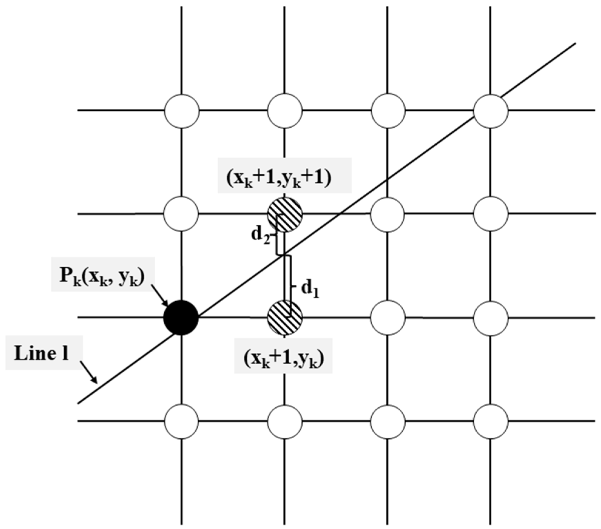
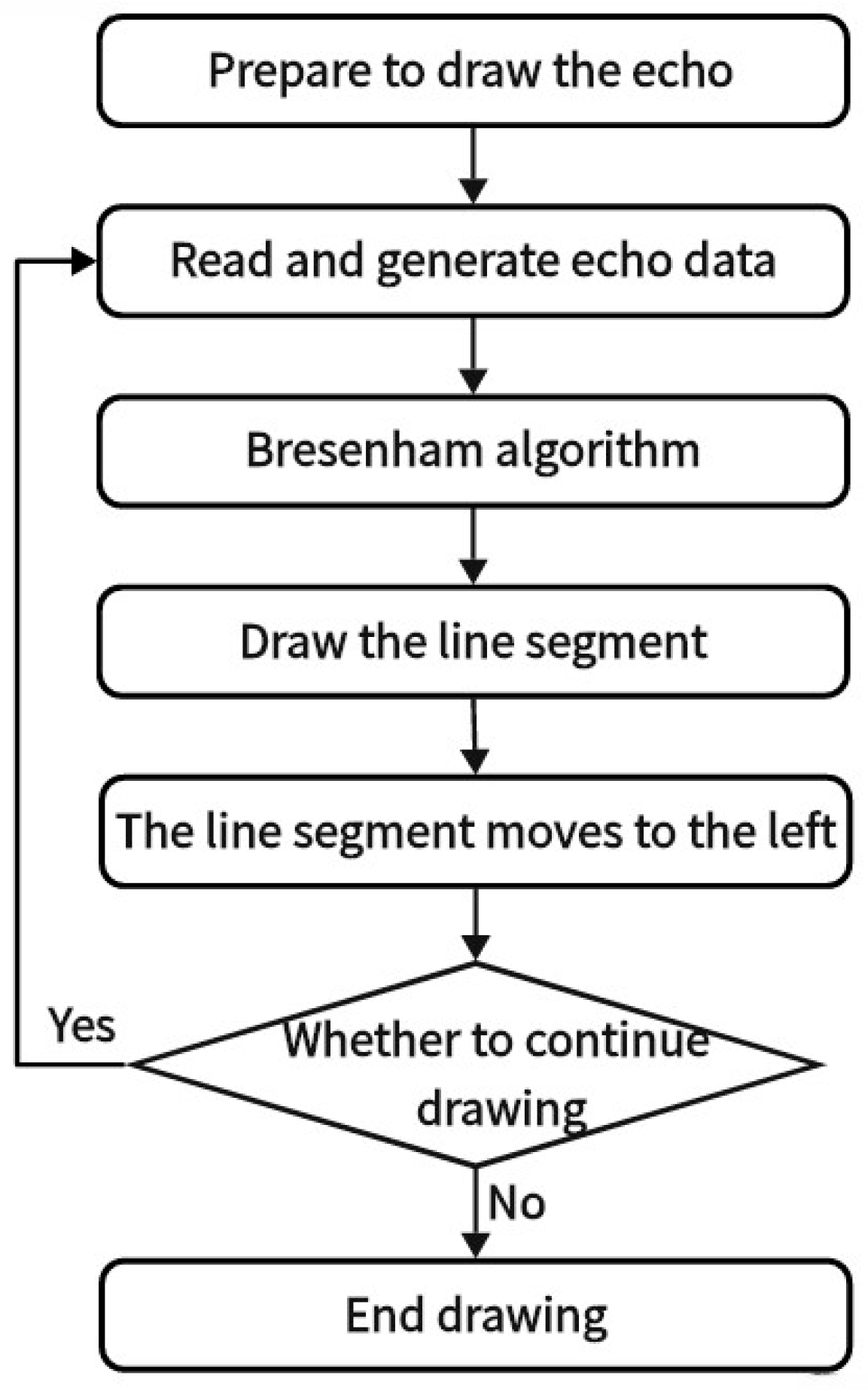
2.3. Seabed Echo Generation Algorithm

The echo image of the echo sounder is composed of a series of substrates of varying lengths, forming a three-part structure: upper, middle, and lower. Each substrate’s length falls within a fixed interval of random values, and the starting point of the lower substrate connects to the endpoint of the substrate above it. The color of the substrates’ transitions is from light to dark. In this paper, the Bresenham algorithm is employed to draw these substrates.

The Bresenham algorithm is a rasterization algorithm used in computer graphics to calculate lines, circles, and other shapes. Its basic principle involves incrementing or decrementing along the pixels of the desired graphic to achieve accurate rasterization. The key to this algorithm lies in determining the position of pixels at the baseline and making corresponding adjustments during each iteration, as illustrated in Figure 2.

Suppose the given line substrate has starting and ending points (x_s, y_s) and (x_e, y_e), forming the Line l. Let $\Delta x$, $\Delta y$ denote the horizontal and vertical offsets, respectively, and $m$ represent the slope of the line, with $0<m\le 1$. Then:

$$m={\displaystyle \frac{y2-y1}{x2-x1}}={\displaystyle \frac{\Delta y}{\Delta \mathrm{x}}}$$

(35)

Assuming that Pk(x_k, y_k) is a pixel to be displayed, it must be determined whether the next pixel P_k+1 is to be drawn at (x_k + 1, y_k) or (x_k + 1, y_k + 1). Given the equation of Line l, the y-coordinate at x_k + 1 on the line can be determined. Thus:

$$d_1-d_2=2m\left({\mathrm{x}}_k+1\right)+2b-2$$

(36)

By substituting $m$ from Equation (35) and performing some transformations, the following result is obtained:

$$p_k=2\Delta y·x_k-2\Delta x·y_k+c$$

(37)

where $p_k$ is the decision parameter in the Bresenham line-drawing algorithm at step k, and c is a constant equal to $2\Delta y+\Delta x\left(2b-1\right)$.

Based on the above, the following conclusions can be deduced:

(1)

If $p_k\le 0$(i.e., $d_1\le d_2$), then $y_{k+1}=y_k$.

(2)

If $p_k>0$(i.e., $d_1>d_2$), then $y_{k+1}=y_k+1$.

Similarly, the decision parameter $p_{k+1}$ for the (k + 1)th step can be calculated. Given that $x_{k+1}=x_k+1$, and combining this with conclusion 1, the following was obtained:

(1)

If $p_k\le 0$, then $p_{k+1}=p_k+2\Delta y$.

(2)

If $p_k>0$, then $p_{k+1}=p_k+2\Delta y-2\Delta x$.

Thus, when $0<m\le 1$ the Bresenham line-drawing algorithm proceeds as follows:

(1)

Input the two endpoints of the line substrate, storing the left endpoint in (x_s, y_s).

(2)

Store (x_s, y_s) in the frame buffer memory and draw the first point.

(3)

Calculate the initial decision parameter: $p_0=2\Delta y-\Delta x$.

(4)

Starting from $k=0$, for each x_k along the line substrate, perform the following tests:

a.

If $p_k\le 0$, the next point to draw is (x_k + 1, y_k), and $p_{k+1}=p_k+2\Delta y$.

b.

If $p_k>0$, the next point to draw is (x_k + 1, y_k + 1), and $p_{k+1}=p_k+2\Delta y-2\Delta x$.

(5)

Repeat step 4) for Δx − 1 times.

Similar logic can be applied to the case when $-1<m\le 0$. For $\left|m\right|>1$, let $\Delta x=\Delta y/m$ and $\Delta y=y_e-y_s$ to derive the algorithm.

3. Result and Discussion

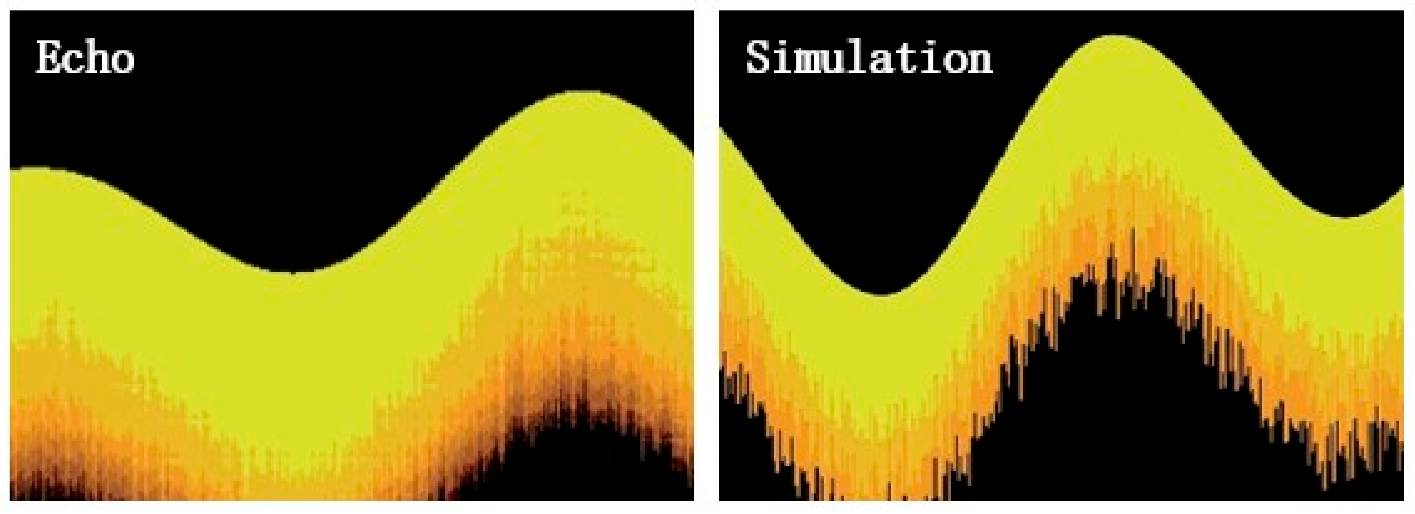
3.1. Seabed Echo Simulation

Since the upper part of the bathymetric sonar image consists of smooth curves, and the original depth data used to generate the echoes are transmitted from the electronic chart on the vessel. The density of depth points on the electronic chart is determined by factors such as the characteristics of the surveyed area, data collection density, and oceanic terrain. When the vessel is navigating along the planned route, if depth data are absent for a specific navigation point, interpolation is required between the most recent depth point and the subsequent depth point along the planned route. However, linear interpolation alone may result in a jagged effect in the upper part of the echo image, deviating significantly from the real image. Therefore, a nonlinear interpolation method is employed in this paper, utilizing the sinusoidal triangular function, which is a monotonic increasing function in the interval [0, π/2] and takes values in [0, 1]. By substituting into the following formula:

$$\sigma =\sin \left[\left(\pi ÷2n\right)\times m\right]$$

(38)

$$D=D_1+\left(D_1{-D}_2\right)\times \sigma$$

(39)

where $\sigma$ is the interpolation factor ranging from [0, 1], $n$ is the number of interpolations needed, m is the interpolation index, and $D_1$ and $D_2$ are two adjacent integers representing depths.

Thus, the depth data $D$ for the m-th interpolation can be obtained. With this formula, nonlinear interpolation echo data between two integers can be calculated, resulting in an echo image that closely resembles the real device’s image.

The echo image is divided into three substrates—upper, middle, and lower—each with a random length within a fixed interval, increasing in depth. The starting point of each lower substrate is determined by the endpoint of the substrate above it. Since the substrates in the echo image are arranged vertically and drawn from the right side of the screen, it is assumed that the horizontal distance on the screen is X and the input echo data are Y. The random values for each fixed interval substrate are denoted as R1, R2, and R3, respectively. Consequently, the starting and ending points of the upper substrate are given as (X, Y) and (X, Y + R1); the middle substrate’s starting and ending points are (X, Y + R1) and (X, Y + R1 + R2); and the lower substrate’s starting and ending points are (X, Y + R1 + R2) and (X, Y + R1 + R2 + R3). The Bresenham line-drawing algorithm is then used to draw these line substrates, resulting in a continuous echo image. The implementation process of seabed echo generation is illustrated in Figure 3.

However, the water depth data output by the echo image generated at this time do not account for the influence of the ship’s motion attitude. Considering the complex and variable sea conditions encountered by ships at sea, the vessel’s attitude can impact depth measurements. Therefore, the data transmitted by electronic charts are not the true depth data measured by the echo sounder. It is necessary to process the data to obtain the correct echo sounder depth. This study uses the roll data from the “Yu Kun” vessel of Dalian Maritime University, with the main scale parameters listed in

Table 2. Principal particulars of Yu Kun.

Items	Values
LOA (length overall)	116 m
LBP (length between perpendiculars)	105 m
B (breadth molded)	18 m
D (depth to main deck)	8.35 m
V (design speed)	16.9 kn
T (design draft)	5.4 m
GT (gross tonnage)	6106 t

. During data collection, the ship was in sea condition 4, traveling at a speed of 14.7 knots, and the sampling frequency was 1 Hz. Figure 4 shows the selected 600 s of data, and Figure 5 shows the true depth measured by the echo sounder after processing with trigonometric functions when the default electronic chart depth is 100 m. Figure 6 shows the simulated echo images with and without considering the vessel’s roll.

A series of randomly generated line substrates created using this algorithm resembles the sonar echoes from a real device, as depicted in Figure 7. From Figure 7, it can be observed that, when compared with the true machine image, the simulated image generated by the echo generation algorithm exhibits a satisfactory level of realism. The algorithm is able to effectively replicate the echo generation effects of the actual device.

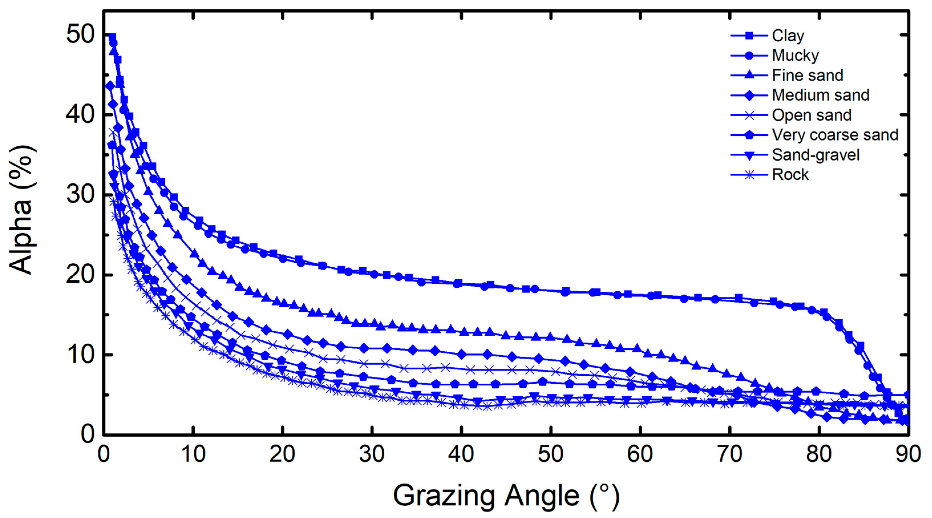
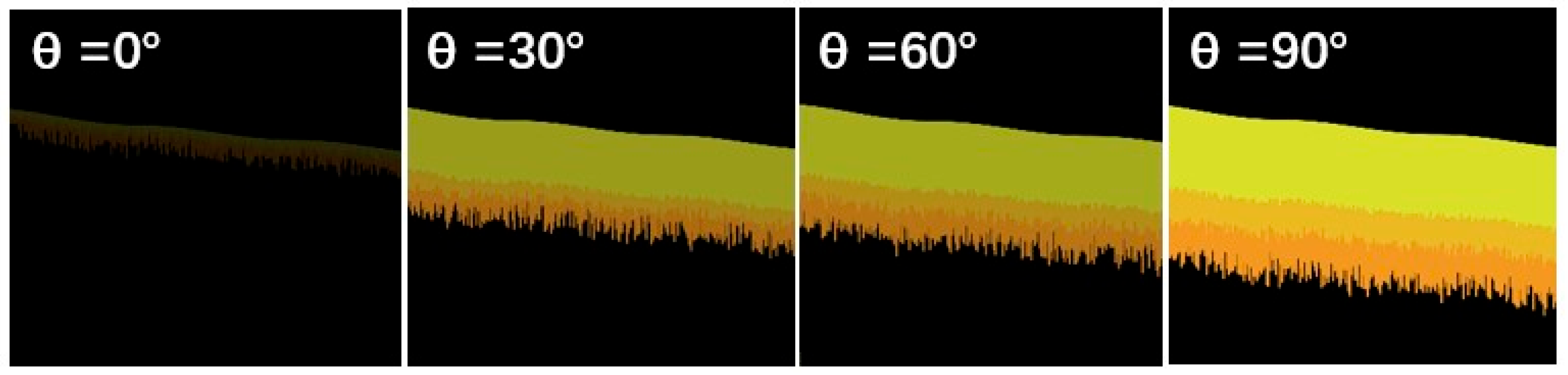
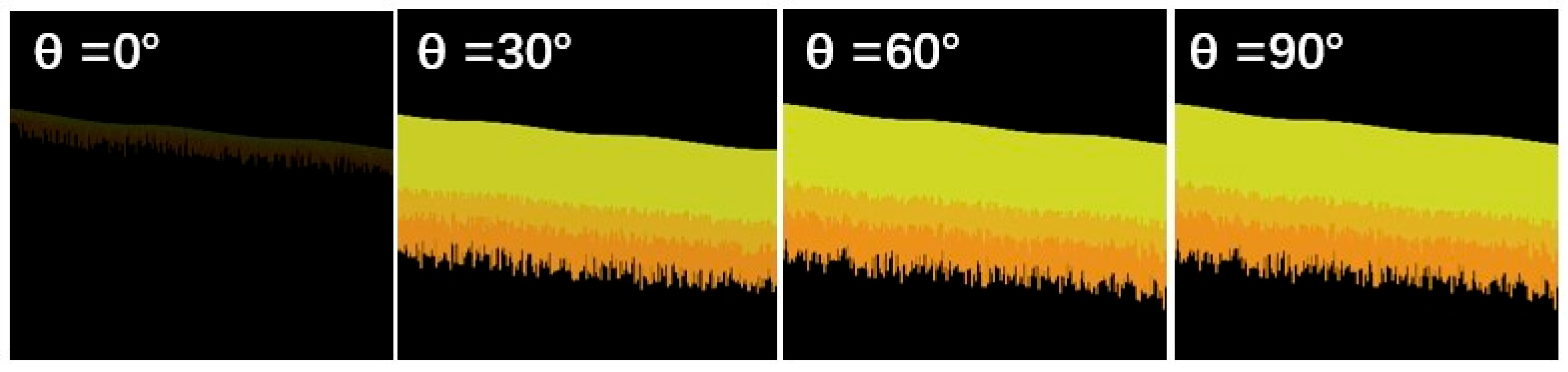
3.2. Simulation of Different Sediment Echo Intensity

The Alpha channel is a common concept in image processing, used to represent the transparency information of an image. In the RGB color space, each pixel is typically composed of three color channels: red, green, and blue. The Alpha channel is an additional channel used to store the transparency value of the pixel, usually ranging from 0 to 255 or 0% to 100%. This article introduces the concept of the Alpha channel to demonstrate variations in backscattering images of different roughness sediment by altering the transparency of the image color.

Using the empirical values of acoustic parameters for different sediment types listed in

Table 3. Empirical value of acoustic parameters.

Substrate	Average Size (mm)	Density Ratios $\mathsf{\rho }$	Sound Velocity Ratio $\mathsf{\nu }$	Parameter Losses $\mathsf{\delta }$	Volume Parameter ${\mathsf{\sigma }}_2$	Spectral Index $\mathsf{\gamma }$	Spectrum Intensity (cm4)
rock	—	2.5	2.5	0.01374	0.002	3.25	0.01862
sand–gravel	—	2.5	1.5	0.014	0.002	3.25	0.014
very coarse sand	2.0	2.492159	1.286925	0.0164595	0.002	3.25	0.01293447
open sand	1.0	2.3139	1.2278	0.01566176	0.002	3.25	0.008601511
medium sand	0.5	2.151217	1.174087	0.0157149	0.002	3.25	0.00558833
fine sand	0.25	1.615902	1.139692	0.01610051	0.002	3.25	0.0035
mucky	0.02	1.149182	0.9881798	0.005651104	0.001	3.25	5.175 × 104
clay	0.002	1.144875	0.9801043	0.0014725417	0.001	3.25	5.175 × 104

, the Jackson model is simulated, and the results are processed to obtain the backscattering color intensity variation graph as shown in Figure 8. From Figure 8, it can be observed that under the same sediment conditions, the intensity of backscattering images increases with the increase in grazing angle, especially noticeable at small grazing angles. For different sediment conditions, the curves intersect only near a grazing angle close to 90°, otherwise, they generally follow the trend that greater roughness corresponds to greater backscattering intensity.

Figure 9 and Figure 10, respectively, depict simulated backscattering images for clay and rock sediments at different grazing angles (0°/30°/60°/90° from left to right). It can be observed from the actual simulated images that, under the same seabed condition, the echo images become progressively clearer and brighter as the grazing angle increases. Under the same grazing angle, the differences in echo images between rocky and clayey seabeds are not significant only when the grazing angle is close to 90° or 0°. In other cases, the clarity of echo images from rocky seabeds is noticeably better than that from clayey ones.

Due to the acoustic beam pitch angle of the device is 60°, it can be seen from Figure 8 that the Alpha values at this angle are as shown in

Table 4. Alpha values for different seabed substrates at 60°.

Substrate	Clay	Mucky	Fine Sand	Medium Sand	Open Sand	Very Coarse Sand	Sand–Gravel	Rock
Alpha (%)	17.4	17.3	10.3	7.4	6.6	6.0	4.4	4.1

. Because the Alpha values for clay and silt are similar to those for sand–gravel and rock, when plotting backscattering images of different seabed sediments, they are divided into six categories: clay, mucky, fine sand, medium sand, open sand, very coarse sand, and rock sand–gravel. Figure 11 displays backscattering images for six different sediment conditions.

From the actual simulation comparison images, it can be determined that at a grazing angle of 60°, as the roughness of the seabed increases, the echo intensity becomes greater, and the resulting echo images are clearer and brighter. Additionally, since the echo intensities of some seabed types are close to each other, the impact of classifying them into one category is minimized, which is beneficial for the smooth operation of the system.

3.3. Simulation of Gain, Noise and Clutter

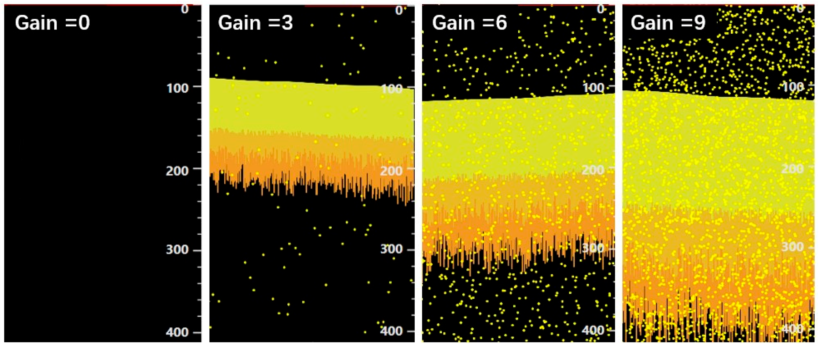
3.3.1. Gain

Adjustment of the echo sounder’s backscattering image can be achieved by changing the gain (0–9 levels), wherein the simulation involves elongating or shortening the simulated image of the echo and generating or reducing random noise dots on the screen to achieve the effect of adjusting the echo image. Figure 12 illustrates the specific simulation effects, with the backscattering images at gain levels of 0/3/6/9 from left to right.

Gain adjustment is crucial for the performance of the echo sounder. From the simulation images, it can be seen that when the gain is set too low, echo signals may be insufficiently amplified, resulting in either failure to correctly receive the echo signals or very weak echo signals. Low gain settings may lead to unstable measurements, intermittent data, or complete data loss. Conversely, when the gain is set too high, excessive amplification of the echo signals can occur, causing both noise and echo signals to be amplified. This can result in excessive noise in the received echo signals, leading to potential deviations in the actual depth measurements and inaccurate results. Therefore, gain adjustment should be guided by ensuring that echo signals are clearly discernible and that noise is minimized.

3.3.2. Noise and Clutter

Noise simulation is divided into two parts. The first part involves environmental noise, such as marine life and nearby vessels. Using the weight functions described in Section 2.2.1, various types of noise images can be generated, such as bubble noise shown in Figure 13 and noise from nearby vessels depicted in Figure 14. The second part covers reverberation noise, which follows a Rayleigh distribution and manifests as speckle noise. Clutter primarily consists of high-density biological entities like fish schools located beneath the vessel, and this can also be simulated using weight functions. Figure 15 illustrates both reverberation noise and fish school clutter.

Random noise, bubble interference, co-frequency interference, and fish school interference can significantly affect the measurement results of echo sounders. By conducting separate simulations for different types of noise, operators can be aided in more accurately identifying the type of noise and making appropriate adjustments, such as modifying the gain or adjusting the transmission frequency, to counteract its effects. Therefore, the simulation of different types of noise is deemed essential.

3.4. Echo Sounder Equipment Simulation

3.4.1. Simulation Architecture Design

The FE-800 echo sounder equipment is primarily composed of a display interface and an operation panel. To ensure consistency with the actual machine, photographs of the real device are used. These photographs undergo a series of image beautification processes and are then set as the background of a grid control. Subsequently, animation effects for the operation panel buttons, interface design, and interaction between the two parts are implemented. The simulation structure of the device is depicted in Figure 16.

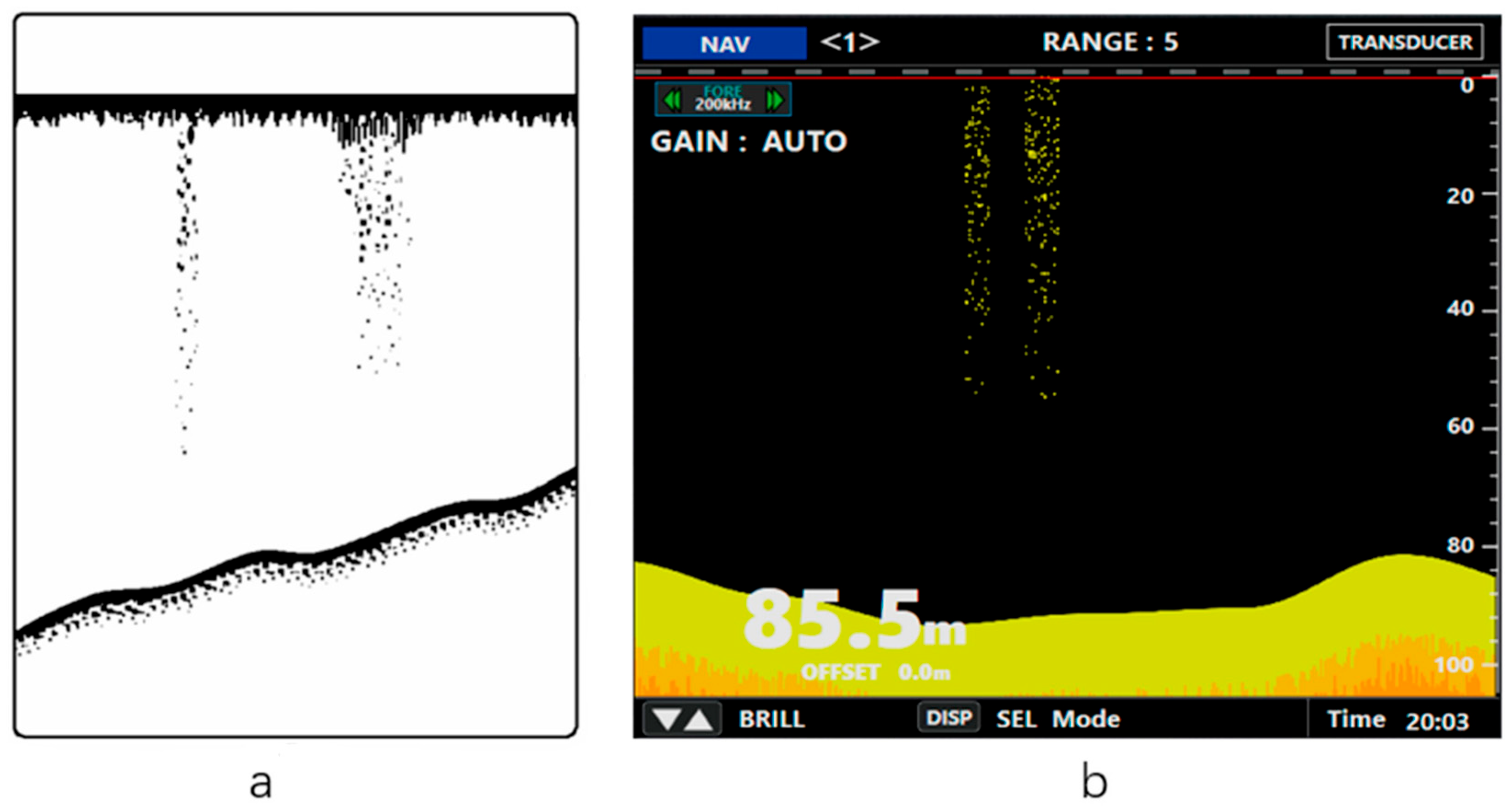
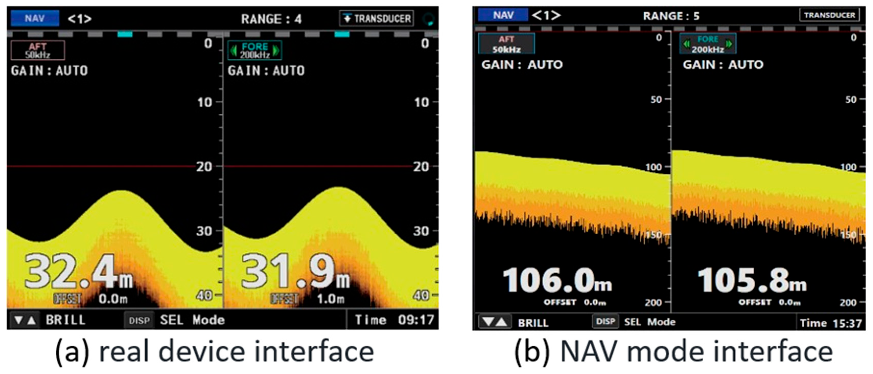
3.4.2. Simulation Effects

The simulation device for the echo sounder is designed to simulate and operate the FE-800 echo sounder produced by FURUNO on the Windows 11, Visual Studio 2022 platform. The main interface of the actual device is shown in Figure 17a, while the main interfaces of the simulated device are presented in Figure 17b–d. The LOGBOOK interface is illustrated in Figure 18a, the range adjustment is depicted in Figure 18b, the image adjustment during gain adjustment is demonstrated in Figure 18c, and the overall simulation effect is presented in Figure 18d.

4. Conclusions

This paper focuses on the simulation of echo images for shipborne echo sounders. Based on the seabed echo scattering model and noise model, a seabed echo generation algorithm was established and simulations of seabed echoes, clutter, and noise were implemented. A typical commercial ship echo sounder simulation device was developed. The main contributions of the paper are as follows:

(1)

Seabed Echo Simulation: A seabed echo rendering algorithm was proposed, which allows the simulated echoes generated by this algorithm to more accurately reproduce the echo images of actual equipment, achieving satisfactory results.

(2)

Impact of Incident Angle and Seabed Composition on Seabed Echo Simulation: Using the Jackson sound scattering model, the relationship between echo strength and incident angle for different seabed substrates was determined. Seabed echoes were rendered based on these results, producing images of seabed echoes for various seabed substrates and incident angles, visually illustrating the impact of incident angle and seabed substrate on seabed echo simulation.

(3)

Clutter and Noise Simulation: Through analysis and research on marine environmental noise and reverberation noise, the most prominent sources of noise and clutter were summarized, and their respective image simulations were conducted to enhance realism.

(4)

Simulation Equipment Development: A simulation architecture for echo sounders was designed, and a complete simulator system was developed. This system effectively realizes the main functions of an echo sounder, such as range setting, gain adjustment, operating frequency setting, and display mode switching. The simulation visuals and operational realism closely approach that of actual equipment.

The simulated seabed echoes and clutter show good realism, and the developed simulation device is functionally complete, meeting the requirements of the STCW 2010 international convention and suitable for echo sounder operation training for maritime personnel.

References

1. Jin, Y.; Yin, Y. The Development Strategy of Marine Simulators under the Manila Amendment to the STCW Convention. Navig. China 2012, 35, 5–10. [Google Scholar]
2. Yang, X.; Ren, H.; Lian, J.; Wang, D. VR interactive 3D virtual ship modeling and simulation. Navig. China 2022, 45, 37–42+49. [Google Scholar]
3. Maritime Safety Administration of the People’s Republic of China. The Manila Amendment to the International Convention on Standards of Training, Certification and Watchkeeping for Seafarers, 1978; Dalian Maritime University Press: Dalian, China, 2010. [Google Scholar]
4. Yang, C.; He, Q. Application and Prospect of Intelligent Ship. Sci. Technol. Innov. 2023, 75–77. [Google Scholar] [CrossRef]
5. Jackson, D.R.; Baird, A.M.; Crisp, J.J.; Thomson, P.A.G. High-frequency bottom backscatter measurements in shallow water. J. Acoust. Soc. Am. 1986, 80, 1188–1199. [Google Scholar] [CrossRef]
6. Jackson, D.R.; Briggs, K.B. High-frequency bottom backscattering: Roughness versus sediment volume scattering. J. Acoust. Soc. Am. 1992, 92, 962–977. [Google Scholar] [CrossRef]
7. Zheng, Y.; Qin, Z.; Yu, S.; Ma, B.; Zhao, J.; Liu, M. Progress and Prospect of Seabed Acoustic Scattering Characteristics. J. Harbin Eng. Univ. 2024, 45, 748–757. [Google Scholar]
8. Peng, Z.; Zhou, J.; Zhang, R. In-plane seabed scattering caused by inhomogeneous seabed and rough interface. Sci. Sin. (Phys. Mech. Astron.) 2004, 34, 378–391. [Google Scholar]
9. Jackson, D.R.; Odom, R.I.; Boyd, M.L.; Ivakin, A.N. A geoacoustic bottom interaction model (GABIM). IEEE J. Ocean. Eng. 2010, 35, 603–617. [Google Scholar] [CrossRef]
10. Weidner, E.; Weber, T.C. An acoustic scattering model for stratification interfaces. J. Acoust. Soc. Am. 2021, 150, 4353–4361. [Google Scholar] [CrossRef]
11. Zhang, S.; Wu, J.; Yin, T. Simulation of sonar reverberation signal considering the ocean multipath and Doppler effect. Front. Mar. Sci. 2023, 10. [Google Scholar] [CrossRef]
12. Thorsos, E.I.; Williams, K.L.; Chotiros, N.P.; Christoff, J.T.; Commander, K.W.; Greenlaw, C.F.; Holliday, D.V.; Jackson, D.R.; Lopes, J.L.; McGehee, D.E.; et al. An overview of SAX99: Acoustic measurements. IEEE J. Ocean. Eng. 2001, 26, 4–25. [Google Scholar] [CrossRef]
13. Holland, C.W. Coupled scattering and reflection measurements in shallow water. IEEE J. Ocean. Eng. 2002, 27, 454–470. [Google Scholar] [CrossRef]
14. Yang, Y. Study of high frequency seabed scattering based on Jackson model. Acoust. Electron. Eng. 2015, 33–36. [Google Scholar]
15. Ohkawa, K.; Yamaoka, H.; Yamamoto, T. Acoustic backscattering from a sandy seabed. IEEE J. Ocean. Eng. 2005, 30, 700–708. [Google Scholar] [CrossRef]
16. Yu, S.; Liu, B.; Yu, K.; Yang, Z.; Kan, G.; Zhang, X. Comparison of acoustic backscattering from a sand and a mud bottom in the South Yellow Sea of China. Ocean Eng. 2020, 202, 107145. [Google Scholar] [CrossRef]
17. Zheng, P.; Zhang, H.; Pan, Z.; Qian, H. Imaging simulation and range analysis of multi-beam bathymetric sonar. Digit. Ocean Underw. Warf. 2023, 6, 664–669. [Google Scholar] [CrossRef]
18. Jiang, N. Research on Simulation Testing Method of the Doppler Velocity Sonar. Master’s Thesis, Harbin Engineering University, Harbin, China, 2017. [Google Scholar]
19. Ding, Y. Research on Echo Simulation and Image Generation Technology of Seabed Objects. Master’s Thesis, Northwestern Polytechnical University, Xi’an, China, 2006. [Google Scholar]
20. Chen, D.; Ren, H.; Yin, J. Design and realization on simulation software of Echo sounder. Inf. Technol. J. 2013, 12, 3645–3649. [Google Scholar] [CrossRef]
21. Zhou, J. Research on Virtual Echo Sounder Based on LabVIEW. Master’s Thesis, Huaqiao University, Quanzhou, China, 2015. [Google Scholar]
22. Hou, C.; Li, H.; Wang, L.; Zhang, S. Research on virtual echo sounder based on LabVIEW. Comput. Program. Ski. Maint. 2015, 81+93. [Google Scholar] [CrossRef]
23. Jackson, D.R.; Richardson, M.D. High-Frequency Seafloor Acoustics; Springer: New York, NY, USA, 2007. [Google Scholar]
24. Zou, B. Study on Seafloor Sediment Parameter Inversion Based on Acoustic Backscattering Model. Ph.D. Thesis, Tianjin University, Tianjin, China, 2020. [Google Scholar]
25. Zhou, J. Research on Denoising Method of Underwater Acoustic Image. Master’s Thesis, University of Electronic Science and Technology of China, Chengdu, China, 2019. [Google Scholar]
26. Siano, D.; González, A.E. Noise and Environments; IntechOpen: London, UK, 2021. [Google Scholar] [CrossRef]
27. Wenz, G.M. Acoustic Ambient Noise in the Ocean: Spectra and Sources. J. Acoust. Soc. Am. 1962, 34, 1936–1956. [Google Scholar] [CrossRef]
28. Liu, B.; Huang, Y.; Chen, W.; Lei, J. Principles of Underwater Acoustics, 3rd ed.; Science Press: Beijing, China, 2019. [Google Scholar]
29. Zhang, H.; Cheng, J.; Tian, M.; Liu, J.; Shao, G.; Shao, S. A Reverberation Noise Suppression Method of Sonar Image Based on Shearlet Transform. IEEE Sens. J. 2023, 23, 2672–2683. [Google Scholar] [CrossRef]
30. Liu, G.; Liu, B.; Hu, J.; Cang, Y.; Zhao, N.; Zhou, B. Sonar image denoising in NSCT domain based on neutral set and bilateral filtering. J. Hunan Univ. (Nat. Sci.) 2023, 50, 19–27. [Google Scholar] [CrossRef]
Figure 1. The schematic diagram of seabed acoustic scattering.
Jmse 12 01762 g001
Figure 2. Bresenham algorithm.
Jmse 12 01762 g002
Figure 3. Process of seabed echo generation.
Jmse 12 01762 g003
Figure 4. Ship rolling data.
Jmse 12 01762 g004
Figure 5. Sounder depth in roll attitude.
Jmse 12 01762 g005
Figure 6. Simulated echo images for ship stationary and roll conditions.
Jmse 12 01762 g006
Figure 7. Simulation result of the seabed echo image.
Jmse 12 01762 g007
Figure 8. The curve of echo intensity change.
Jmse 12 01762 g008
Figure 9. Echo images of different grazing angles under clay substrate.
Jmse 12 01762 g009
Figure 10. Echo images of different grazing angles under rock substrate.
Jmse 12 01762 g010
Figure 11. Different sediment echo images.
Jmse 12 01762 g011
Figure 12. The effect of echo image under different gain.
Jmse 12 01762 g012
Figure 13. Bubble noise; (a) real equipment; (b) simulation image.
Jmse 12 01762 g013
Figure 14. Interference noise from other ships: (a) real equipment; (b) simulation image.
Jmse 12 01762 g014
Figure 15. Reverberation noise and fish school clutter.
Jmse 12 01762 g015
Figure 16. Simulation structure diagram of echo sounder device.
Jmse 12 01762 g016
Figure 17. Simulation effect of main interface.
Jmse 12 01762 g017aJmse 12 01762 g017b
Figure 18. Simulation effect of function implementation.
Jmse 12 01762 g018