Abstract
A novel Boundary Element Method (BEM) is presented for predicting the hydrodynamic behavior of twin-hull vessels, traveling at low speeds, aiming to quantify the benefits of integrating solar technology onboard. In particular, the power requirements of an electric 33 m long twin-hull ship are examined. The study discusses the placement of solar panels on deck and assesses their utilization in terms of real-time energy generation, aiming to extend the autonomy range while also reducing carbon emissions. The discussed methodology predicts the power needs by considering various operational variables, design specifications and hydrodynamic principles. In addition, it addresses the viability and possible advantages of integrating solar technology onboard and provides preliminary estimates regarding the extent to which solar energy may compensate for power needs, based on several factors, including the velocity, the prevailing sea state and the incident solar irradiance. The results provide useful information regarding the utilization of solar energy in the shipping sector, in addition to advancing sustainable maritime propulsion.
1. Introduction
In recent years, the maritime industry has been increasingly exploring sustainable alternatives to traditional fossil fuel-powered propulsion systems, driven by concerns over environmental impact as well as rising fuel costs. A promising path is the integration of solar power into ship design, offering a renewable and environmentally friendly source of energy. This has led interest in solar-powered vessels to grow, as they offer a solution to the demand for environmentally friendly maritime transportation, while simultaneously providing several other key benefits. The latter include independence from fossil fuels, lower noise levels, and reduced maintenance costs [1]. Furthermore, solar-powered vessels provide enhanced safety by minimizing fuel-related risks [2].
The potential benefits of integrating solar technology for covering the hotel loads of recreational boats are discussed in ref. [3]. Moreover, ref. [4] provides financial and technical analyses of solar vessels, including estimated investment costs. The latter work also concludes that a sufficient energy storage system is required, as the real-time solar power generated is inadequate for achieving sufficient propulsion speed. Meeting the total energy demands of a vessel solely through solar power is a challenging objective, given the current technological constraints. However, there are research studies that address this concept, particularly focusing on catamaran vessels operating at low speeds (see e.g., ref. [5]). This approach seeks to maximize the available surface area for photovoltaic (PV) array installations while simultaneously minimizing resistance. Standalone PV-based systems for small ships are also discussed in ref. [6].
This paper focuses on assessing the feasibility and potential benefits of integrating solar panels onboard a 33 m twin-hull vessel operating in the Greek seas. Greece, having an extensive coastline and abundant incidence of solar irradiance almost throughout the whole year (see e.g., ref. [7]), presents a promising environment for the implementation of solar-powered maritime solutions. Based on a case study approach, this work aims to assess the efficacy of integrating solar energy systems in short-haul maritime operations and to quantify the extent to which solar power can offset the vessel’s total energy requirements by combining data from hydrodynamic analysis with a photovoltaic (PV) model. The assessment of solar panel integration for partially covering the energy needs of the vessel requires a comprehensive analysis of the latter’s resistance components, as well as an estimate of the energy required for service loads (lighting, navigation equipment, communication systems). For the scope of this work, considering low operational speeds, the appendage and air resistance components are excluded from the analysis, and the calm water resistance is approximated by the wave-making and the frictional resistance components. The wave-making resistance is calculated by a Boundary Element Method (BEM), which evaluates the resulting Kelvin pattern generated by the vessel’s forward motion. The stationary nature of the generated wave pattern, as observed from a body-fixed reference frame onboard the vessel, allows for the calculation of the corresponding flow field without necessitating time-dependency considerations. It is important to note that the BEM approach relies on linear theory, which implies that flow rotation, compressibility and viscosity are not considered. However, the simplified model still provides valuable insights into the hydrodynamic behavior of the vessel, as regards wave generation and resistance at Froude numbers corresponding to velocities well below the hull speed, where the vessel primarily operates as a displacement craft. The frictional resistance component is incorporated based on the International Towing Tank Conference (ITTC) 1957 recommendations [8]. Moreover, an additional hydrodynamic model is developed and employed to evaluate the Response Amplitude Operators (RAOs) of the vessel under harmonic wave excitation, depending on the prevailing sea conditions, assuming harmonic time dependence of the whole hydromechanical system. By considering the total wave field generated by the vessel’s interaction with an incident field at a given velocity, the added wave resistance is also evaluated. The above approach allows for a thorough examination of the vessel’s performance and power requirements under different sea states, laying the groundwork for assessing the feasibility and efficacy of solar panel integration for propulsion in Greek maritime operations. The discussed BEM formulation involves a steady and an unsteady model, both of which are combined with a four-point upstream finite difference scheme, to treat the combined effect of incident flow and waves interacting with the twin-hull vessel, supporting an accurate calculation of the total resistance (including the added resistance component), as well as the responses. Moreover, the steady model employs a mirroring technique while the unsteady one is supplemented by a Perfectly Matched Layer (PML) technique, as discussed in detail in the sequel.
The available solar power is derived using a simple photovoltaic (PV) model, which utilizes data provided by the SARAH2 database [https://joint-research-centre.ec.europa.eu/photovoltaic-geographical-information-system-pvgis/pvgis-data-download/sarah-2-solar-radiation-data_en (accessed on 16 July 2024)], which offers information on solar irradiance levels among other parameters, enabling the estimation of the available solar energy potential. The PV model utilizes data of the vessel’s responses in the rotational degrees of freedom to simulate instantaneous angular changes in the panels mounted on deck and accurately account for the variations in solar exposure experienced by the integrated solar system. By coupling these data with the energy requirements and the resistance components discussed earlier, this work aims to provide a holistic assessment of the feasibility and effectiveness of solar panel integration for sustainable maritime operations. This interdisciplinary approach combines principles from various fields, including naval architecture, renewable energy and solar technology, to address the complex challenges of transitioning towards greener maritime transportation solutions.
2. Problem Formulation
The geometry of the twin-hull vessel studied in the context of the present work is based on optimized results from the literature. In particular, the dimensions and hull lines of each demi-hull are used as parametrically optimized by Kanellopoulou et al. [9], in the framework of the ELCAT research project [https://elcatproject.gr/ (accessed on 5 July 2024)]. The latter project, conducted from 2020 to 2023, was a collaboration between NTUA (National Technical University of Athens) and Alpha Marine, focusing on designing energy-efficient electric catamarans, measuring between 19 m and 33 m in length. The project’s aim was to contribute to a reduction in greenhouse gas emissions and atmospheric pollution from the shipping industry. The primary design configuration employed is that of the 33 m long vessel developed within the aforementioned project and the configuration of the solar panels deployed on deck is adapted to the specific features of this vessel (see Figure 1).
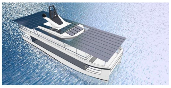
Figure 1.
Illustration of the 33 m long twin-hull vessel with integrated solar panels.
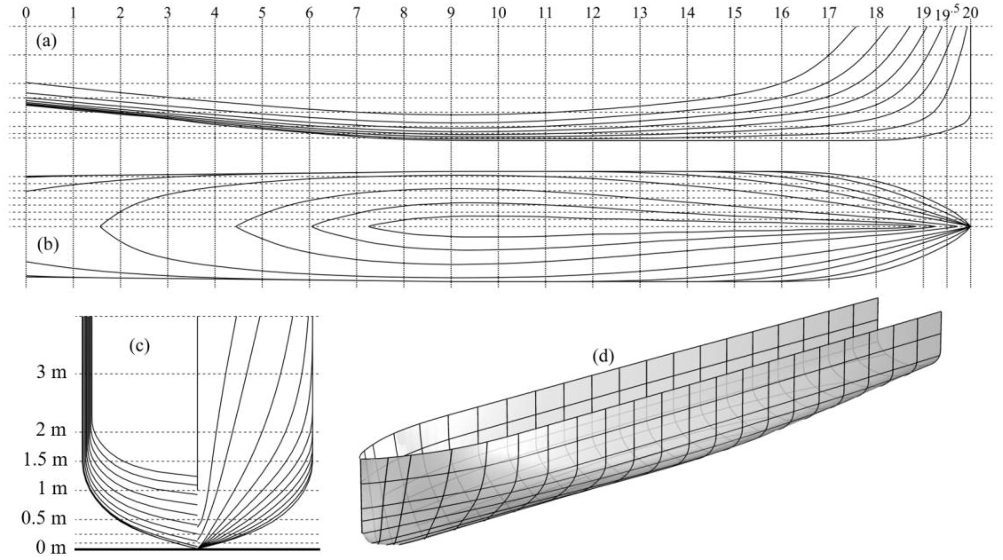
The hull lines are illustrated in Figure 2a–c, along with a 3D view of the demi-hull (Figure 2d) that offers a more detailed perspective of the demi-hull’s shape. Indicative waterline levels are also depicted in the body plan (Figure 2c) for various drafts, facilitating the visualization of the submerged geometry at different loading conditions. The main characteristics of the vessel are listed in Table 1.

Figure 2.
Lines plan of the demi-hull form (a) sheer plan, (b) breadth plan (waterlines), (c) body plan, and indicative waterline levels; (d) 3D view, incorporating the breadth and body plan lines in 3D space.

Table 1.
Main parameters of the fully electric version of the twin-hull vessel [source: https://elcatproject.gr/ (accessed on 5 July 2024)].
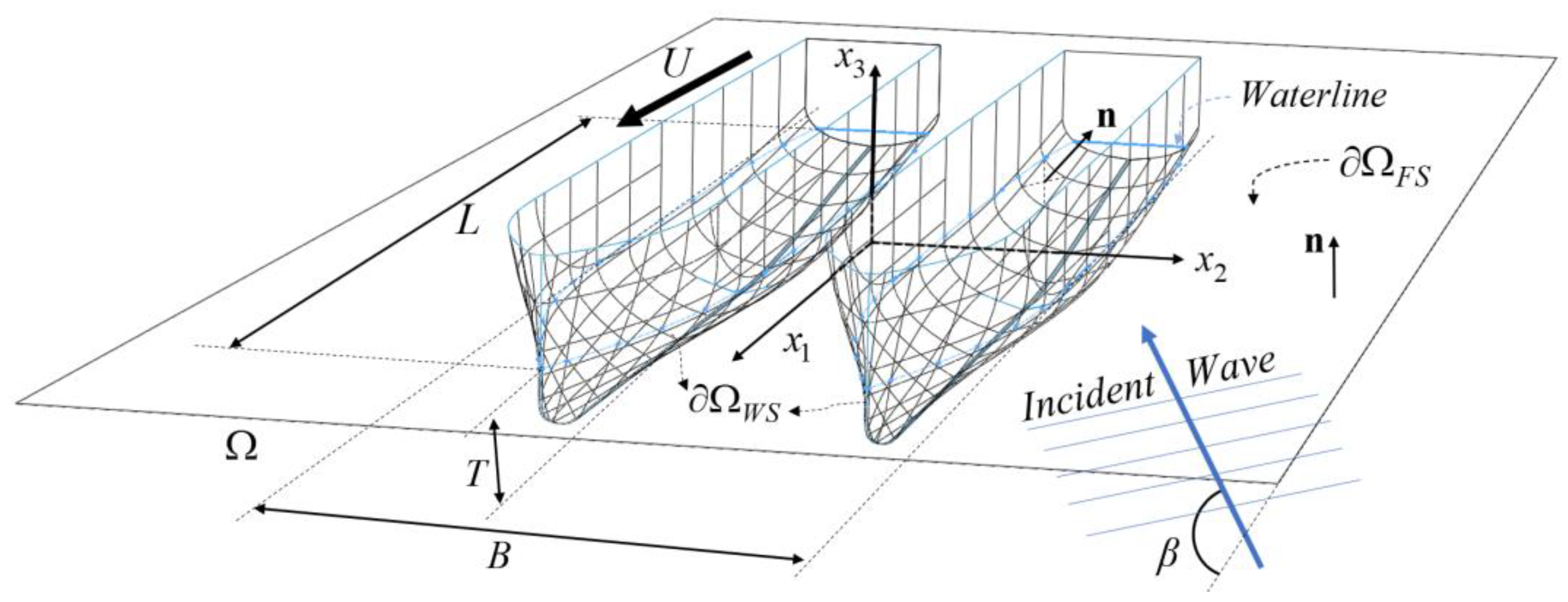
The coordinate system is used, with the origin placed at Mean Water Level , coinciding with the center of flotation. The -axis runs parallel to the vessel’s length, is the transverse axis, and the vertical coordinate is negative in the water body. Let denote a flow domain that extends infinitely to all azimuthal directions as well as the negative -direction, and is bounded by the free surface of the water at and the wetted surface of the twin hull. In the body-fixed coordinate system , the forward motion of the vessel at speed along the -direction translates to the existence of a uniform water flow moving at constant speed opposite to this direction.
The dynamic behavior of the vessel is analyzed in the framework of linear wave theory, enabling the flow variables to be decomposed into a steady background flow and a time-dependent wave component, which is treated as harmonic. The velocity fields of the total flow components are described by the gradients of appropriate potential functions defined in .
Given the stationary nature of both the uniform flow and the generated Kelvin pattern, as observed from the body-fixed reference frame onboard the vessel, the result of the ship’s forward motion in calm water is described by steady (time-independent) potential functions, namely, the steady incident field (uniform flow) and a perturbation field, generated by the interaction of the wetted surface and the uniform water flow of velocity . The unsteady, time-dependent (wave) problem presents more complexity since the analysis involves an incident, a diffracted, and—provided that the body is considered nondeformable—six radiated flow fields. The latter are a consequence of the vessel’s motions in six Degrees of Freedom (DoFs), which include surge, sway, heave, roll, pitch and yaw. A sketch of the studied configuration is depicted in Figure 3.
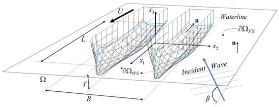
Figure 3.
Sketch of the considered hydrodynamic model, illustrating the flow domain and its boundary parts along with basic dimensions and parameters.
On the basis of linear theory, each of these motions induces a distinct outgoing (radiated) wave field that contributes to the unsteady hydrodynamic responses. In this work’s context, is employed to denote potential functions of time-dependent flows, while (lowercase) is utilized to represent the potential of time-independent flows, ensuring clear differentiation between the two. Furthermore, potential functions involved in the steady problem are annotated with the superscript , whereas the superscript is used for potential functions corresponding to the wave problem. This serves to amplify the distinction between the two problems, since time-independent (complex) potential functions are also used for the wave problem, exploiting the assumption of harmonic time dependence, as explained in greater detail in the sequel.
2.1. Formulation of the Steady Problem
The steady flow is defined by the interaction of a uniform parallel flow directed towards the negative -axis, with the wetted surface in the domain (see Figure 3). The perturbation field is calculated following a Neumann–Kelvin (NK) formulation (see, e.g., ref. [10]) using the decomposition,
The potential function is used to describe the generated Kelvin pattern and is expected to exhibit wave-like behavior downstream. The latter function is obtained as solution to the Laplace equation, supplemented by the free-surface boundary condition and an impermeability condition at the wetted surface. Considering the transom stern geometry of the studied vessel, a false body model is adopted (see e.g., ref. [11]) to ensure that the flow separates smoothly from the hull’s surface at the aft end. This approach is based on the addition of a virtual appendage (false body—FB) to the transom. The latter encloses the separated flow at low speeds, or the created air cavity in the higher speed range [12], and excludes this region from the water body simulated by the potential flow solver. The false body naturally extends the hull geometry, initiating tangentially from the entire stern profile, ensuring a smooth geometry and thereby maintaining the integrity of the flow at the aft end of the vessel. This approach presumes the transom remains fully ventilated at all speeds, leading to transom stern drag, attributed to the absence of hydrostatic pressure on the stern, to be overestimated at low speeds [13]. The false body length is set to , where is the transverse wavelength of the Kelvin pattern. However, in cases where exceeds , being the stern beam at mean water level (MWL), the virtual appendage length is limited to . This restriction is based on experimental data provided in ref. [14], where it is shown that the boundary layer typically reattaches at a distance equivalent to six times the step height for high Reynolds number turbulent flows. Nonetheless, relevant calculations indicated that the evaluated wave-making resistance is not severely affected by this length, regardless of the precise value within these limits.
Considering the addition of the virtual boundary , the potential function is evaluated as a solution to the following BVP,
supplemented by appropriate conditions at infinity. In the above equations, represents the unit vector, normal to the boundary , pointing outward from the water body, as also shown in Figure 3. For the treatment of the above BVP, a low-order panel method is adopted using a simple singularity (source) distribution on (see, e.g., ref. [15]), in conjunction with an integral representation of . Exploiting the inherent symmetry of the discussed (steady) problem with respect to the plane , the following integral representation is utilized, which makes use of a mirroring technique to amplify computational efficiency,
The Green’s function of the Laplace equation in 3D, described by Equation (7), involves the mirror point of with respect to the symmetry plane: and is a source/sink strength distribution, defined on . The above technique introduces an artificial boundary at the symmetry plane, where a homogeneous Neumann BC is intrinsically satisfied due to the Green’s function being used. The above formulation is combined with an appropriate scheme to satisfy the conditions at infinity based on the discrete Dawson operator, as described in the sequel.
2.2. Three-Dimensional BEM for the Steady-Flow Problem
The geometry of the different sections of is approximated using 4-node quadrilateral elements, on which the strength of the singularity distribution is considered piecewise constant. In the discrete model, the field equation is inherently satisfied by the superposition of the fundamental fields generated by all elements, while the boundary conditions are satisfied at the centroid of each panel (collocation points). The induced potential and velocities associated with the -element’s contribution to the -collocation point are numerically calculated, and the corresponding matrices of induced potential ( and velocity , respectively, are computed. The latter square matrices have dimension , where , , and respectively, represent the number of quadrilateral elements distributed on the parts of corresponding to the free surface and the actual wetted surface and the false wetted surface, ensuring global continuity of geometry approximation. Consequently, the BVP is reduced to the algebraic system,
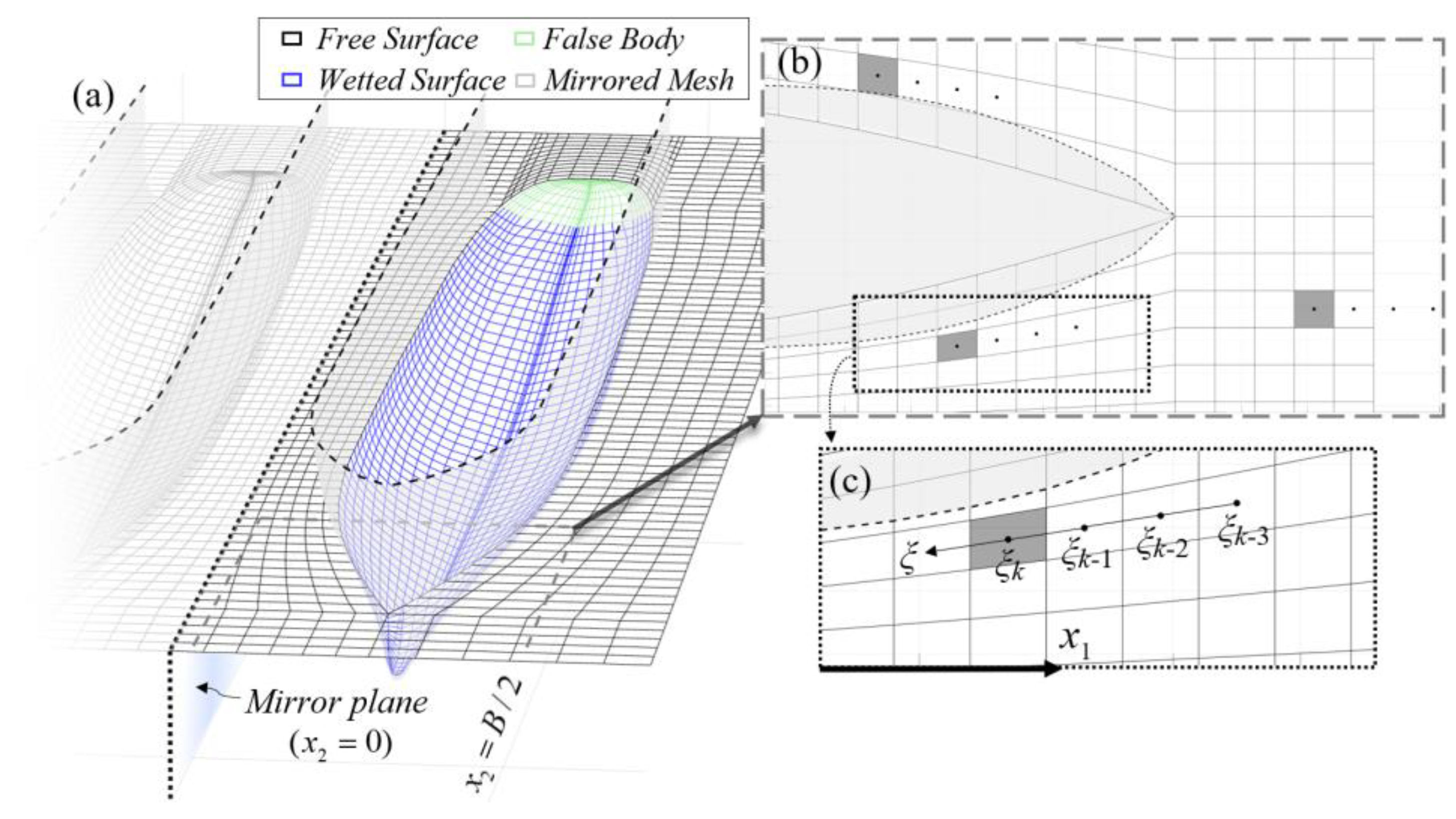
whose solution provides the strength of the source/sink distribution on each element. The latter, in conjunction with Equation (5), fully describes the resulting function in , while for it holds that . The numerical scheme involves a streamline-like arrangement of the boundary elements on , as shown in Figure 4. The acceleration in the -direction, which is involved in the free surface boundary condition [Equation (3)], is approximated by the derivative of the velocity in the -direction, as depicted in the details shown in Figure 4b,c.
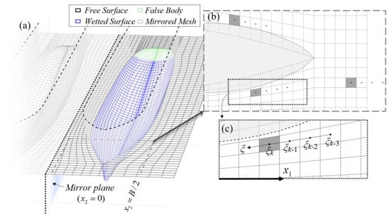
Figure 4.
(a) Indicative mesh of , illustrating a sparse discretization of the various boundary parts, along with the mirror plane. (b,c) Detailed view of the mesh at the bow, also illustrating the sets of points used in the finite difference (FD) scheme for the calculation of acceleration at indicative elements that appear shaded.
The present model involves a four-point upstream finite difference (FD) scheme based on the Dawson backward operator [16], which is defined as follows:
where
In the above equations, denotes the distance covered in a curve defined in the -direction, measured from an arbitrary point, and the velocities involved in Equation (10) are equal to
Figure 4 depicts an indicative sparse boundary mesh, where it can be seen that additional grid lines are introduced behind the stern to minimize the deviation between the differentiation direction and the actual -direction. Semicosine spacing is employed to discretize the wetted surface in the -direction to achieve increased grid resolution at the keel, where the geometry exhibits the highest gradient. Furthermore, ghost nodes are employed to assess the induced acceleration at the first three element rows of the grid (see Figure 4b). The value of the induced velocity at the ghost nodes is taken to be equal to the velocity induced at the centroid of the last actual element involved in the differentiation. The same technique is also applied to compute the acceleration at the first three element rows behind the false body mesh.
Based on the above finite difference scheme, the (non-square) matrix of dimensions is defined. The elements of this matrix,
model the contribution of the -element on at the -collocation point on the free surface. Consequently, the discrete model of the steady-flow problem, modeling the disturbance field, is defined by the linear algebraic system of Equation (8), where
After obtaining the solution to the above linear system, the free surface elevation can be obtained from the dynamic boundary condition as
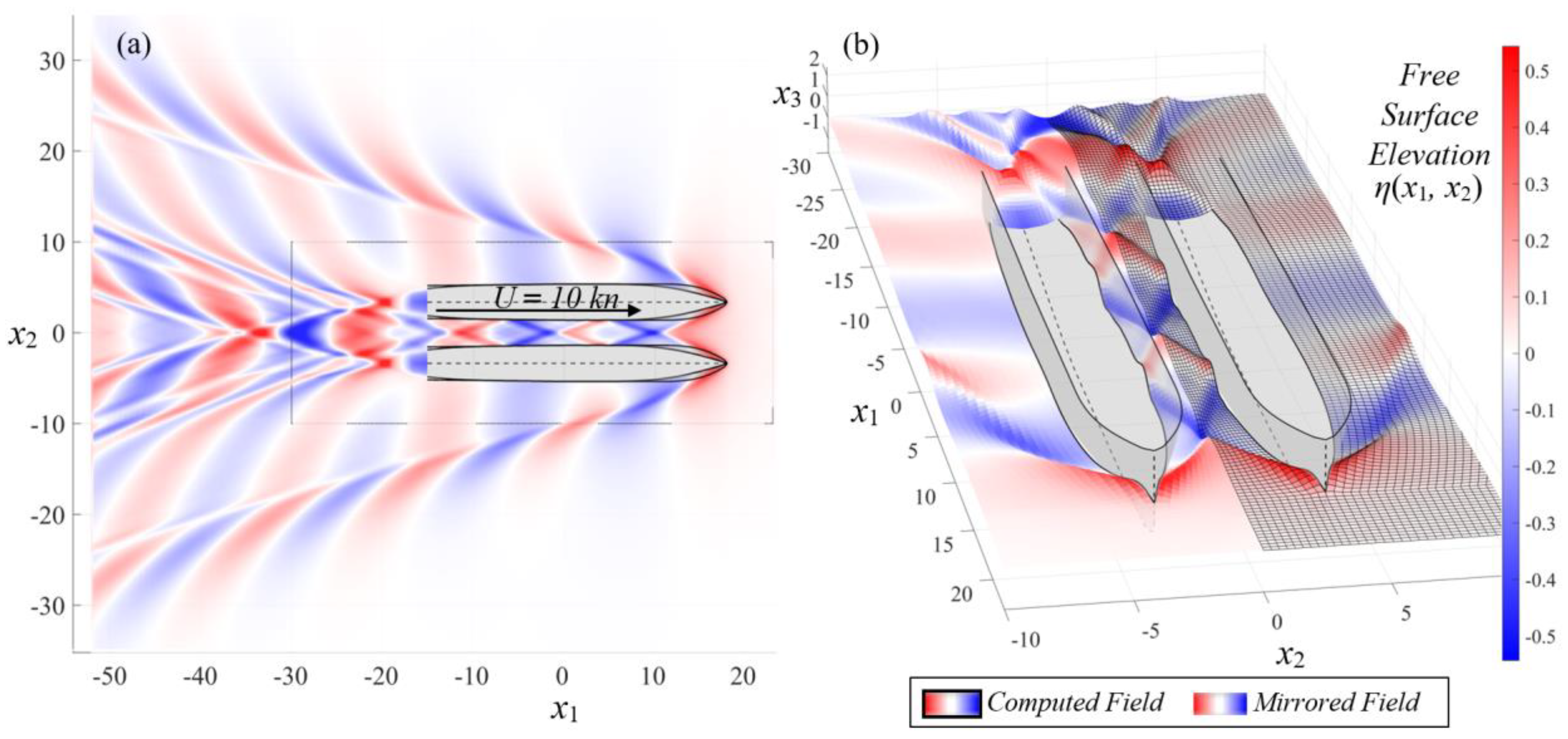
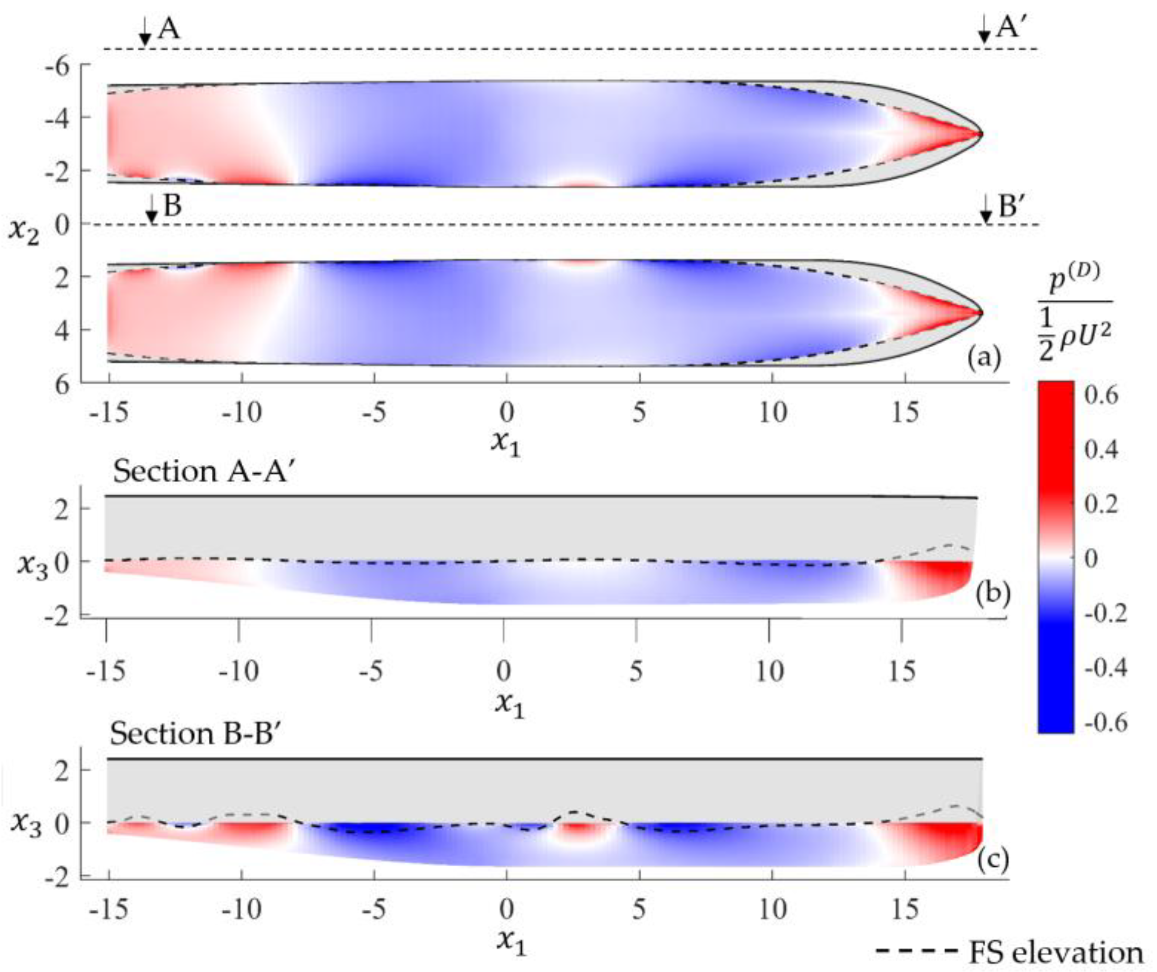
An indicative result of the field generated by the vessel moving at 10 knots is shown in Figure 5. Specifically, Figure 5a illustrates the wave-like behavior of the steady perturbation field trailing behind the vessel, demonstrating the characteristic wake pattern, and Figure 5b provides a detailed view of the solution on the computational grid in a localized area around the ship, also highlighting the directly computed solution and its mirrored counterpart. The resulting dynamic pressure on the wetted surface for the same velocity is shown in Figure 6, illustrating the pressure distribution along the hull.
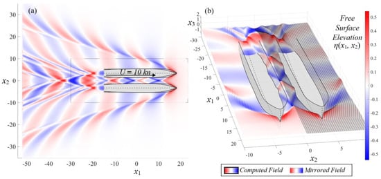
Figure 5.
Kelvin wave pattern generated by the twin-hull vessel at : (a) Top view and (b) 3D view highlighting the computed and mirrored parts of the field.

Figure 6.
Dynamic pressure distribution on the twin hull, for (a) Top view, (b) outer part of the demi-hull, and (c) inner part of the demi-hull.
The results refer to a draft of , ensuring the availability of experimental data for verification purposes. The latter data concerning calm water resistance can be found in ref. [9].
The total calm water resistance is approximated by the sum of the wave-making resistance and the frictional resistance,
where and respectively, denote the wave-making and frictional resistance coefficients, is a form factor and is the wetted surface area. The coefficient is computed using data by the steady BEM model discussed earlier. In particular, equals
where
The frictional resistance coefficient is evaluated using the ITTC 1957 formula [8],
and is scaled by the form factor which depends on the hull form and, in the case of a twin-hull configuration, can be approximated by the following equation based on the demi-hull’s slenderness ratio [17],
where denotes the submerged volume of a single demi-hull. For the considered twin-hull geometry and draft the form factor equals . The Reynolds number is evaluated, considering the dynamic viscosity of seawater at temperature T = 20 °C, .
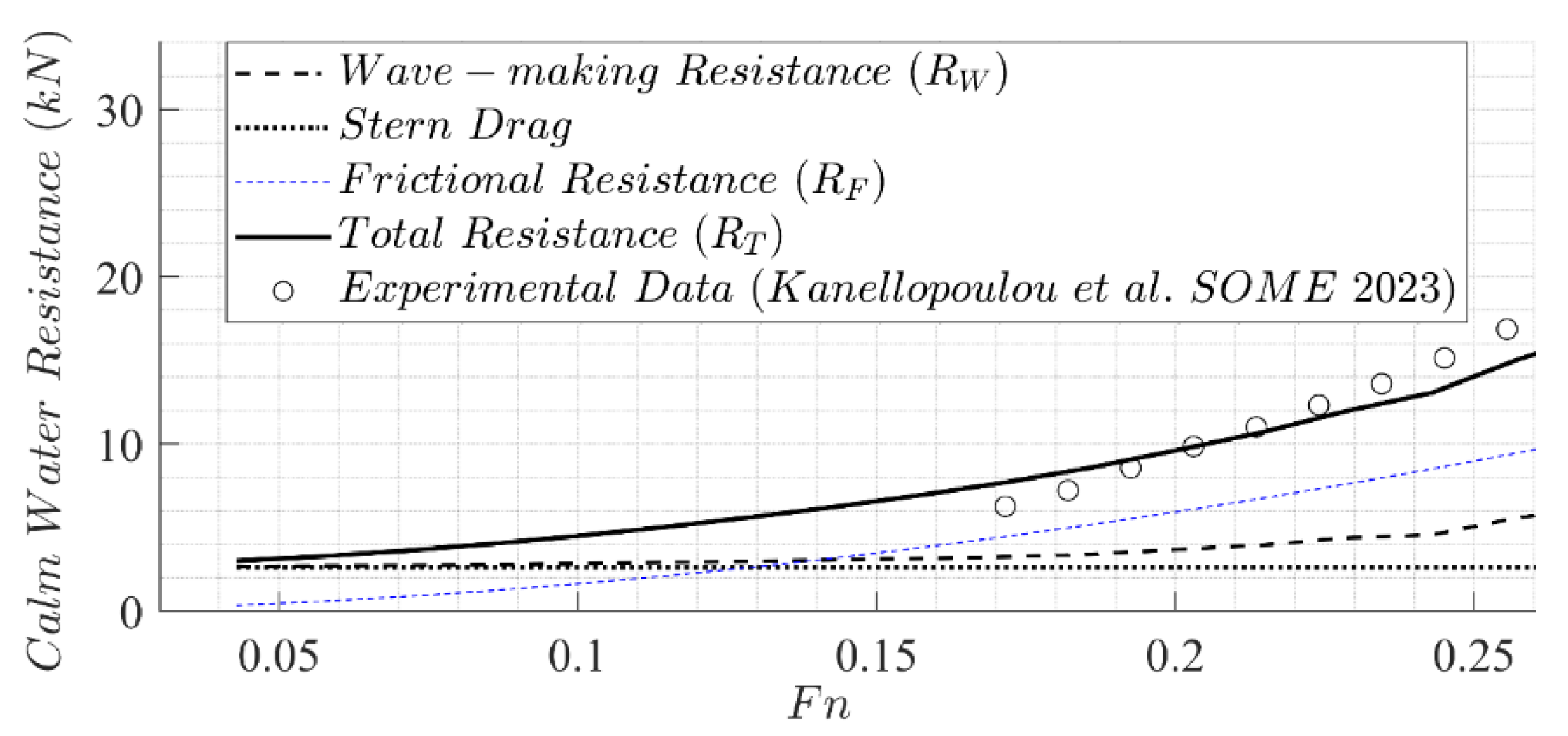
Figure 7 depicts the calm water resistance components along with the total calm water resistance, as evaluated by the present BEM scheme, and the results are compared against experimental data. As it can be observed in Figure 7, the wave-making resistance is augmented by a stern drag term resulting from the absence of hydrostatic pressure at the aft end, leading to an overestimation of the total resistance at low Froude numbers, as expected from the present scheme. In the context of linearized theory, this drag remains unchanged at different speeds. Apart from that, the results demonstrate good agreement with the experimental data within the range of Froude number . For higher values, the present model underestimates the resistance. However, significantly better agreement with the experimental data can be obtained by considering the nonlinear problem, including dynamic trim effects. These findings will be further explored in future extensions of the present work.

Figure 7.
Calm water resistance components and comparison with experimental data [9].
2.3. Formulation of the Unsteady Problem
The dynamic motions of the vessel, based on the prevailing sea conditions, are derived using standard linear hydrodynamic analysis in the frequency domain. In particular, assuming that all time-dependent quantities oscillate harmonically in the form ), where denotes the encounter frequency in and , the problem is transferred to the frequency domain using the following representation for the total unsteady potential function,
In Equation (26), denotes the incident wave height, is the gravitational acceleration, is the complex amplitude of the vessel’s response towards the -th generalized direction, is the angle of incidence of the wave field with respect to the -axis and is the vessel’s velocity in the -direction. The encounter frequency is defined as
where is the absolute frequency of the incident field (as observed from a nonmoving reference frame) and is the wavenumber, considering propagation in deep water. Finally, is the total complex unsteady potential, which comprises all the unsteady subfields and is defined as
In Equation (28), and , respectively, stand for complex amplitudes of the incident and the diffracted subfields. Furthermore, is the complex potential of the radiation field generated by a unit amplitude oscillation of the vessel along the generalized direction.
The incident potential function is considered known and equal to
The unsteady field is computed by modeling the whole domain, since it does not present symmetries, except in the special cases where equals or degrees. Furthermore, the transom sterns of both demi-hulls are modeled as vertical boundaries, incorporated in , omitting the false body representation discussed in the previous section. The diffraction and the six radiated fields are obtained as solutions to the following BVPs:
In Equation (33), denotes the components of the generalized normal vector, defined as. Consequently, the vessel’s DoF is defined as translational motion along the axis for or rotational motion around the axis for . The quantities , appearing in Equation (33) are defined as functions of the derivatives of the relative flow velocity of the steady field at the mean position of the wetted surface. The latter quantities mainly involve higher-order derivatives of the perturbation potential due to the motion of the ship at a constant speed (see e.g., ref. [18]), and after linearization, they can be approximated by
Numerical solutions to the above BVPs are obtained using a low-order BEM, which employs piecewise constant source distributions on quadrilateral boundary elements. The seven unknown fields are represented by the following integral:
The above BVPs are treated by a low-order panel method based on simple singularity (source) distribution on quadrilateral elements. The radiating behavior of the diffraction, as well as the six radiation subfields at infinity, is treated by adopting a Perfectly Matched Layer (PML) technique. This technique is utilized to attenuate the evaluated solutions far from the vessel’s position and prevent the occurrence of numerical reflections from the outer layers of the computational mesh. The PML is implemented by complexifying the frequency parameter , involved in the Free Surface BC [Equation (31)], using an appropriately defined imaginary component. The parameter is redefined as
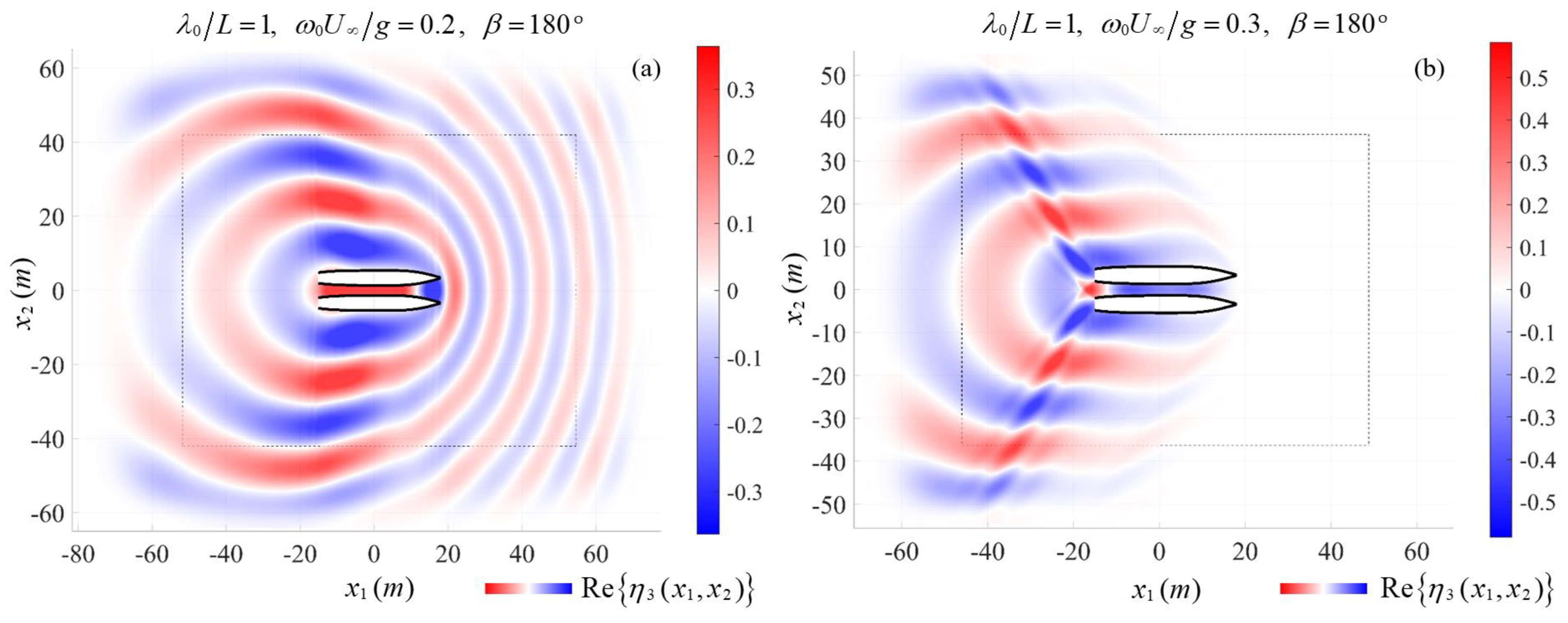
In Equation (37), stands for the wavelength that propagates at frequency and is not affected by the background flow. This corresponds to the wavelength of the diffraction and radiation fields along the -direction. Conversely, the wavelengths of the field components propagating along the -direction are significantly affected by the background flow. Specifically, the wavelengths aft of the stern are elongated, while compressed wavelengths are generated ahead of the bow in the subcritical case (for head seas). In supercritical cases, the diffraction and radiation subfields do not include components propagating toward the positive -axis. This can be clearly observed in Figure 8, which illustrates the real part of the free surface elevation generated by the unit amplitude heaving oscillation of the vessel for a fixed absolute frequency corresponding to , at two different speeds, respectively falling into the subcritical (a) and supercritical (b) regimes. Optimal values for the parameters c and n, involved in Equation (37), are selected for minimizing the numerical reflections; see [19]. The PML activation curves are also depicted in Figure 8 using dashed lines. The evaluation of the acceleration in the -direction, which is involved in Equation (31), is achieved by using the discrete Dawson operator, described in the previous section. This suggests that the boundary mesh used for evaluating the involved unsteady subfields also comprises streamline-like lines on the free surface resulting in a rectangular mesh geometry.

Figure 8.
Real part of the free surface elevation induced by unit amplitude oscillation of the vessel in heave. (a) —subcritical; (b) —supercritical. The dashed lines represent PML activation curves.
After obtaining all the subfields, the response vector of the vessel in 6 DoF is evaluated as the solution to the following system of equations:
In Equation (38), the inherent inertia of the vessel is modeled via the tensor , which equals
where the diagonal matrix models the inertia of the translational degrees of freedom with respect to the applied forces and is defined as
with denoting the vessel’s mass and the submerged volume (of both demihulls). The diagonal elements of the matrix , which models the inertia of the rotational degrees of freedom with respect to the applied moments, equal the corresponding moments of inertia of the vessel with respect to the selected coordinate system and are evaluated as
where represents the radius of gyration about the axis. In the following, the radii of gyration are defined as, and the products of inertia and are assumed to be zero due to symmetry relative to the longitudinal axis. Additionally, due to lack of detailed information and assuming symmetry of the mass distribution relative to the beam axis —even without explicit symmetry in the geometry—the product is also considered negligible, making the matrix also diagonal. The submatrices and are defined as follows:
where is the position vector of the center of gravity with respect to the origin, which is taken to be the center of flotation. The longitudinal position of is taken to coincide with that of the center of buoyancy, which is evaluated as the center of the submerged volume, to ensure that the vessel maintains an even keel. The vertical position of the center of gravity is placed at one-third of the hull depth measured from the keel, since this positioning represents a common approximation in ship design that supports accurate stability.
The added inertia of the vessel is represented by the matrix , where the elements correspond to the components of the radiation loads, induced by the field on the DoF, in phase with the acceleration. The elements of the hydrodynamic damping matrix are determined by the components that are in phase with the velocity. The above radiation forces and moments are computed by integrating the pressure exerted by the radiation field on , multiplied by the component of the normal vector corresponding to the DoF. Therefore, the hydrodynamic coefficients (added mass and hydrodynamic damping) are computed using the following equation
It is noted that the above matrices are dependent on the encounter frequency, and therefore, they also depend on the direction of propagation of the incident field, apart from the absolute frequency and the speed at which the vessel moves. The hydrostatic restoring forces are modeled via Matrix . As concerns the transitional DoFs, only vertical movements induce hydrostatic restoration and thus . Regarding the rotational DoFs, since the origin has been selected to coincide with the center of floatation (centroid of the water plane), all the first-order moments as well as the products of inertia of the waterplane are zero. Based on the above observations, the nonzero elements of are the following:
where denotes the waterplane, is the waterplane surface, is the vertical distance between the center of buoyancy and the center of gravity and is the metacentric height of the vessel with respect to the axis. The additional matrix , defined as,
represents additional damping and coupling effects on the dynamic behavior of the vessel due to forward motion. In the context of linear theory, the effect of arises since products of the form are comparable to linear terms in the equations of motion and thus cannot be neglected after linearization; see [18,20,21].
Finally, the forces and moments acting on the hull are evaluated by integration of the pressure induced by the incident and the diffracted subfields on the wetted surface. In particular, the components of the Froude–Krylov and diffraction forces are computed, taking into account the vessel’s forward motion by the following equation [20,21]:
2.4. Estimation of Added Wave Resistance
The steady-flow effects concerning the numerical computation of the added wave resistance have been discussed by several authors; see, e.g., the work by Lee and Kim [22] and the references cited therein. In the case of the present linearized model formulated in the frequency domain, various time-harmonic components result in zero or negligible contributions to the mean value of added wave resistance. For the present analysis’ purpose, the mean added wave resistance of the steady traveling vessel is estimated by the following two terms:
In Equation (51), denotes the vertical hull slope angle at the mean draft. In the above equations, the added resistance components are evaluated as mean values of the corresponding squared time-dependent quantities over one encounter period, justifying that both right-hand sides of Equations (50) and (51) include a term of that was factored out as the mean value of . The integral of Equation (50) is defined over the mean wetted surface, while the integral of Equation (51) is evaluated over the calm waterline. Moreover, in the latter equation, stands for the free surface elevation corresponding to the unsteady problem,
where is the total complex potential, which includes all eight subfields involved in Equation (28), with the six radiated subfields scaled by the complex amplitude of the vessel’s response in the corresponding DoF, as computed by Equation (38).
2.5. Model Verification
In this section, results from the present unsteady BEM model are compared against experimental data for verification purposes. The data are based on experiments in head waves conducted in 2023 in the towing tank of the Laboratory of Ship and Marine Hydrodynamics (LSMH) of the National Technical University of Athens (NTUA), in the framework of the ECLAT research project; see also [9]. The tests were conducted on a 1:10 scale, and the experimental data are reported in the NTUA Technical Report No: NAL-353-F-2023. Figure 9a,b presents the present model predictions for the twin-hull RAOs in heave and pitch along with the corresponding experimental values. Both the numerical and experimental data refer to (corresponding to for the prototype) and head seas with waveheight and absolute frequency corresponding to wavelength equal to . Additionally, Figure 9c illustrates the calculated added wave resistance for various incident wave frequencies where it is compared with experimental measurements at specific frequencies shown by using symbols. The latter are obtained as the difference in the total resistance in harmonic waves and the calm-water resistance of the twin hull in the same draft and forward speed. The present BEM results show quite good agreement with the experimental data, indicating the model’s reliability as concerns the prediction of the vessel’s dynamic behavior, as well as the added resistance. The minor differences observed are due to higher-order nonlinear effects that are not modeled by the discussed method.
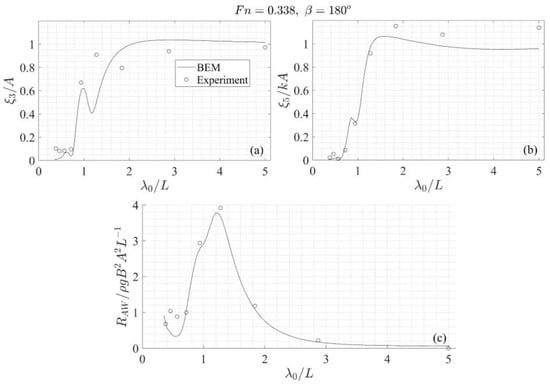
Figure 9.
Numerical results obtained by the unsteady BEM scheme concerning responses in harmonic head seas and comparison with experimental data for the twin-hull vessel at . (a) Heave RAO, (b) Pitch RAO and (c) RAO of Added Resistance.
3. Case Study
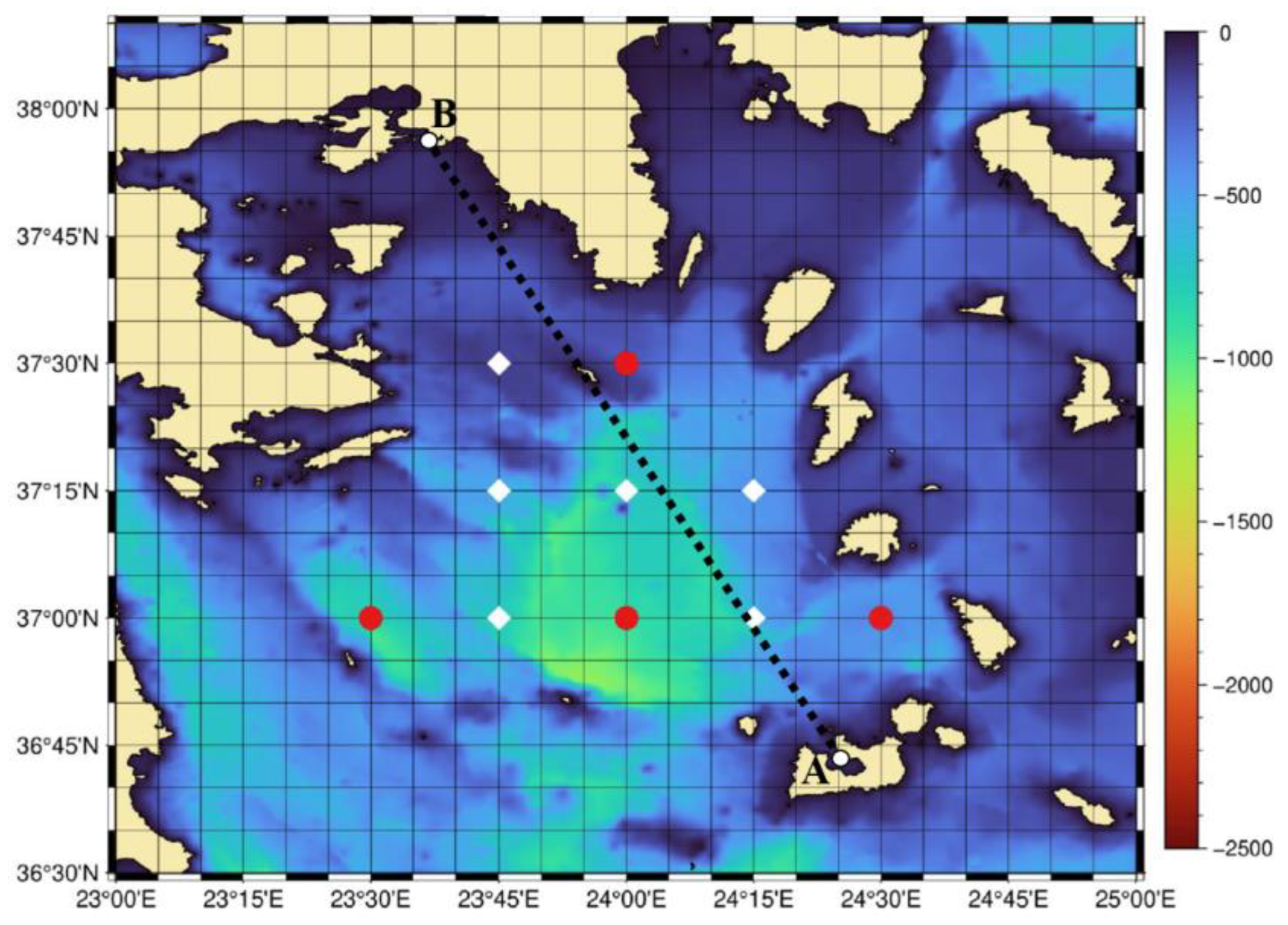
As an indicative scenario, the twin-hull vessel is considered to be operating in the Saronic Gulf, Central Aegean Region, concerning a line that connects Milos Island with Piraeus port, as shown by the track AB in Figure 10. The route’s total distance is 82 NM. The selected operating speed corresponds to and the total travel duration is approximately . For the scope of this case study and in order to provide quantified results, the vessel is considered to depart at 6:00 and navigate along the route illustrated in Figure 10 with a bearing of 332.65°, heading northwest. The reverse route is followed during nighttime, and the trip is repeated on a daily basis. The arrangement of panels on the upper deck, consisting of 123 panels with an area of each, is shown in Figure 11. A zero-tilt configuration is employed, although it is not the optimal selection to maximize energy absorption in the considered latitude, to avoid issues concerning increased wind resistance as well as space utilization. In particular, the influence of wind resistance, which is typically proportional to the area normal to the airflow direction, is assumed to be negligible and has been omitted in the context of the present study. The selection of zero-tilt panels suggests that any arbitrary selection of azimuth angle would be equivalent as concerns the energy yield of the installed system. However, since dynamic responses are expected to provoke instantaneous changes to the tilt angle, the azimuth angle is set to 62.65° (normal to the vessel’s direction). The calm water resistance is used as evaluated from the steady BEM model discussed earlier. For simplicity, the draft of the vessel is retained unchanged as compared with the previous sections. Considering that the studied vessel’s TPC is approximately 2.46 tons/cm at , the addition of the solar panels is not expected to significantly alter the draft, with an anticipated increase of about , assuming the panels weigh approximately 10 kg/m2. Furthermore, as illustrated in Figure 11, the arrangement of the panels ensures that the weight is distributed evenly across the vessel, thus minimizing any potential impact on the weight distribution.

Figure 10.
Indicative route (dotted line) from Milos Island—point A (36°43′ N, 24°25′ E)—to Piraeus port—point B (37°56′ N, 23°38′ E)—with a total distance of 82 NM.
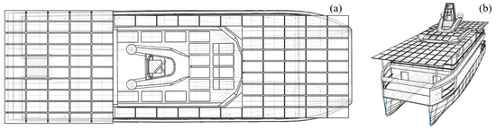
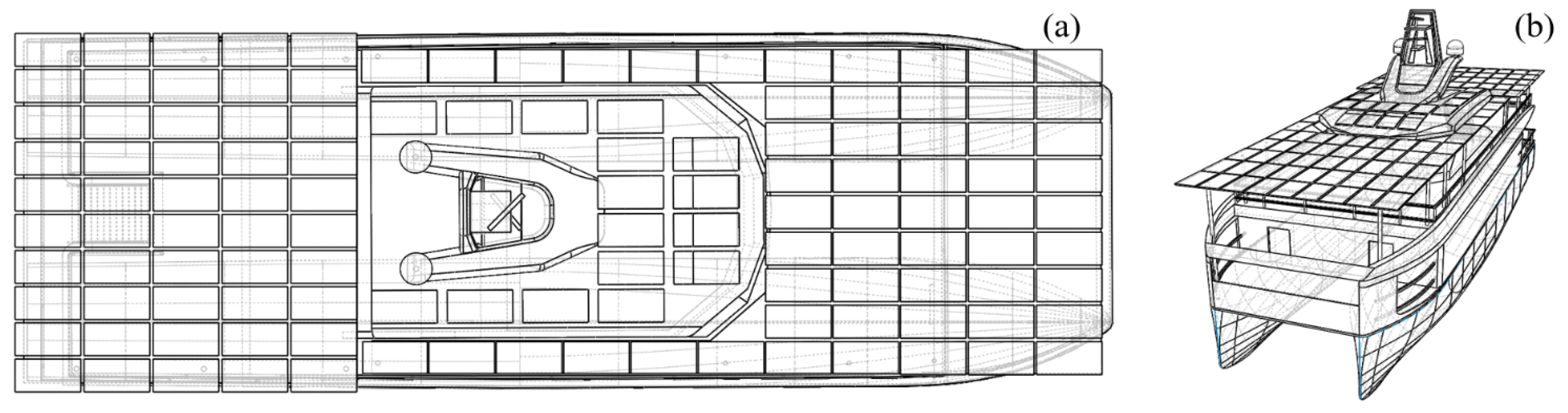
Figure 11.
(a) Top view and (b) 3D view of the considered arrangement of 123 solar panels on the twin-hull vessel.
The mean added wave resistance, as well as the spectra of dynamic responses, is computed by the unsteady BEM model in conjunction with climatological data of the considered region acquired from the Copernicus database [https://www.copernicus.eu/en/access-data (accessed on 20 July 2024)].
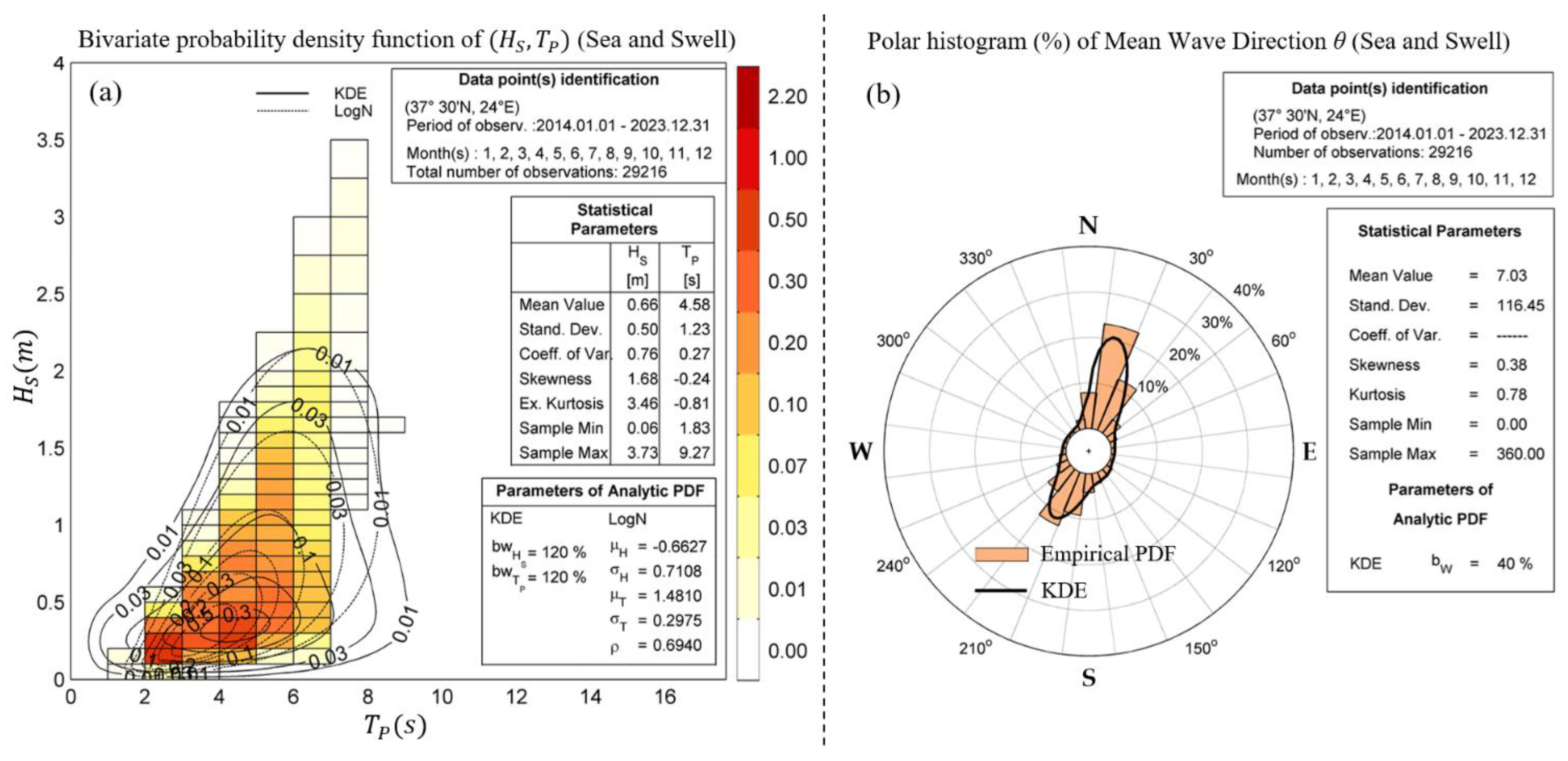
In particular, the wave climatology of the point (37°30′ N, 24° E) is selected as representative of the considered route. The bivariate probability density function of significant wave height and peak period is depicted in Figure 12a, along with a polar histogram of mean wave direction (Figure 12b). Based on the above climatological data of the Saronic Gulf and Central Aegean Sea area, the prevailing wave directions relative to ship track correspond to (i) head quartering seas and (ii) following quartering seas . In order to illustrate the applicability of the present model, the mean values of the distribution corresponding to peak wave period equal and significant wave height are considered in conjunction with head-quartering seas In this case, the corresponding peak encounter frequency is and the parameter equals , indicating supercritical conditions at peak frequency.
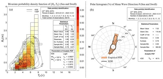
Figure 12.
Wave climatology based on data of point (37°30′ N, 24° E) from Copernicus database. (a) Bivariate probability density function of and (b) polar histogram (%) of mean wave direction ().
All angular responses are expected to contribute to the dynamics of the installed solar system. However, given that rolling motion is expected to have the most significant impact, in the context of the present case study, the tilt angle of the PV configuration is substituted by the corresponding dynamic value, which is approximated by summing the static tilt angle with the instantaneous roll response of the vessel, as described in more detail in the sequel.
Moreover, the vessel is considered to travel during daylight hours, exploiting solar power for the partial coverage of the power needs and return during nighttime. More realistic scenarios, based on long-term time series of wave conditions modeled by considering varying sea states and relative wave directions, including beam and following seas along the route, as well as contributions of all angular responses, will be developed and applied in future extensions of the present work, supporting a full technoeconomic analysis of solar-power-augmented vessels.
3.1. Selected Results of Wave Responses and Added Wave Resistance
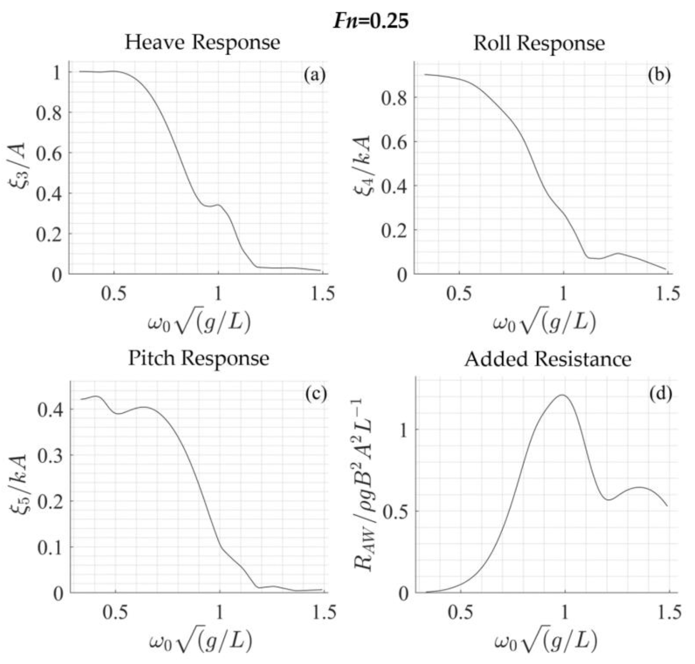
For the considered case, corresponding to and , selected results are presented in Figure 13, as obtained by the unsteady BEM model, discussed in Section 2. The results include the vessel’s response in heave, roll, and pitch motions, as well as the computed normalized added resistance. The curves depicted in Figure 13 demonstrate that the limiting behavior at low frequencies is in line with theoretical expectations. In particular, the heave response amplitude tends to unity, while the roll and pitch response amplitudes converge to and , respectively, confirming that the discussed model properly modulates the angular responses with respect to the angle of incidence.

Figure 13.
Calculated results for head quartering seas : Response Amplitude Operators (RAOs) of (a) heave, (b) roll, and (c) pitch motions, as well as (d) RAO of added resistance. .
The wave spectrum concerning the sea state characterized by peak period and significant wave height is modeled using a Bretschneider spectrum,
Subsequently, the spectrum is redefined in terms of the encounter frequency , while maintaining the energy distribution as follows:
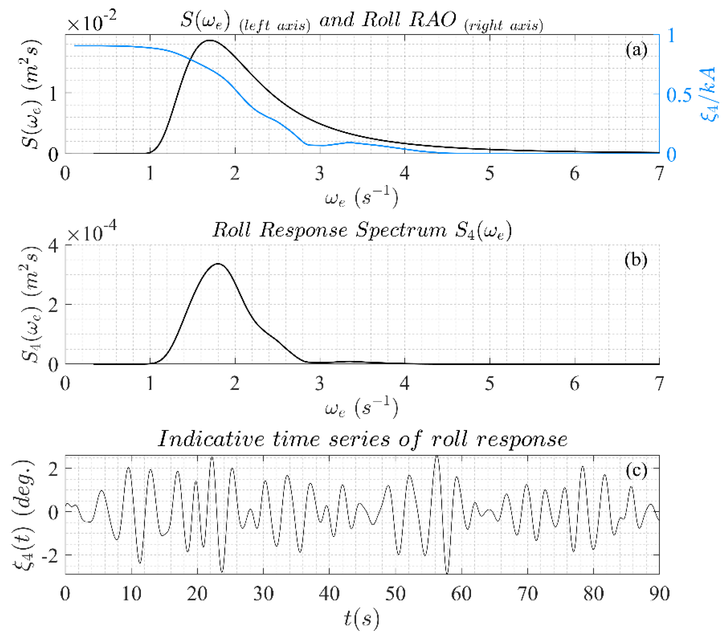
Finally, the roll response spectrum is evaluated as
The sea spectrum and the corresponding roll response spectrum in terms of the encounter frequency are depicted in Figure 14a,b. The roll RAO is plotted in Figure 14a, in terms of the encounter frequency, using a distinct vertical axis for clarity purposes. An indicative time series of rolling motion, obtained by applying the random-phase model, is presented in Figure 14c; see also [23,24]. The latter quantity is used as a disturbance of the panel tilt angle due to the wave-induced motions. The results concerning the solar power output during the daily hours of the trip over a Typical Meteorological Year (TMY) are presented and discussed in the next section.
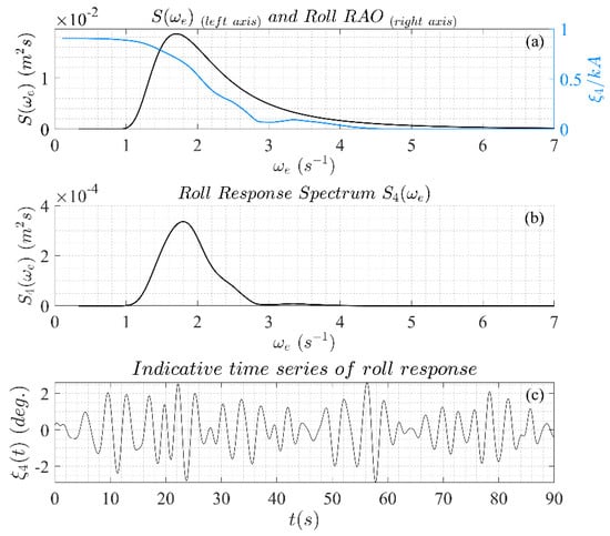
Figure 14.
(a) Sea spectrum and corresponding roll RAO and (b) response spectrum in terms of the encounter frequency. (c) Indicative time series of rolling motion.
3.2. Estimation of Energy Needs and PV Contribution
The vessel can cover a distance of 40 nautical miles at a speed of 13 kn. At the latter speed, the calm water resistance equals 49.5 kN, based on experimental measurements [9]. Moreover, the auxiliary loads (lighting, air-conditioning, equipment, etc.) for the studied vessel are estimated to be [25]. Considering a Depth of Discharge (DoD) of 80% for the battery and given its capacity (see Table 1), it is concluded that the propulsion system has a total efficiency of . For the considered speed, corresponding to , the calm water resistance is (see Figure 7). The added resistance is imported in the analysis using the value of its response spectrum, based on the considered sea state, expressed in terms of the encounter frequency. The latter parameter contributes to the total resistance by . Based on the above, the total power consumption equals
The real-time contribution of the PV system is calculated based on the method presented in ref. [24]. The energy efficiency of the installed photovoltaic system is affected by several parameters such as humidity, ambient temperature, and wind speed. Moreover, certain factors encountered in the marine environment help maintain lower operating temperatures and optimize performance. In this work, in order to proceed to a preliminary calculation of the extent to which the considered system can compensate for the energy needs of the vessel, accounting for the effect of rolling motion, as well as added wave resistance in the specific sea state, the following equation is used to evaluate the power delivered by the solar system:
In Equation (57) is the generated power, which depends on the panel efficiency , the total surface area , the global irradiance , the difference between the cell temperature and the standard test temperature , and the temperature coefficient . In order to estimate energy production data, a representative value of efficiency is assumed at , which falls within the upper limit of the current range for solar cell efficiency; see, e.g., ref. [26]. The total area covered is and the installed system’s nominal power is approximately . The temperature coefficient is set to , based on estimates for silicon panel technology; see also [27]. The total radiation received by the panels comprises the direct (beam) radiation , the diffuse horizontal irradiation , and the reflected irradiance component . The direct and diffuse components are calculated as follows [28]:
where is the Direct Normal Irradiance and the Diffuse Horizontal Irradiance. For the present case study, the latitude is approximated by its value at the midpoint of the route . Moreover, is the earth’s declination and , , respectively, denote the panels’ tilt and azimuth angles. The latter parameters are set to and , as discussed earlier in the present chapter. Furthermore, is the hour angle defined in terms of the Local Solar Time, which in turn is defined based on the longitude and the equation of time (EOT). The longitude of operation is also approximated by its value at the midpoint of the route . As concerns the reflected irradiance component , it is approximated using where the coefficient , which quantifies the albedo effect, is set to for the considered marine environment.
The effect of rolling motion is introduced in the analysis, directly affecting the angle of incidence (AOI), by considering the time series of the actual instantaneous tilt angle of the panels, defined as
In Equation (63), represents simulated time series of roll response, obtained by applying the random phase model; see Figure 14c.
Data regarding Direct Normal Irradiance , Diffuse Horizontal Irradiance , and other environmental factors such as temperature, humidity, and wind speed are derived from the PVGIS SARAH2 database. The data represent a Typical Meteorological Year (TMY) with an hourly temporal resolution and are provided by PVG tools [https://re.jrc.ec.europa.eu/pvg_tools/en/ (accessed on 3 August 2024)]. The dataset includes information concerning dry-bulb temperature and relative humidity , from which the ambient temperature is evaluated following the method described in ref. [29],
In Equation (64), is the apparent temperature, is the wind speed, and denotes the vapor pressure in , evaluated as
where is the dew point temperature which is estimated based on the relative humidity , using the approximate formula that is valid for After calculating the ambient temperature, the panel cell temperature is estimated using the following correlation provided by Sandia National Laboratories:
where is the incident solar irradiance on the panels and are parameters dependent on the module construction, which for glass/cell/polymer sheet panels are defined as [see https://pvpmc.sandia.gov/modeling-steps/2-dc-module-iv/module-temperature/sandia-module-temperature-model/ (accessed on 3 August 2024)].
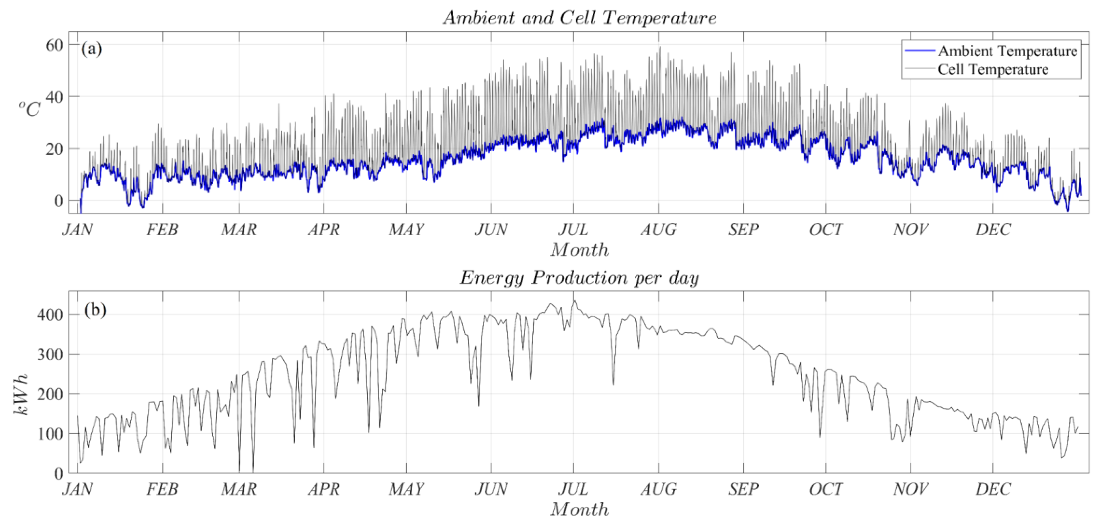
Numerical results concerning the ambient and cell temperatures as well as the daily energy production of the considered system are illustrated in Figure 15. It is worth noting that electrical system losses are not accounted for in the present study but will be included in future extensions, along with the impact of all angular responses, as well as varying sea states and relative wave direction.
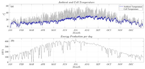
Figure 15.
(a) Ambient temperature and cell temperature of the installed solar system and (b) daily energy production in kWh during a TMY.
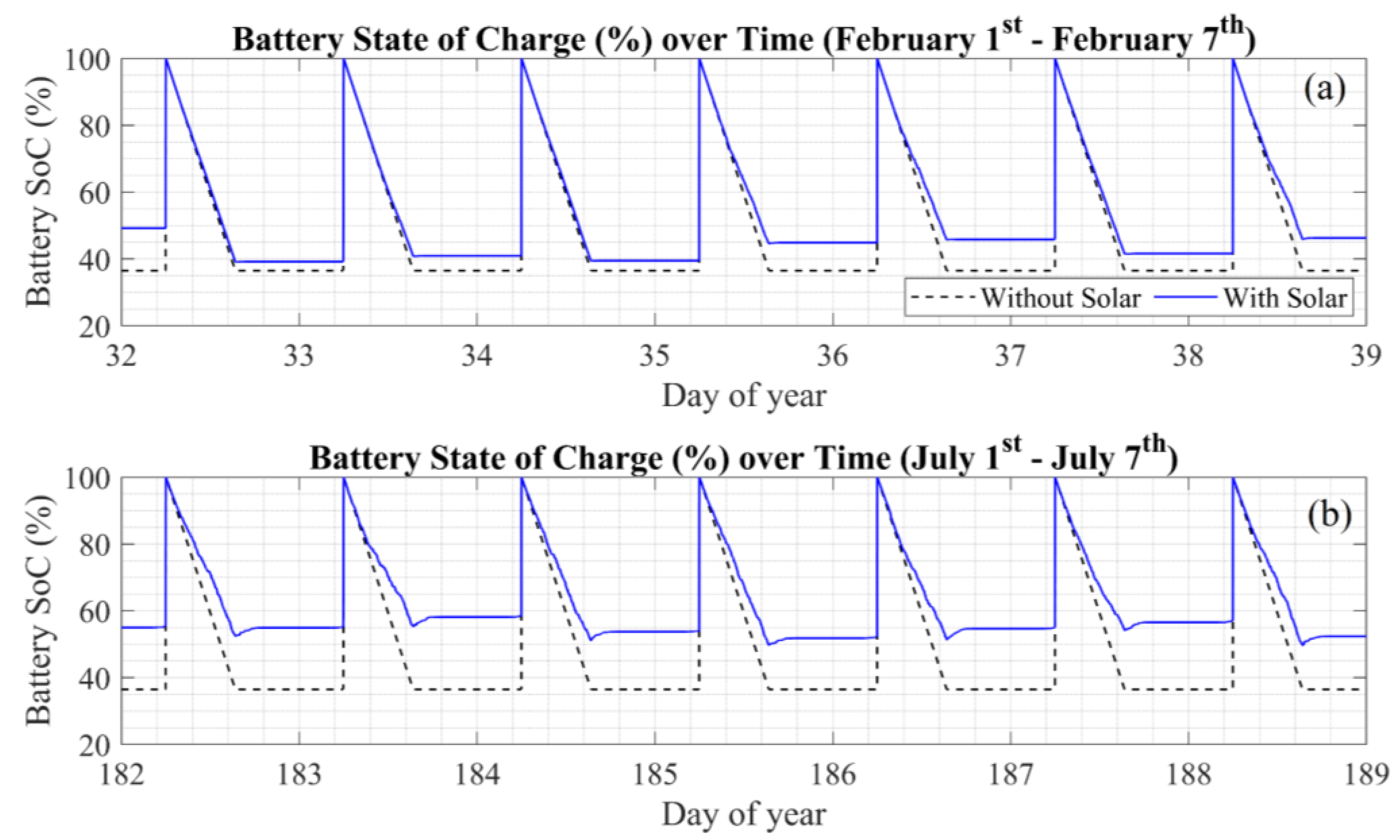
Figure 16 illustrates the State of Charge (SoC) of the vessel’s battery, as it evolves with and without the auxiliary solar system, for two indicative weeks of the year, corresponding to winter and summer conditions, respectively.

Figure 16.
State of Charge (SoC) of battery, as it evolves with and without the auxiliary solar system, for two indicative weeks of the year, corresponding to (a) winter and (b) summer conditions.
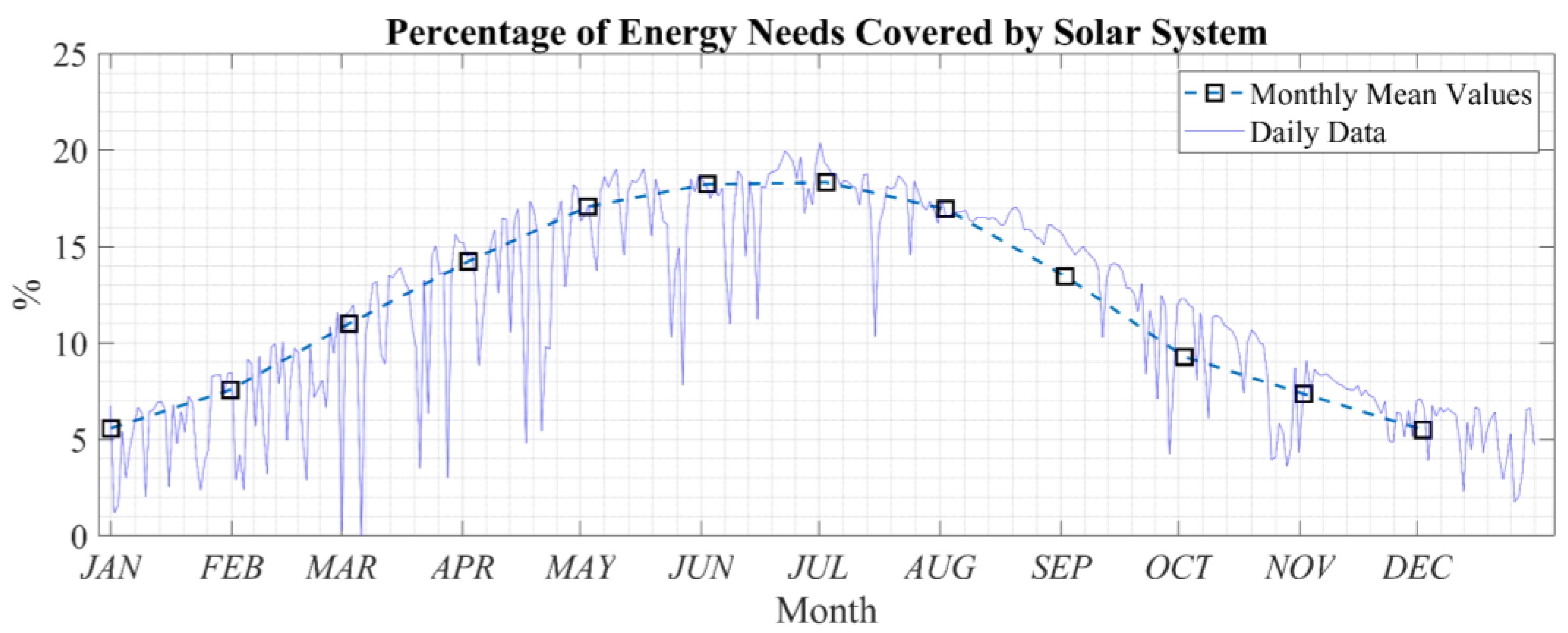
Charging from external sources is assumed to restore the battery to fully charged before each departure. For the scope of the present case study, the charging is considered instantaneous to simplify the calculations. Figure 17 depicts the percentage of energy needs covered by the auxiliary solar system on a daily basis and in average monthly values. This percentage ranges from approximately 5% in winter months to a maximum of 18.3% during summer. The mean percentage of power needs covered within a TMY equals 13.6%.
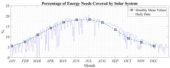
Figure 17.
Percentage of energy needs covered by the auxiliary solar system on a daily basis and in average monthly values.
4. Conclusions and Discussion
In this work, a novel Boundary Element Method (BEM) formulation is presented for predicting the resistance, as well as the hydrodynamic behavior, of twin-hull vessels traveling at low speeds, aiming to quantify the benefits of integrating auxiliary solar systems onboard. The analysis is based on a case study concerning a 33 m long electric twin-hull vessel. The placement of solar panels on deck is discussed and their utilization in terms of real-time energy generation is assessed, aiming to partially cover the energy needs, while also reducing carbon emissions. Numerical results are presented, verified, and discussed regarding calm water resistance and added resistance, as well as the wave-induced motions of the vessel. Moreover, the energy generated by the integrated solar system is quantified and combined with power demand estimates to assess the percentage of power needs covered without relying on external sources. Various operational factors are considered in predicting the power needs as well as the power production by the auxiliary solar system. Based on the selected parameters and operation conditions, the results indicate that the considered system contributes by 13.6% on average to the coverage of the total power requirements, with the latter percentage ranging from 5% to around 18.3% throughout a TMY. The direct effect of dynamics on the solar system’s energy yield is limited to rolling motion, while the coupled effects by all angular DoFs will be examined in future extensions of the present work. Future works will also be directed toward the investigation of the panels’ vulnerability to environmental parameters, including potential damages from strong winds or severe storms, as well as salt deposition, which can affect their efficiency and longevity.
Other interesting extensions include the investigation of installing additional renewable energy sources on ships, such as flapping-foil thrusters placed at the bow. The latter technology has been numerically and experimentally studied in ref. [30], and the results suggest that it offers increased dynamic stability and a reduction in added wave resistance while also exploiting energy from dynamic motions and directly converting it to useful propulsive power. Consequently, the cumulative advantages of multiple renewable sources could accelerate the transition towards more sustainable maritime solutions.
Author Contributions
Conceptualization, K.B.; methodology, K.B. and A.M.; software, A.M. and K.B.; validation, A.M.; writing—original draft preparation, A.M.; writing—review and editing, K.B.; visualization, A.M.; supervision, K.B. All authors have read and agreed to the published version of the manuscript.
Funding
This research received no external funding.
Institutional Review Board Statement
Not applicable.
Informed Consent Statement
Not applicable.
Data Availability Statement
The original contributions presented in the study are included in the article, further inquiries can be directed to the corresponding author.
Acknowledgments
The doctoral studies of A. Magkouris are currently supported by the Special Account for Research Funding (E.L.K.E.) of National Technical University of Athens (N.T.U.A.), operating in accordance with Law 4485/17 and National and European Community Law.
Conflicts of Interest
The authors declare no conflicts of interest.
References
- Minak, G. Solar Energy-Powered Boats: State of the Art and Perspectives. J. Mar. Sci. Eng. 2023, 11, 1519. [Google Scholar] [CrossRef]
- Leung, C.P.; Cheng, K.W.E. Zero emission solar-powered boat development. In Proceedings of the 2017 7th International Conference on Power Electronics Systems and Applications—Smart Mobility, Power Transfer & Security (PESA), Hong Kong, China, 12–14 December 2017; pp. 1–6. [Google Scholar]
- Ajlif, M.A.; Joseph, S.C.; Chacko, R.V.; Joseph, A.; Jayan, P.; Raghavan, D.P. LVDC Architecture for Energy Efficient House Boat Hotel Load System. In Proceedings of the 2019 National Power Electronics Conference (NPEC), Tiruchirappalli, India, 13–15 December 2019; pp. 1–5. [Google Scholar]
- Tercan, Ş.H.; Eid, B.; Heidenreich, M.; Kogler, K.; Akyürek, Ö. Financial and Technical Analyses of Solar Boats as A Means of Sustainable Transportation. Sustain. Prod. Consum. 2021, 25, 404–412. [Google Scholar] [CrossRef]
- Spagnolo, G.S.; Papalillo, D.; Martocchia, A.; Makary, G. Solar-Electric Boat. J. Transp. Technol. 2012, 2, 144–149. [Google Scholar] [CrossRef]
- Hasan, T.; Jamaludin, S.; Nik, W.W.; Rajib, M.H. Study and analysis of a solar electric boat with dynamic design strategy in efficient way. In Proceedings of the 13th International Conference on Marine Technology (MARTEC 2022), Dhaka, Bangladesh, 21–22 December 2022. [Google Scholar]
- Kambezidis, H.D.; Mimidis, K.; Kavadias, K.A. The Solar Energy Potential of Greece for Flat-Plate Solar Panels Mounted on Double-Axis Systems. Energies 2023, 16, 5067. [Google Scholar] [CrossRef]
- ITTC. Recommended Procedures and Guidelines, Testing and Data Analysis Resistance Test. In Proceedings of the International Towing Tank Conference, Fukuoka, Japan, 14–20 September 2008. [Google Scholar]
- Kanellopoulou, A.; Zaraphonitis, G.; Grigoropoulos, G.; Liarokapis, D. Extensive hullform optimization studies for a series of small electric catamaran ferries. In Proceedings of the 8th International Symposium on Ship Operations, Management & Economics (SOME), Athens, Greece, 7–8 March 2023. [Google Scholar]
- Noblesse, F. Alternative integral representations for the Green function of the theory of ship wave resistance. J. Eng. Math. 1981, 15, 241–265. [Google Scholar] [CrossRef]
- Wang, H.; Zhu, R.; Gu, M.; Gu, X. Numerical investigation on steady wave of high-speed ship with transom stern by potential flow and CFD methods. Ocean Eng. 2022, 247, 110714. [Google Scholar] [CrossRef]
- Couser, P.R.; Wellicome, J.F.; Molland, A.F. An Improved Method for the Theoretical Prediction of the Wave Resistance of Transom-Stern Hulls Using a Slender Body Approach. Int. Shipbuild. Prog. 1999, 45, 331–349. [Google Scholar]
- Doctors, L.J. A Numerical Study of the Resistance of Transom-Stern Monohulls. Ship Technol. Res. 2015, 54, 134–144. [Google Scholar] [CrossRef]
- Sinha, S.N.; Gupta, A.K.; Oberai, M.M. Laminar Separating Flow over Backsteps and Cavities Part I: Backsteps. AIAA J. 1981, 19, 1527–1530. [Google Scholar] [CrossRef]
- Katz, J.; Plotkin, A. Numerical (Panel) Methods. In Low-Speed Aerodynamics, 2nd ed.; Cambridge Aerospace Series; Cambridge University Press: Cambridge, UK, 2001; pp. 206–229. [Google Scholar]
- Dawson, C. A practical computer method for solving ship-wave problems. In Proceedings of the 2nd International Conference on Numerical Ship Hydrodynamics, Berkeley, CA, USA, 19–21 September 1977; pp. 30–38. [Google Scholar]
- Molland, A.F.; Turnock, S.R.; Hudson, D.A. Ship Resistance and Propulsion: Practical Estimation of Ship Propulsive Power; Cambridge University Press: Cambridge, UK, 2011; p. 544. [Google Scholar]
- Ohkusu, M. Advances in Marine Hydrodynamics; Computational Mechanics Publications: Boston, MA, USA, 1996. [Google Scholar]
- Belibassakis, K.; Bonovas, M.; Rusu, E. A Novel Method for Estimating Wave Energy Converter Performance in Variable Bathymetry Regions and Applications. Energies 2018, 11, 2092. [Google Scholar] [CrossRef]
- Lewis Edward, V. Motions in Waves. In Principles of Naval Architecture (Second Revision), Volume III—Motions in Waves and Controllability; Society of Naval Architects and Marine Engineers (SNAME): Alexandria, VA, USA, 1989. [Google Scholar]
- Lewandowski, E.M. The Dynamics of Marine Craft: Maneuvering and Seakeeping; World Scientific Publishing Co. Pte Ltd.: Singapore, 2004. [Google Scholar]
- Lee, J.H.; Kim, B.S.; Kim, Y. Study on Steady Flow Effects in Numerical Computation of Added Resistance of Ship in Waves. J. Adv. Res. Ocean Eng. 2017, 3, 193–203. [Google Scholar] [CrossRef]
- Magkouris, A.; Belibassakis, K.; Rusu, E. Hydrodynamic Analysis of Twin-Hull Structures Supporting Floating PV Systems in Offshore and Coastal Regions. Energies 2021, 14, 5979. [Google Scholar] [CrossRef]
- Magkouris, A.; Rusu, E.; Rusu, L.; Belibassakis, K. Floating Solar Systems with Application to Nearshore Sites in the Greek Sea Region. J. Mar. Sci. Eng. 2023, 11, 722. [Google Scholar] [CrossRef]
- Margaronis, P.; Kanellopoulou, A.; Silionis, N.; Liarokapis, D.; Sofras, E.; Prousalidis, J. Holistic Design of a Twin-Hull Short-Sea Shipping Vessel With Hybrid-Electric Propulsion. In Proceedings of the 2023 IEEE International Conference on Electrical Systems for Aircraft, Railway, Ship Propulsion and Road Vehicles & International Transportation Electrification Conference (ESARS-ITEC), Venice, Italy, 29–31 March 2023; pp. 1–6. [Google Scholar]
- Ma, T.; Li, Z.; Zhao, J. Photovoltaic panel integrated with phase change materials (PV-PCM): Technology overview and materials selection. Renew. Sustain. Energy Rev. 2019, 116, 109406. [Google Scholar] [CrossRef]
- Paudyal, B.R.; Imenes, A.G. Investigation of temperature coefficients of PV modules through field measured data. Sol. Energy 2021, 224, 425–439. [Google Scholar] [CrossRef]
- Honsberg, C.B.; Bowden, S.G. Photovoltaics Education Website. Available online: www.pveducation.org (accessed on 10 July 2024).
- Jacobs, S.J.; Pezza, A.B.; Barras, V.; Bye, J.; Vihma, T. An analysis of the meteorological variables leading to apparent temperature in Australia Present climate, trends, and global warming simulations. Glob. Planet. Chang. 2013, 107, 145–156. [Google Scholar] [CrossRef]
- Belibassakis, K.; Filippas, E.; Papadakis, G. Numerical and Experimental Investigation of the Performance of Dynamic Wing for Augmenting Ship Propulsion in Head and Quartering Seas. J. Mar. Sci. Eng. 2022, 10, 24. [Google Scholar] [CrossRef]


Disclaimer/Publisher’s Note: The statements, opinions and data contained in all publications are solely those of the individual author(s) and contributor(s) and not of MDPI and/or the editor(s). MDPI and/or the editor(s) disclaim responsibility for any injury to people or property resulting from any ideas, methods, instructions or products referred to in the content. |
© 2024 by the authors. Licensee MDPI, Basel, Switzerland. This article is an open access article distributed under the terms and conditions of the Creative Commons Attribution (CC BY) license (https://creativecommons.org/licenses/by/4.0/).