Article

Development of a Hierarchical Clustering Method for Anomaly Identification and Labelling of Marine Machinery Data

by
Christian Velasco-Gallego
1,*,
Iraklis Lazakis
2 and
Nieves Cubo-Mateo
1
1
Grupo de Investigación ARIES, Universidad Nebrija, C. de Sta. Cruz de Marcenado, 27, 28015 Madrid, Spain
2
Department of Naval Architecture, Ocean and Marine Engineering, University of Strathclyde, 100 Montrose Street, Glasgow G4 0LZ, UK
*
Author to whom correspondence should be addressed.
J. Mar. Sci. Eng. 2024, 12(10), 1792; https://doi.org/10.3390/jmse12101792
Submission received: 4 September 2024 / Revised: 3 October 2024 / Accepted: 5 October 2024 / Published: 9 October 2024
(This article belongs to the Special Issue Applications of Artificial Intelligence in Marine Machinery)

Abstract

:
The application of artificial intelligence models for the fault diagnosis of marine machinery increased expeditiously within the shipping industry. This relates to the effectiveness of artificial intelligence in capturing fault patterns in marine systems that are becoming more complex and where the application of traditional methods is becoming unfeasible. However, despite these advances, the lack of fault labelling data is still a major concern due to confidentiality issues, and lack of appropriate data, for instance. In this study, a method based on histogram similarity and hierarchical clustering is proposed as an attempt to label the distinct anomalies and faults that occur in the dataset so that supervised learning can then be implemented. To validate the proposed methodology, a case study on a main engine of a tanker vessel is considered. The results indicate that the method can be a preliminary option to classify and label distinct types of faults and anomalies that may appear in the dataset, as the model achieved an accuracy of approximately 95% for the case study presented.

1. Introduction

Industrial processes are growing in scale, and thus safety is becoming a crucial matter, which is leading to an increase in safety monitoring demands [1]. To guarantee production safety and minimise risks, stable operations of industrial processes are of paramount importance ([2,3]). It is unsurprising, therefore, that the development of novel fault diagnosis frameworks increased in the fields of process safety and risk assessment [4]. Fault diagnosis can be defined as a process aimed at tracing a fault by means of its symptoms [5]. Thus, fault diagnosis is one of the most important methods to ensure safety when employing complex systems ([6,7,8]). It is a process that is widely studied and analysed by academics in sectors such as chemical ([9,10]), manufacturing ([11,12,13,14,15,16]), and transportation ([17,18,19]).
If the shipping industry is analysed in detail, the safety and reliability of marine machinery systems and components are some of the utmost challenges to be addressed [20]. The increase in complexity of marine machinery and the lack of effectiveness of traditional methods for these systems enabled the implementation of more sophisticated approaches [21]. Additionally, the limitations of conventional methods in this domain, such as the time required for diagnosticians to analyse the amount of data acquired from sensors coupled to machinery, drove the demand for developing automatic decision-making tools to assess the current health status of the monitored systems [22]. These are probably the main reasons that facilitated the employment of intelligent fault diagnosis in tandem with artificial intelligence. Accordingly, artificial intelligence is widely employed to enhance current practices regarding the fault diagnosis of marine machinery [23,24] and to enable intelligent shipping technology ([25,26]).
The application of artificial intelligence for fault diagnosis demonstrated multiple benefits and opportunities that this technology can offer. Examples include the following: (1) reduction in human error, (2) increase in the level of information and the utilisation of sensor data, (3) enhancements in communication technologies, and (4) enhancements in data analysis practices. Specifically, there was an increase in the consideration of deep learning models for fault diagnosis [27,28]. However, deep learning-based fault diagnosis methods require vast amounts of labelled data for adequate training [29]. Consequently, most of the fault diagnosis studies within the shipping sector focus mainly on the fault detection task, as the lack of fault data is still a major limitation for the implementation of artificial intelligence for fault diagnosis [30]. Furthermore, even though fault data are available, these data are usually unlabelled and/or imbalanced [31].
Hence, even though several methodologies were already proposed, there are still certain issues that need to be tackled. In this study, the lack of fault label data issue is addressed. The lack of fault data can limit most of the studies that consider deep learning approaches, as they require vast amounts of data. Additionally, even if fault data are available, these data are usually not labelled. Therefore, fault diagnosis models cannot be employed. Despite this fact, most of the analysed methodologies assume that fault label data are available, which is rare in real-world scenarios. Furthermore, after analysing all the identified papers on fault diagnosis of marine diesel engines ([32,33,34,35,36,37,38,39,40,41,42,43,44]), there is no evidence to the best of the authors’ knowledge that a methodology for the labelling of fault data was proposed. For this reason, this study aims to present a new method for the labelling of fault data. This method seeks to combine histogram similarity with hierarchical clustering analysis. Special attention is also given to the selection of the parameters that are critical for the performance of the model, such as the number of bins in the histogram and the number of clusters. Additionally, as hierarchical clustering analysis is introduced, the challenges of fault imbalance are also analysed.
The paper is structured as follows: Section 2 presents the existing related work and state-of-the-art on this topic. Section 3 describes the proposed methodology. Section 4 introduces and discusses the results obtained after the implementation of a case study on a main engine of a tanker vessel. Finally, Section 5 outlines the main conclusions and future work.

2. Literature Review

Various models were developed for the fault diagnosis of marine machinery. Specifically, the study of deep learning approaches recently saw a significant increase. For instance, a fault diagnostic approach based on an improved temporal convolutional network and generative adversarial network for data augmentation was proposed by [45]. To validate the proposed methodology, a case study on underwater thrusters was performed. The results indicate that the proposed methodology could increase the average F1-score up to 8.5% compared to the original temporal convolutional network classifier.
Analogously, a probabilistic similarity and linear similarity-based graph convolutional neural network for ship ballast water system condition monitoring was introduced by [46]. Initially, the introduced model transforms the dataset, which is related to the ship’s ballast water system, into two distinct graph structures. The first graph represents a probabilistic topology graph, while the second graph represents a correlation topology graph. This graph configuration enabled the implementation of T-SNE for probabilistic similarity and Pearson’s correlation coefficient for linear similarity. Thus, inter-sample neighbor relationships could be established. Once these relationships were determined, early fusion of the two graph structures was conducted to extract multi-scale feature information. Finally, a graph convolutional neural network was introduced. The proposed model achieved an accuracy of 97.49% on a simulated ship fault dataset case study. A multi-head attention neural network was proposed by [47], which comprised a multi-head attention mechanism, convolutional layers, and residual structure.
Additionally, a rank-order similarity of the multi-head graph attention neural network was applied by [48]. Analogous to [46], T-SNE and Spearman’s correlation coefficient were introduced to determine both probabilistic similarity and rank order similarity so that a neighbour relationship between samples could be established. Subsequently, early fusion of the two graph structures was conducted, and then a graph attention neural network, which incorporated multi-head attention, was employed. This proposed model led to an accuracy of 97.58% for the case study introduced regarding a simulated ship engine dataset. A multi-channel multi-scale convolutional neural network for ship pipeline valve leak monitoring was developed by [49]. The proposed model facilitated fault feature extraction from grayscale images and feature-level fusion application for fault classification. Thus, the impact of data redundancy and noise could be mitigated.
A balanced adaptation domain-weighted adversarial network was considered by [50]. To validate the proposed methodology, two experimental scenarios were proposed, which considered a Wärstilä9L34DF dual-fuel engine as an experimental subject, where the model achieved an accuracy of over 90% diagnostic accuracy in scenarios with complete target working condition labels.
If the application of data-driven methodologies for the fault diagnosis of marine diesel engines is analysed in detail, an additional 94 papers were retrieved utilising the following keywords in the Scopus database: “fault diagnosis”, “ship*”, and “diesel engin*”. Of all the resulting papers, the most recent ones were analysed, focusing on the period from 2020 to 2024. In total, thirteen papers were identified to fall within the area of the application of artificial intelligence for the fault diagnosis of diesel engines in the shipping industry ([36,37,38,39,40,41,42,43,44,45,46,47,48]). All of the studies considered simulated fault data generated from either simulator software or experimental setups. The fault data were then utilised to train a fault classification model. All the analysed studies employed supervised learning, which means that fault data were required for the adequate training of the implemented models. Therefore, fault labels are indispensable for the implementation of these models, even though in most real-world scenarios, the lack of fault labelling data remains a major concern due to confidentiality issues and lack of appropriate data. Consequently, the application of all the identified models may be unfeasible if fault labels are not provided in advance. For this reason, the development of methodologies, such as the one presented in this study, is of preeminent importance to ensure adequate fault label data availability. Upon further analysis of these models, it can be perceived that 54% relate the application of deep learning methodologies. Specifically, the following models were considered: convolutional neural network, back propagation neural network, adversarial neural network, long short-term memory neural network, and convolutional autoencoder. All of these models were implemented within the last two years, indicating that deep learning is gaining attention in this field. However, hyperparameter optimisation remains unexplored, as there is no evidence that the analysed studies incorporating deep learning considered hyperparameter optimisation algorithms. Nonetheless, deep learning still demonstrated its capability to accurately perform fault diagnosis tasks.
Despite the undeniable benefits of deep learning methodologies for fault diagnosis of marine machinery, their limitations and disadvantages cannot be diminished. For instance, deep learning methodologies usually require vast amounts of data to perform effectively. Nevertheless, the amount of fault data available in this sector is usually limited. For this reason, either unsupervised or semi-supervised models are employed when fault data are not available. For instance, a semi-supervised principal component analysis was applied to diesel engine fault diagnosis by [32]. Multi-parameter prediction models are also usually employed for early detection of faults. An example of this is [33], which introduced a combined neural network model comprising principal component analysis, convolutional neural networks, and bidirectional long short-term memory neural networks for marine diesel engines. A combination of expected behaviour models with exponentially weighted moving average for fault detection was also proposed by [34]. However, as supervised learning is not employed, these models usually only enable the fault detection stage, leading to a lack of studies in the fault identification phase.
In addition, even though fault data is available, faults may not be labelled. Thus, supervised learning cannot be employed unless either fault labelling models are used or faults are labelled manually. Certain studies addressed the limited amount of fault data for fault diagnosis. For instance, the study proposed by [51] introduced incremental learning of new faults while effectively suppressing the overfitting due to instance paucity and biased diagnosis. A semi-supervised model that considers imbalanced distribution of fault categories and out-of-distribution samples in a simultaneous manner was proposed by [52]. However, to the best of the authors’ knowledge, the studies focusing on the labelling of fault data is limited. For this reason, this study aims to develop a new fault labelling model that combines histogram similarity with hierarchical clustering analysis. The consideration of these models relates to the objective of creating more explainable models that are simple but effective if compared with the current developments regarding deep learning methodologies. The main contributions of this study are as follows:
  • The introduction of histogram similarity for evaluating differences between distinct faults.
  • The combination of histogram similarity with hierarchical clustering for effective fault labelling, while facilitating model’s explainability.
  • The consideration of the silhouette coefficient for the selection of parameters.
  • The application of the above fault labelling framework to the case of a main engine of a tanker vessel to assess the effectiveness of the proposed methodology.

3. Methodology

Having explored the main contributions of this paper, a graphical representation of the proposed methodology is introduced in Figure 1. The first step is the operational states’ identification stage, which aims to discard those instances that relate to either transient or idle states. The median centring is the second step. This step is performed to better capture variations in the resulting operational sequences. The third and final step of data pre-processing is data normalisation. Regarding the proposed model, the histogram of each sequence needs to be generated first, as described in step 4. In step 5, a histogram similarity metric is introduced to obtain the similarity matrix that is considered as input for the implementation of hierarchical clustering. The clusters identified after the implementation of hierarchical clustering analysis in step 6 correspond to the distinct faults identified. Thus, the fault labelling of data is the main objective of the proposed methodology so that supervised learning can then be implemented at a later stage to enhance the fault identification process. In the subsequent subsections, the different steps of the proposed methodology will be explained in detail.

3.1. Operational States Identification

Even though marine machinery generally runs under steady-state conditions, fluctuations often occur due to environmental conditions or variations in the operating profile of the vessel. Consequently, these fluctuations need to be identified and discarded from the analysis. To do so, the method introduced by [53] is implemented. The method is comprised of two main steps: (1) image generation through the application of the first-order Markov chain, and (2) image component analysis. The results of this method are reviewed manually to ultimately discard transient and idle states.
Prior to applying the first step, the sliding window algorithm is introduced to segment the original time series into sequences of n length. Then, the transition matrix is estimated for each sequence utilising the first-order Markov chain. By treating the resulting transition matrix as an image, the image is binarised by classifying the pixel values as either 0 (if the probability associated with the pixel is 0) or 1 (otherwise). Once binarised, the distinct transition clusters in the image are labelled through pixel connectivity analysis. In this study, the 4-neighbour adjacency criterion is applied. If an isolated pixel is detected, the sequence is considered to be in a transient state and should be treated accordingly.

3.2. Median Centring

Median centring is applied to discard baseline shifts from the analysis so that the model can focus on abnormal patterns. To apply median centring, the median is first estimated. Subsequently, the median is subtracted from each instance in the sequence.

3.3. Normalisation

Normalisation is applied to ensure that all sequences have the same range of values [0, 1]. Accordingly, Equation (1) is utilised.
x = x x m i n x m a x x m i n
where x m i n and x m a x are the minimum and maximum value of the sequence, respectively.

3.4. Histogram Generation

The main objective of this study is to evaluate whether histogram similarity analysis can be utilised to identify distinct abnormalities, such as fault patterns. It is assumed that the analysed faults disrupt the distribution of the evaluated sequences, which can then be detected through frequency analysis after the determination of the histogram. To determine the histogram, the number of bins and the range of data need to be first defined. The latter relates to [0, 1], as the sequences were normalised in the preceding step.
Once both the number of bins and the range of data is determined, the bin width is calculated using Equation (2).
= 1 k ,
where k is the number of bins. The numerator is equal to 1 because, due to the normalisation of the sequences, the difference between the maximum and minimum value of each sequence is 1. After estimating the bin width, the bin boundaries for each i-th bin are determined.
L B = i 1
U B = i
Determining the bin boundaries allows for counting the instances that fall into each bin. Thus, the frequencies for the defined bins can be obtained.

3.5. Histogram Similarity Estimation

To evaluate the similarity between a pair of histograms, the following correlation coefficient is utilised:
h 1 , h 2 = i h 1 i h ¯ 1 h 2 i h ¯ 2 i h 1 i h ¯ 1 2 i h 2 i h ¯ 2 2 .
Equation (6) is an adaptation of the Pearson’s correlation coefficient, where h1 and h2 are the two histograms being compared. h 1 ¯ and h 2 ¯ represent the means of the histograms, which are estimated as follows:
h k ¯ = 1 n i h k i ,
where n is the number of bins. By estimating the similarity between each pair of histograms, a similarity matrix can be obtained, which serves as the input for the subsequent step.

3.6. Hierarchical Clustering Analysis

Hierarchical clustering is employed to cluster the histograms of each sequence based on their level of similarity. This type of method was selected due to the following reasons:
(1)
There is no need to define the number of clusters before implementing the model.
(2)
It does not focus on the distribution of the data, so this model can be implemented for different distribution types.
(3)
It enhances the interpretability by enabling the visualisation of results through dendrograms.
(4)
Nested structures in the data can be revealed, which commonly occurs when dealing with distinct faults in marine machinery.
As shown in Algorithm 1, the clustering process is divided into 18 steps. The first three steps involve initialising the required variables to adequately perform the clustering analysis. Specifically, the following variables are needed: number of current clusters (n_clusters), and the distance matrix (distance_matrix). Subsequently, the iterative process then begins to obtain the hierarchical structure comprised of clusters (see steps 4–9). To do so, the type of linkage is defined. Before selecting a type of linkage, a comparative study was conducted with other widely known types of linkage. For instance, the single, complete, average, weighted, centroid, and ward linkages were analysed. However, centroid and ward linkages provided the most precise results. The application of the linkage determines how the clusters are constructed in each iteration. Consequently, the most similar pair of clusters or instances, as determined by the application of either the centroid or ward linkage, is joined to form a cluster. The distance matrix is then updated accordingly. This process is repeated until the number of current clusters is 1, indicating that no more clusters can be formed.
As indicated throughout the methodology section, a total of two hyperparameters needs to be defined to adequately perform the fault labelling task. These hyperparameters are the number of bins that define the histogram and the number of clusters that will define the resulting fault labels. To select the optimal number of clusters, the distance metric is considered. First, a search space for both the distance and the number of bins is defined. Next, each potential configuration from this search space is applied as the number of bins of the resulting histograms and the cut-off used distance to determine the number of clusters. Finally, the corresponding labels for each instance, based on the clusters defined, are obtained. The final configuration that defines the optimal number of clusters and bins of the resulting histograms is the one that yields the maximum silhouette coefficient. The silhouette coefficient is selected as a metric to identify the best configuration of hyperparameters because the ground truth is unknown, and thus a metric is required that can be utilised to find the best configuration of hyperparameters without requiring fault label availability. For this reason, the silhouette coefficient can be employed to evaluate the consistency of the clusters and to determine whether the instances are well-clustered or not, as this coefficient is one of the most widely known coefficients when considering clustering analysis. To estimate this coefficient, the following equation is considered:
S = b a m a x ( a , b ) ,
where a is the mean intra-cluster and b is the mean nearest cluster distance. This process corresponds to the steps 11–18 of Algorithm 1. In terms of complexity, the computation of the similarity matrix is O(n2), and as it takes n steps to search, the overall complexity is O(n3). Thus, this methodology may be unfeasible for high-dimensional data. However, as previously stated, the main purpose of this methodology is to label enough fault data to enable the training and implementation of a fault classification model.
Algorithm 1. Hierarchical clustering model
Input: similarity matrix, similarity_matrix.
distance search space, distances_search.
Output: resulting clusters, c.

1.  Initialisation. The model considers as many clusters as sequences being analysed.
2.  The similarity_matrix of dimensions n × n, where n is the number of sequences being analysed, is set as the distance matrix that is considered during the clustering process.
3.  Set the number of clusters, n_clusters, to n.
4.  while n_clusters > 1 do
5.        Apply centroid linkage as follows:
d h i ,   h j = c h i c h j 2

6.        Group the two most similar clusters/instances according to the results of the centroid linkage.
7.        Update the similarity matrix.
8.        Set n_clusters to n_clusters—1.
9.  end while
10.  The silhouette array is initialised as an empty matrix.
11.  for each distance in distances_search do
12.        The distance is set as the cut-off distance to determine the distinct clusters.
13.      Each instance is associated with its respective label based on the configuration of clusters.
14.      The silhouette index is estimated and stored in silhouette.
15.  end for
16.  The maximum value in silhouette array is detected, which relates to the best results obtained.
17.  The distance associated to the best silhouette value is obtained, best_distance.
18.  The final clusters are obtained by considering the best_dinstance, and the resulting labels are returned.
The overall algorithm utilised for the implementation of this methodology is presented in Algorithm 2.
Algorithm 2. Proposed methodology
Input: Sequences to be analysed, sequences.
Number of bins to be considered for histogram generation, n_bins.
Definition of the distance search space, distances_search.
Output: resulting clusters, c.

1.  Median centring is applied individually in each of the sequences.
2.  Normalisation is applied individually in each of the sequences.
3.  for each b in n_bins do
4.        Generate the histogram for each sequence and store it in histograms.
5.        Obtain the similarity matrix following the process in Section 3.5.
6.        Apply Algorithm 1 to obtain the resulting clusters in this iteration.
7.        Store the clustering results.
8.  end for
9.  Obtain the configuration that leads to the maximum silhouette score.
10.  Return the clusters that relates to the best configuration obtained.

4. Case Study and Results

Having explored the methodology introduced in the preceding section, a case study is presented to evaluate its performance in the labelling of fault data. Consequently, the power parameter of a main engine of a tanker vessel is examined. This parameter is examined in terms of data collected at a 1 min frequency and includes more than 65,000 instances. To adequately assess the proposed methodology, three distinct types of anomalies were injected into the data being analysed. The selection of the types of anomalies to be considered in this case study was based on its criticality and frequency of occurrence within marine machinery parameter datasets. The first type of anomalies is point anomalies (A1), which can be defined as sudden changes (spikes) that deviate significantly from the remaining data points that are placed in a similar context [54]. The second type of anomalies relates to change points (A2), which occur frequently when analysing marine machinery parameters due to fluctuations to either environmental or operating conditions. These points need to be adequately detected and discarded from the analysis. If the stationary process is assumed and a single realisation for statistical parameter estimation is performed with inadequate detection and elimination of change points, it can lead to either biased or inaccurate results [55]. The final type of anomaly relates to contextual anomalies (A3), which are data points that deviate significantly from the expected behaviour in a specific context. In total, 799 sequences with point anomalies, 811 sequences with change point anomalies, and 810 sequences with contextual anomalies are considered (see Table 1 for further details).
To better understand the types of anomalies analysed in this study, a graphical representation of each is presented in Figure 2, Figure 3 and Figure 4. The anomalies are injected just after the application of the operational state identification stage. Figure 2 shows an example of a sequence with point anomalies. In total, two clear spikes can be observed, corresponding to the two-point anomalies. An abrupt change occurs around instance 50, where the power increases from approximately 3550 kW to 3700 kW. Subsequently, the power decreases again from 3700 kW to 3550 kW. An analogous pattern can be observed for the second spike, where the value increases by more than 100 kW before a subsequent decrease of more than 150 kW occurs. In contrast, Figure 3 shows an example of a change point anomaly. In this example, two distinct operational states can be identified. The first operational state begins around 3600 kW and lasts for about 50 instances. Subsequently, an abrupt adjustment occurs, initiating the second operational state. This second state lasts for more than half of the sequence. Finally, another abrupt change occurs, returning to the initial operational state, which lasts until the end of the sequence. Figure 4 presents an example of a contextual anomaly. In this sequence, a linear trend is observed, which may indicate that the engine is not running under an operational state; thus, the sequence needs to be discarded from the analysis.
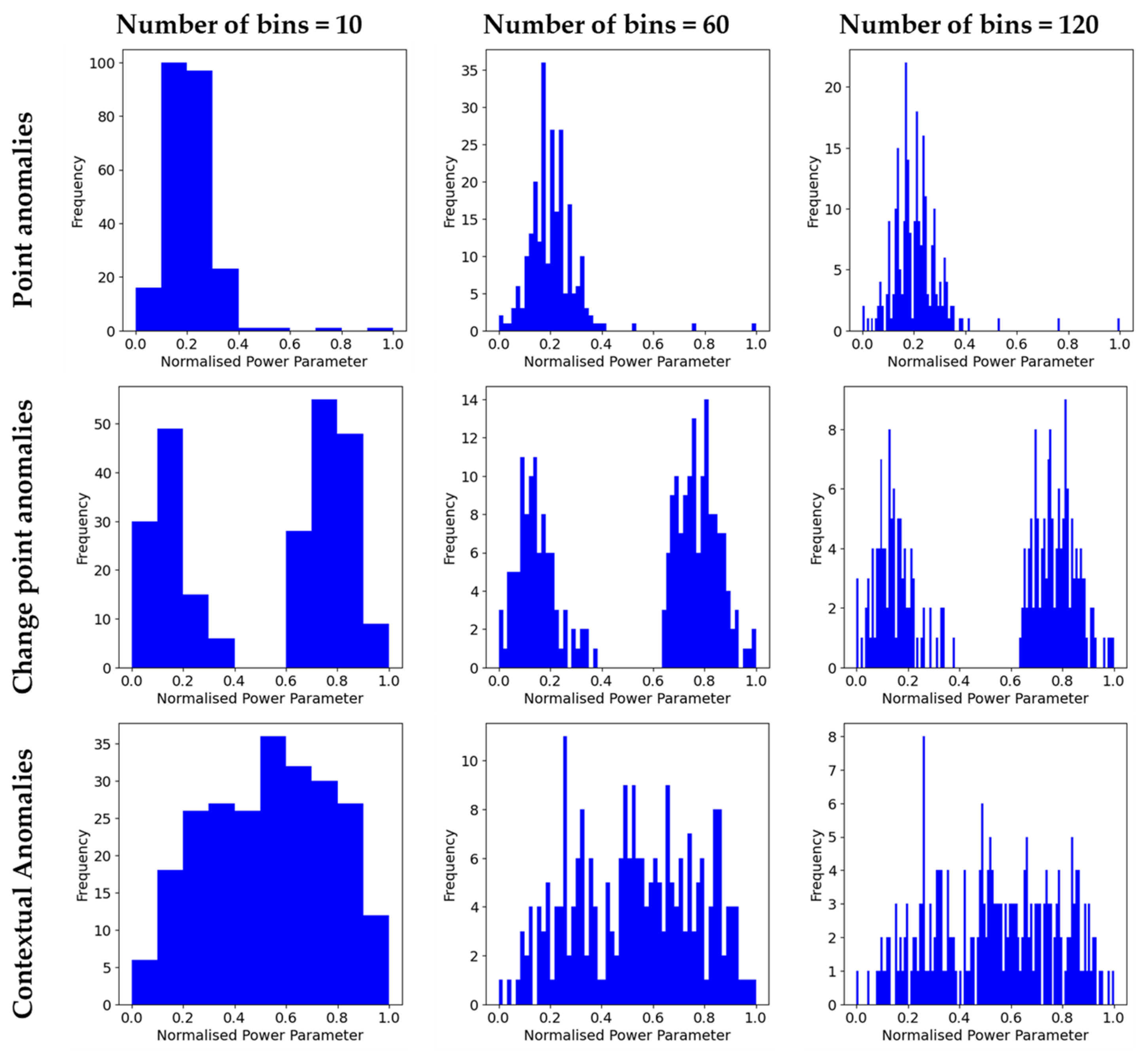
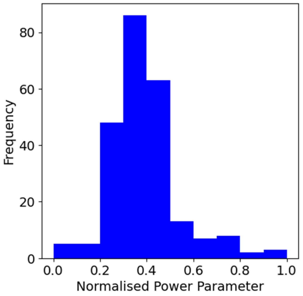
The data pre-processing steps median centring and normalisation are also applied. Subsequently, the histograms are generated. As shown in Figure 5, clear differences can be identified for each type of anomaly. For instance, the histograms related to point anomalies tend to have isolated frequencies in higher bins, which relate to each of the point anomalies presented in the sequence. It can also be observed that these bins tend to have fewer frequencies compared to the bins that relate to the normal sequences, as the number of spikes presented in a sequence tends to be minimal. Consequently, the result is a histogram highly skewed to the right with a long tail toward higher values. Regarding the second type of anomalies, change point anomalies, a bimodal distribution can be perceived. This bimodal distribution occurs due to the two distinct operational states that occur in this type of sequence. Finally, the last type of anomaly, which relates to contextual anomalies, tends to present a unimodal histogram that is widely spread. Thus, by performing a visual inspection, one can identify that the histogram of spike anomalies tends to be highly skewed to the right, change point anomalies tend to present a bimodal distribution, and contextual anomalies tend to present a unimodal distribution that is widely spread. Therefore, the estimation of a similarity matrix that considers the similarity degree between a pair of histograms is expected to capture the similarity between sequences that present the same type of anomalies and the dissimilarity between sequences that present different types of anomalies.
Regarding the number of bins, it can be observed that with a reduced number of bins, the differences between types of anomalies can be captured. Thus, even though a higher number of bins can provide further information, as also perceived in Figure 5, it can also increase the computational cost of the model. Thus, a search space is defined to identify the lowest number of bins that facilitates the best results whilst attempting to reduce the complexity and computational cost of the model. The search space was set to [2, 240], 240 being the length of the sequence. The best results are obtained when the number of bins considered is 5.
Once all histograms are generated, the similarity matrix is estimated, which encompasses the similarity degree between each pair of histograms. The resulting matrix is introduced as the input of the hierarchical clustering, where the centroid linkage is utilised. To evaluate the labels obtained from the hierarchical clustering, both the accuracy and the confusion matrix are estimated. The accuracy metric is considered, as it is probably the most popular metric utilised when addressing a multi-class classification task. To estimate the accuracy, the following equation is considered:
a c c u r a c y = T P + T N T P + T N + F P + F N .
Regarding the confusion matrix, it can be defined as a cross table that describes the number of occurrences between two rates: true (actual) classifications and predicted classifications. A graphical representation of a confusion matrix is shown in Figure 6.
Additionally, the macro precision, macro recall, macro F1, Matthews correlation coefficient, Cohen’s Kappa coefficient, and average execution time are estimated. The macro precision and macro recall are estimated by utilising Equations (9) and (10), respectively.
M a c r o   A v e r a g e   P r e c i s i o n   ( M A P ) = 1 K i = 1 K p r e c i s i o n i ,
M a c r o   A v e r a g e   R e c a l l   M A R = 1 K i = 1 K r e c a l l i ,
where K is the number of classes, precision equals to T P T P + F P , and recall equals to T P T P + F N . By determining the macro average precision and macro average recall, the macro F1 can be estimated as indicated by Equation (11).
M a c r o   F 1 = 2 × M A P × M A R M A P + M A R .
The Matthews correlation coefficient (MCC) can be defined as follows:
M C C = c × s k K p k × t k s 2 k K p k 2 s 2 k K t k 2 ,
where:
c = k K C k k is the total number of correctly predicted elements,
s = i K j K C i j is the total number elements,
p k = i K C i k is the number of times that class k was predicted,
t k = i K C k i is the number of times that class k truly occurred.
Finally, Cohen’s Kappa coefficient (K) is calculated by utilising Equation (13).
K = c × s k K p k × t k s 2 k K p k × t k
Despite the fact that the proposed model performs clustering, classification metrics can be applied due to the manual labelling of the injected anomalies. The accuracy of the model is 95.20%. As Figure 7 shows, 2304 instances were accurately classified. The model suggested that the most optimal number of clusters for this case study is four, rather than the initially anticipated three (point anomalies, change point anomalies, and contextual anomalies). This is because certain sequences exhibited high variability, which made it challenging to differentiate between contextual and change point anomalies. The additional cluster is marked as red in the resulting confusion matrix (XX). A total of 49 sequences were clustered into this additional group. Additionally, 67 sequences were misclassified, with point anomalies incorrectly labelled as contextual anomalies, and vice versa. These misclassifications are attributed to the high variability of certain sequences containing point anomalies, which can be easily confused with contextual anomalies.
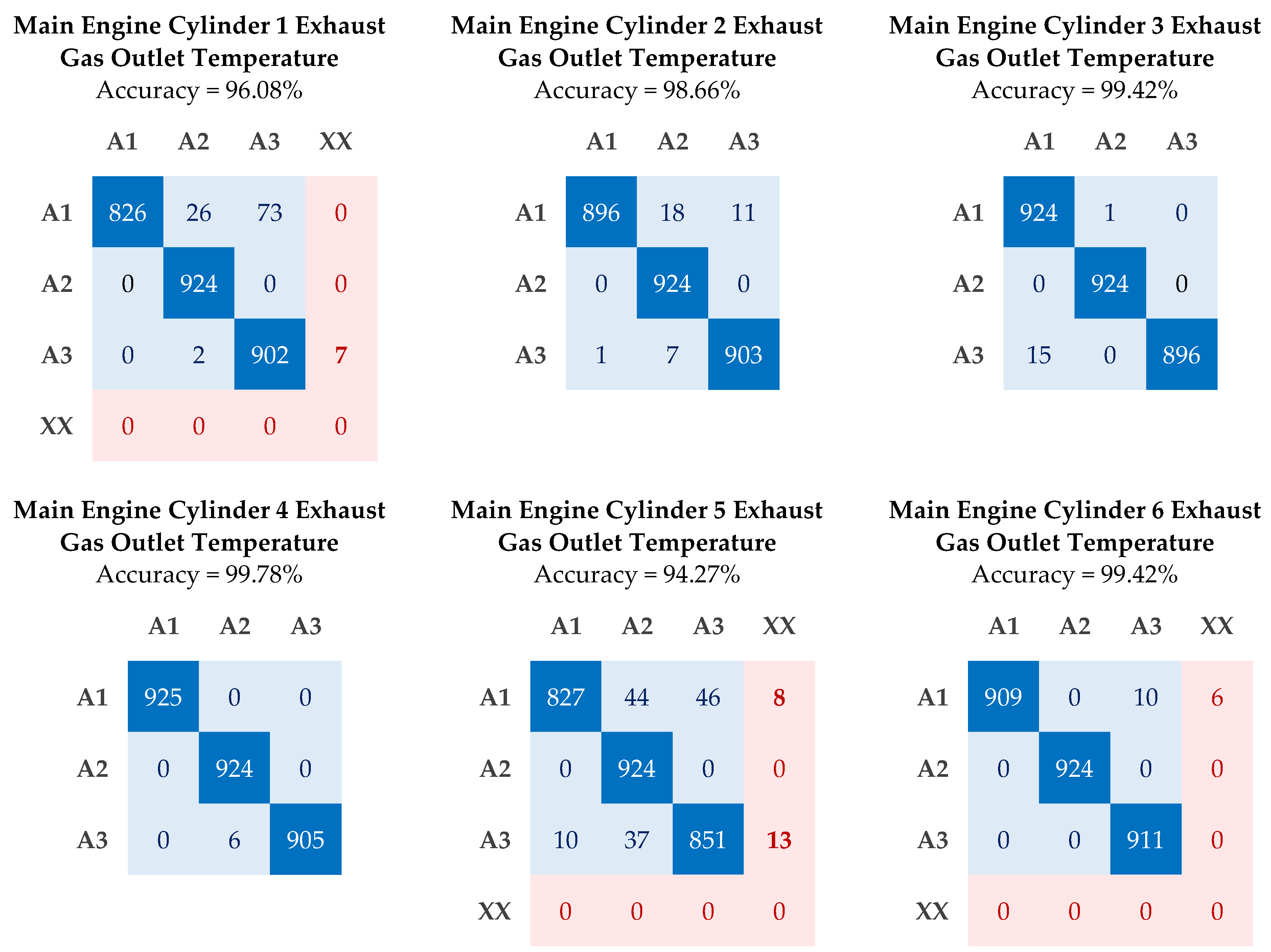
To complement the above results, an additional six parameters are explored. Specifically, the exhaust gas outlet temperatures of each of the six main engine cylinders are analysed. Analogous to the main engine power parameter, the proposed methodology effectively differentiates among the three distinct types of anomalies. As observed in Figure 8, the minimum accuracy, which is 94.27%, is obtained when analysing the exhaust gas outlet temperature of cylinder 5. In contrast, the maximum accuracy, which is 99.78%, is achieved when cylinders 4 and 6 are considered. The main results of this study are summarised in Table 2.
An additional case study is implemented to further analyse the following aspects:
  • The limited number of faults. Faults can be considered rare events if compared to normal operations, as a fault during operational conditions may lead to an inadequate functioning of marine machinery. Thus, preventive actions are usually performed in advance to avert any fault that can jeopardise the operations of the systems. This results in a lack of fault data, which can limit most of the studies that utilise deep learning approaches, as they require significant amounts of data for training. For this reason, recent studies focus on data augmentation techniques. Nevertheless, this study aims to provide an alternative for the labelling of fault data based on histogram similarity and hierarchical clustering. While the first case study contained a significant amount of fault sequences (2420 sequences), the third case study considers a total of 35 anomaly sequences to analyse whether the proposed model is effective with a limited amount of fault data.
  • Fault imbalance. It is not uncommon when dealing with this type of case study that the different fault types exhibit varying frequencies. This is because certain fault types may occur more frequently than others, which can be rare. To validate whether the proposed model can handle fault imbalance, the model is tested using three types of anomaly sequences. The distribution of the anomaly sequences is as follows: 20 out of 35 anomaly sequences relate to point anomalies, 5 out of 35 relate to change point anomalies, and 10 out of 35 relate to contextual anomalies (please see Table 3 for further details).
  • Explainability. The proposed model considers hierarchical clustering to understand the classifications provided through the model based on the histogram similarity.
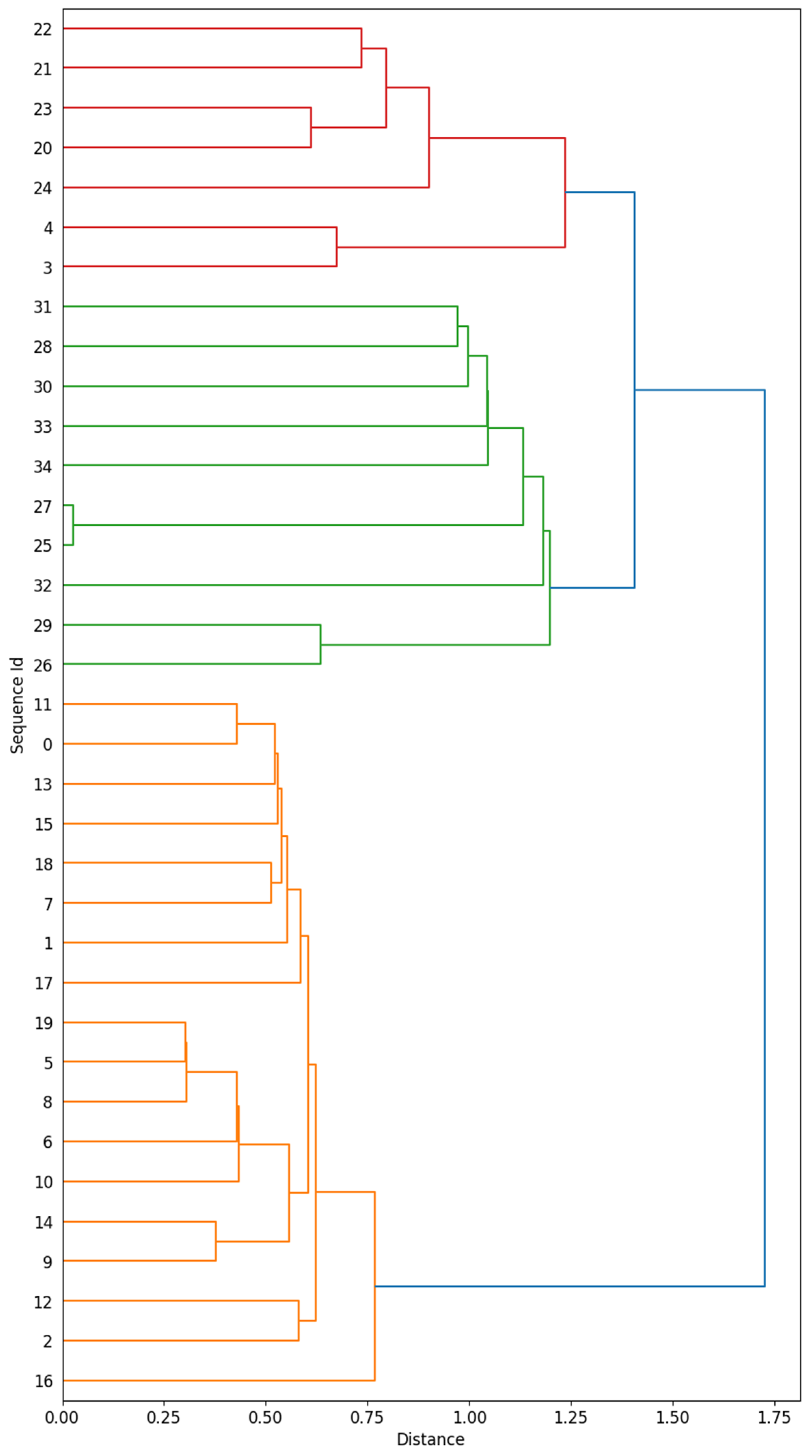
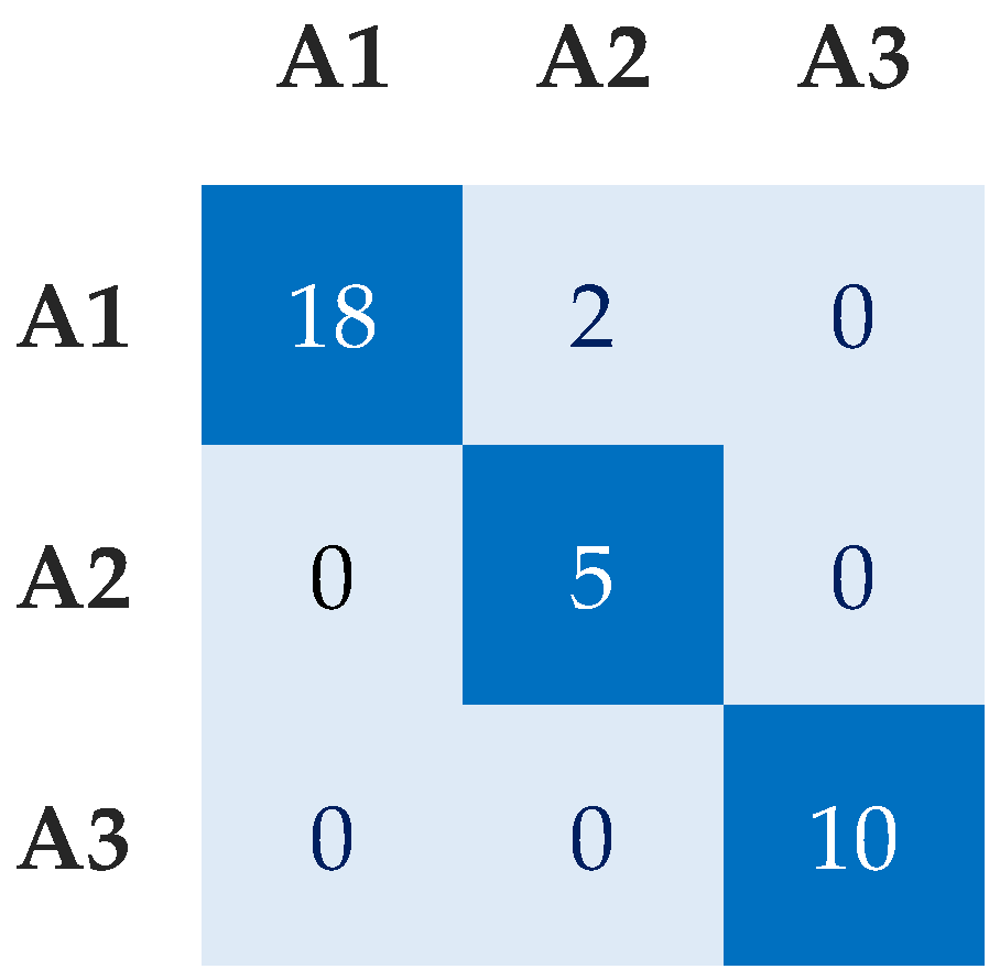
Figure 9 graphically presents the resulting dendrogram for the current case study. To enhance interpretability, single linkage was considered instead. As illustrated, the model successfully identifies the three distinct types of anomalies. The red labels refer to change point anomalies, the green labels to contextual anomalies, and the orange to the point anomalies. The analysis only reveals two misclassifications occurred, which relate to sequences 3 and 4, and were incorrectly categorised as change point anomalies instead of point anomalies. Consequently, the resulting accuracy for this case study is 94.29%. The confusion matrix can also be evaluated by consulting Figure 10.
The mentioned misclassification can be further analysed due to the explainability of the model. Firstly, the 3 and 4 sequences could be considered as a fourth independent cluster, as it can be perceived that they are not very similar to any of the other sequences. This can also be perceived with the sequences 26 and 29. For instance, if sequence 3 is graphically represented, as seen in Figure 11, the histogram is distinct to the ones indicated in Figure 5. Thus, it can be determined that this misclassification is related to the lack of similarity between sequences 3 and 4 and the remaining sequences. This difference relates to the high variability of the sequences, which fail to isolate the point anomalies presented.
Finally, to assess whether the proposed methodology can handle different types of faults than the ones presented in the previous case study, a new case study is introduced where the following type of fault patterns are considered: (1) drop (F1), (2) noise (F2), (3) exponential increase (F3), (4) sudden fluctuations (F4), and (5) stuck (F5). The drop pattern usually occurs when there is a loss of signal due to, for instance, power failure, physical disconnection, or sensor malfunction. Even though in these situations the result of these faults tends to be a drop to either 0 or a very low value, in this study, the fault is simulated in a way that the drop is not as abrupt. The second fault pattern refers to random noise that was added to the signal in order to simulate calibration issues with the sensor. The third fault pattern relates to exponential increase, which may occur due to signal malfunction. The fourth fault pattern aims to address unpredictable variations in the sensor readings due to, for instance, electrical interference or external disturbances. Finally, the fifth and last fault pattern occurs when the sensor’s output remains at a fixed value, which does not reflect the actual measurement of the signal. This can occur due to sensor malfunction or inadequate data imputation of missing values. A graphical representation of each of these simulated fault patterns is introduced in Figure 12, Figure 13, Figure 14, Figure 15, Figure 16 and Figure 17.
The first analysis performed in this case study evaluates the effectiveness of the proposed methodology in dealing with imbalanced data. The analysed scenarios and the corresponding balanced accuracy are shown in Table 4. As it can be observed, the model’s performance of the model is not affected by data imbalance until the percentage of one fault-type data, compared to the total number of normal instances, reaches 20%. However, the balanced accuracy obtained is indicative of good performance, obtaining values of 0.82 and 0.85 for the cases of 10% and 20%, respectively.
Furthermore, an additional analysis that considers a total of 800 sequences (160 sequences) for each fault type was conducted. In this instance, an accuracy of 92.89% was achieved. The confusion matrix of this analysis is introduced in Figure 18. The misclassifications primarily occur between F2 and F3, with a total of 51 sequences being misclassified. Additionally, a total of 6 F5 were incorrectly classified as F4. All sequences for F1 and F4 were classified correctly.
Thus, results indicate that the consideration of histogram similarity in tandem with hierarchical clustering can be an option for the identification and labelling of anomalies; specifically, when there is no previous indication of the type of anomalies. However, the limitations of the proposed methodology cannot be diminished. For instance, the fault patterns need to be captured by the generated histograms so that the model can be effective. In addition, it can be computationally expensive when dealing with high-dimensional data. Despite these challenges, this methodology was proposed to label sufficient data to subsequently perform supervised learning. In an attempt to enhance the proposed methodology based on the obtained results, the future work guidelines are indicated below.
  • Anomalies needed to be injected to validate the proposed methodology due to the lack of fault data. An implementation of a real-world case study is expected once fault data is available to the authors.
  • Additional key ship machinery parameters such as auxiliary engine cylinder pressure and temperature can be explored and trialled further.
  • Analogously, due to the lack of fault data, univariate analysis was performed. However, a multivariate analysis could also be performed, while then adapting the proposed methodology accordingly.
  • Utilise other histogram similarity methods to generate a more robust similarity matrix.
  • Develop an ensemble model that can be adapted to the dimensions and characteristics of the data.
  • The silhouette coefficient is suggested as a metric for identifying the optimal parameters. However, other coefficients need to be evaluated to create a more robust model.
  • Create a holistic framework where the proposed methodology is incorporated as a preceding step of a fault diagnosis tool.
  • Develop a more efficient method to reduce the computational cost, as the introduced agglomerative clustering approach has a complexity of O(n3), resulting in an average execution time of 35.59 s for the first case study.
  • Even though the model showed good performance when the data was imbalanced, this performance is reduced when the dataset is severely imbalanced. Therefore, further work needs to be conducted to ensure that the methodology can handle highly imbalanced datasets.
  • Develop a framework that integrates the developed methodology with a fault diagnosis model so that a fault diagnosis model can be trained and deployed when fault label data are missing in real industrial applications.

5. Conclusions

The lack of labelled data is still a major concern for the development of fault diagnosis and prognosis approaches within the shipping industry. Accordingly, further efforts are required in the preceding steps to ensure that fault data are available and adequately labelled. Specifically, when deep learning techniques are advancing in this area of knowledge; techniques that require vast amounts of data.
Consequently, this study proposes a methodology based on histogram similarity and hierarchical clustering. Special attention is given to selecting critical parameters for model performance, including the number of bins defining the histogram and the number of clusters. The silhouette coefficient is suggested as a metric for identifying the optimal parameters.
To highlight the performance of the proposed methodology, a case study on a main engine of the tanker vessel is introduced. Specifically, the power engine parameter and a total of three distinct types of anomalies are analysed. Results indicate that the proposed method is simple and effective, achieving an accuracy of approximately 95% for the introduced case study. The proposed method can work for different data distributions, when the dataset is not severely imbalanced, and when the characteristics of the faults are unknown. However, the method also presents several disadvantages, such as the dependency on adequately capturing fault patterns by the generated histogram.

Author Contributions

Conceptualisation, C.V.-G.; methodology, C.V.-G.; validation, I.L. and N.C.-M.; formal analysis, C.V.-G.; investigation, C.V.-G.; writing—original draft preparation, C.V.-G.; writing—review and editing, C.V.-G., I.L. and N.C.-M. All authors have read and agreed to the published version of the manuscript.

Funding

This research received no external funding.

Data Availability Statement

The data utilised for this study is confidential.

Conflicts of Interest

The authors declare no conflict of interest.

References

  1. Xu, Y.; Jiang, X.; Ke, W.; Zhu, Q.; He, Y.; Zhang, Y.; Wang, Z. A novel pattern classification integrated GLPP with improved AROMF for fault diagnosis. Process Saf. Environ. Prot. 2023, 171, 299–311. [Google Scholar] [CrossRef]
  2. Mou, M.; Zhao, X.; Liu, K.; Hui, Y. Variational autoencoder based on distributional semantic embedding and cross-modal reconstruction for generalized zero-shot fault diagnosis of industrial processes. Process Saf. Environ. Prot. 2023, 177, 1154–1167. [Google Scholar] [CrossRef]
  3. Zhang, J.; Zhang, M.; Feng, Z.; Ruifang, L.V.; Lu, C.; Dai, Y.; Dong, L. Gated recurrent unit-enhanced deep convolutional neural network for real-time industrial process fault diagnosis. Process Saf. Environ. Prot. 2023, 175, 129–149. [Google Scholar] [CrossRef]
  4. Liu, J.; Hou, L.; He, S.; Zhang, X.; Yu, Q.; Yang, K.; Li, Y. Two-dimensional explainability method for fault diagnosis of fluid machine. Process Saf. Environ. Prot. 2023, 178, 1148–1160. [Google Scholar] [CrossRef]
  5. Galar, D.; Kumar, U. Diagnosis. In eMaintenance; Elsevier: Amsterdam, The Netherlands, 2017; pp. 235–310. [Google Scholar] [CrossRef]
  6. Dai, Y.; Qiu, Y.; Feng, Z. Research on faulty antibody library of dynamic artificial immune system for fault diagnosis of chemical process. In Computer Aided Chemical Engineering; Elsevier: Amsterdam, The Netherlands, 2018; pp. 493–498. [Google Scholar] [CrossRef]
  7. Xia, J.; Huang, R.; Chen, Z.; He, G.; Li, W. A novel digital twin-driven approach based on physical-virtual data fusion for gearbox fault diagnosis. Reliab. Eng. Syst. Saf. 2023, 240, 109542. [Google Scholar] [CrossRef]
  8. Wang, B.; Zhang, M.; Xu, H.; Wang, C.; Yang, W. A cross-domain intelligent fault diagnosis method based on deep subdomain adaptation for few-shot fault diagnosis. Appl. Intell. 2023, 53, 24474–24491. [Google Scholar] [CrossRef]
  9. Yin, M.; Li, J.; Li, H. A CNN approach based on correlation metrics to chemical process fault classifications with limited labelled data. Can. J. Chem. Eng. 2023, 101, 3982–3997. [Google Scholar] [CrossRef]
  10. Huang, H.; Wang, R.; Zhou, K.; Ning, L.; Song, K. CausalViT: Domain generalization for chemical engineering process fault detection and diagnosis. Process Saf. Environ. Prot. 2023, 176, 155–165. [Google Scholar] [CrossRef]
  11. Safaei, M.; Soleymani, S.A.; Safaei, M.; Chizari, H.; Nilashi, M. Deep learning algorithm for supervision process in production using acoustic signal. Appl. Soft Comput. 2023, 146, 110682. [Google Scholar] [CrossRef]
  12. Liu, H. Application of industrial Internet of things technology in fault diagnosis of food machinery equipment based on neural network. Soft Comput. 2023, 27, 9001–9018. [Google Scholar] [CrossRef]
  13. Yang, C.; Ma, S.; Han, Q. Robust discriminant latent variable manifold learning for rotating machinery fault diagnosis. Eng. Appl. Artif. Intell. 2023, 126, 106996. [Google Scholar] [CrossRef]
  14. Wang, R.; Huang, W.; Lu, Y.; Zhang, X.; Wang, J.; Ding, C.; Shen, C. A novel domain generalization network with multidomain specific auxiliary classifiers for machinery fault diagnosis under unseen working conditions. Reliab. Eng. Syst. Saf. 2023, 238, 109463. [Google Scholar] [CrossRef]
  15. Yang, C.; Ma, S.; Han, Q. Unified discriminant manifold learning for rotating machinery fault diagnosis. J. Intell. Manuf. 2023, 34, 3483–3494. [Google Scholar] [CrossRef]
  16. Jieyang, P.; Kimmig, A.; Dongkun, W.; Niu, Z.; Zhi, F.; Jiahai, W.; Liu, X.; Ovtcharova, J. A systematic review of data-driven approaches to fault diagnosis and early warning. J. Intell. Manuf. 2023, 34, 3277–3304. [Google Scholar] [CrossRef]
  17. Balaji, P.A.; Sugumaran, V. Comparative study of machine learning and deep learning techniques for fault diagnosis in suspension system. J. Braz. Soc. Mech. Sci. Eng. 2023, 45, 215. [Google Scholar] [CrossRef]
  18. Karatuğ, Ç.; Arslanoğlu, Y. Development of condition-based maintenance strategy for fault diagnosis for ship engine systems. Ocean Eng. 2022, 256, 111515. [Google Scholar] [CrossRef]
  19. Wang, R.; Chen, H.; Guan, C.; Gong, W.; Zhang, Z. Research on the fault monitoring method of marine diesel engines based on the manifold learning and isolation forest. Appl. Ocean Res. 2021, 112, 102681. [Google Scholar] [CrossRef]
  20. Ellefsen, A.L.; Han, P.; Cheng, X.; Holmeset, F.T.; Aesoy, V.; Zhang, H. Online Fault Detection in Autonomous Ferries: Using Fault-type Independent Spectral Anomaly Detection. IEEE Trans. Instrum. Meas. 2020, 69, 8216–8225. [Google Scholar] [CrossRef]
  21. Tan, Y.; Zhang, J.; Tian, H.; Jiang, D.; Guo, L.; Wang, G.; Lin, Y. Multi-label classification for simultaneous fault diagnosis of marine machinery: A comparative study. Ocean Eng. 2021, 239, 109723. [Google Scholar] [CrossRef]
  22. Lei, Y. Individual intelligent method-based fault diagnosis. In Intelligent Fault Diagnosis and Remaining Useful Life Prediction of Rotating Machinery; Elsevier: Amsterdam, The Netherlands, 2017; pp. 67–174. [Google Scholar] [CrossRef]
  23. Zhong, B.; Zhao, M.; Wang, L.; Fu, S.; Zhong, S. DCSN: Focusing on hard samples mining in small-sample fault diagnosis of marine engine. Measurement 2024, 235, 114929. [Google Scholar] [CrossRef]
  24. Guo, Y.; Zhang, J.; Sun, B.; Wang, Y. A universal fault diagnosis framework for marine machinery based on domain adaptation. Ocean Eng. 2024, 302, 117729. [Google Scholar] [CrossRef]
  25. Xiao, G.; Wang, Y.; Wu, R.; Li, J.; Cai, Z. Sustainable Maritime Transport: A Review of Intelligent Shipping Technology and Green Port Construction Applications. J. Mar. Sci. Eng. 2024, 12, 1728. [Google Scholar] [CrossRef]
  26. Chen, X.; Ma, D.; Liu, R.W. Application of Artificial Intelligence in Maritime Transportation. J. Mar. Sci. Eng. 2024, 12, 439. [Google Scholar] [CrossRef]
  27. Ren, X.; Guo, Y.; Gong, Y. Fault diagnosis study of ship solar photovoltaic power generation system. J. Phys. Conf. Ser. 2024, 2771, 012024. [Google Scholar] [CrossRef]
  28. Liu, Z.; Yang, X.; Xie, Y.; Wu, M.; Li, Z.; Mu, W.; Liu, G. Multi-sensor cross-domain fault diagnosis method for leakage of ship pipeline valves. Ocean Eng. 2024, 299, 117211. [Google Scholar] [CrossRef]
  29. Lu, B.; Dibaj, A.; Gao, Z.; Nejad, A.R.; Zhang, Y. A class-imbalance-aware domain adaptation framework for fault diagnosis of wind turbine drivetrains under different environmental conditions. Ocean Eng. 2024, 296, 116902. [Google Scholar] [CrossRef]
  30. Velasco-Gallego, C.; De Maya, B.N.; Molina, C.M.; Lazakis, I.; Mateo, N.C. Recent advancements in data-driven methodologies for the fault diagnosis and prognosis of marine systems: A systematic review. Ocean Eng. 2023, 284, 115277. [Google Scholar] [CrossRef]
  31. Wang, R.; Chen, H.; Guan, C. DPGCN Model: A Novel Fault Diagnosis Method for Marine Diesel Engines Based on Imbalanced Datasets. IEEE Trans. Instrum. Meas. 2023, 72, 3504011. [Google Scholar] [CrossRef]
  32. Zhong, K.; Li, J.; Wang, J.; Han, M. Fault Detection for Marine Diesel Engine Using Semi-supervised Principal Component Analysis. In Proceedings of the 2019 9th International Conference on Information Science and Technology (ICIST), Hulunbuir, China, 2–5 August 2019; pp. 146–151. [Google Scholar] [CrossRef]
  33. Su, Y.; Gan, H.; Ji, Z. Research on Multi-Parameter Fault Early Warning for Marine Diesel Engine Based on PCA-CNN-BiLSTM. J. Mar. Sci. Eng. 2024, 12, 965. [Google Scholar] [CrossRef]
  34. Cheliotis, M.; Lazakis, I.; Theotokatos, G. Machine learning and data-driven fault detection for ship systems operations. Ocean Eng. 2020, 216, 107968. [Google Scholar] [CrossRef]
  35. Xu, F.; Jia, S.; Qu, C.; Chen, D.; Ma, L. Diesel Engine Fault Diagnosis Based on Convolutional Autoencoder Using Vibration Signals. Autom. Control. Comput. Sci. 2024, 58, 185–194. [Google Scholar] [CrossRef]
  36. Wu, H.; Jiang, R.; Wu, X.; Chen, X.; Liu, T. Marine Diesel Engine Fault Detection Based on Xilinx ZYNQ SoC. Appl. Sci. 2024, 14, 5152. [Google Scholar] [CrossRef]
  37. Wang, J.; Cao, H.; Cui, Z.; Ai, Z.; Jiang, K. Intelligent Fault Diagnosis of Marine Diesel Engines Based on Efficient Channel Attention-Improved Convolutional Neural Networks. Processes 2023, 11, 3360. [Google Scholar] [CrossRef]
  38. Zhu, G.; Huang, L.; Yin, J.; Gai, W.; Wei, L. Multiple faults diagnosis for ocean-going marine diesel engines based on different neural network algorithms. Sci. Prog. 2023, 106, 00368504231212765. [Google Scholar] [CrossRef] [PubMed]
  39. Pająk, M.; Kluczyk, M.; Muślewski, Ł.; Lisjak, D.; Kolar, D. Ship Diesel Engine Fault Diagnosis Using Data Science and Machine Learning. Electronics 2023, 12, 3860. [Google Scholar] [CrossRef]
  40. Guo, Y.; Zhang, J. Fault Diagnosis of Marine Diesel Engines under Partial Set and Cross Working Conditions Based on Transfer Learning. J. Mar. Sci. Eng. 2023, 11, 1527. [Google Scholar] [CrossRef]
  41. Shi, Q.; Hu, Y.; Yan, G. Hierarchical Multiscale Fluctuation Dispersion Entropy for Fuel Injection System Fault Diagnosis. Pol. Marit. Res. 2023, 30, 98–111. [Google Scholar] [CrossRef]
  42. Gokcek, V.; Genc, Y.; Kocak, G. Condition Monitoring and Fault Diagnosis of a Marine Diesel Engine with Machine Learning Techniques. Pomorstvo 2023, 37, 32–46. [Google Scholar] [CrossRef]
  43. Zhao, Y.; Wang, S.; Chen, N. Thermal fault diagnosis of marine diesel engine based on LSTM neural network algorithm. Vibroengineering Procedia 2022, 41, 198–203. [Google Scholar] [CrossRef]
  44. Yang, M.; Chen, H.; Guan, C. Research on diesel engine fault diagnosis method based on machine learning. In Proceedings of the 2022 4th International Conference on Frontiers Technology of Information and Computer (ICFTIC), Qingdao, China, 2–4 December 2022; pp. 1078–1082. [Google Scholar] [CrossRef]
  45. Chu, Z.; Gu, Z.; Chen, Y.; Zhu, D.; Tang, J. A Fault Diagnostic Approach for Underwater Thrusters Based on Generative Adversarial Network. IEEE Trans. Instrum. Meas. 2024, 73, 3524614. [Google Scholar] [CrossRef]
  46. Ai, Z.; Cao, H.; Wang, M.; Yang, K. Ship Ballast Water System Fault Diagnosis Method Based on Multi-Feature Fusion Graph Convolution. J. Phys. Conf. Ser. 2024, 2755, 012028. [Google Scholar] [CrossRef]
  47. Xu, X.; Lin, Y.; Ye, C. Fault diagnosis of marine machinery via an intelligent data-driven framework. Ocean Eng. 2023, 289, 116302. [Google Scholar] [CrossRef]
  48. Ai, Z.; Cao, H.; Wang, J.; Cui, Z.; Wang, L.; Jiang, K. Research Method for Ship Engine Fault Diagnosis Based on Multi-Head Graph Attention Feature Fusion. Appl. Sci. 2023, 13, 12421. [Google Scholar] [CrossRef]
  49. Zhengjie, L.; Xiaohui, Y.; Mengmeng, W.; Weilei, M.; Guijie, L. Leveraging deep learning techniques for ship pipeline valve leak monitoring. Ocean Eng. 2023, 288, 116167. [Google Scholar] [CrossRef]
  50. Wang, L.; Cao, H.; Cui, Z.; Ai, Z. A Fault Diagnosis Method for Marine Engine Cross Working Conditions Based on Transfer Learning. J. Mar. Sci. Eng. 2024, 12, 270. [Google Scholar] [CrossRef]
  51. Zhang, Y.; Han, D.; Shi, P. Semi-supervised prototype network based on compact-uniform-sparse representation for rotating machinery few-shot class incremental fault diagnosis. Expert Syst. Appl. 2024, 255, 124660. [Google Scholar] [CrossRef]
  52. Wu, Z.; Xu, R.; Luo, Y.; Shao, H. A holistic semi-supervised method for imbalanced fault diagnosis of rotational machinery with out-of-distribution samples. Reliab. Eng. Syst. Saf. 2024, 250, 110297. [Google Scholar] [CrossRef]
  53. Velasco-Gallego, C.; Lazakis, I. A real-time data-driven framework for the identification of steady states of marine machinery. Appl. Ocean Res. 2022, 121, 103052. [Google Scholar] [CrossRef]
  54. Dalheim, Ø.Ø.; Steen, S. Preparation of in-service measurement data for ship operation and performance analysis. Ocean Eng. 2020, 212, 107730. [Google Scholar] [CrossRef]
  55. Dalheim, Ø.Ø.; Steen, S. A computationally efficient method for identification of steady state in time series data from ship monitoring. J. Ocean Eng. Sci. 2020, 5, 333–345. [Google Scholar] [CrossRef]
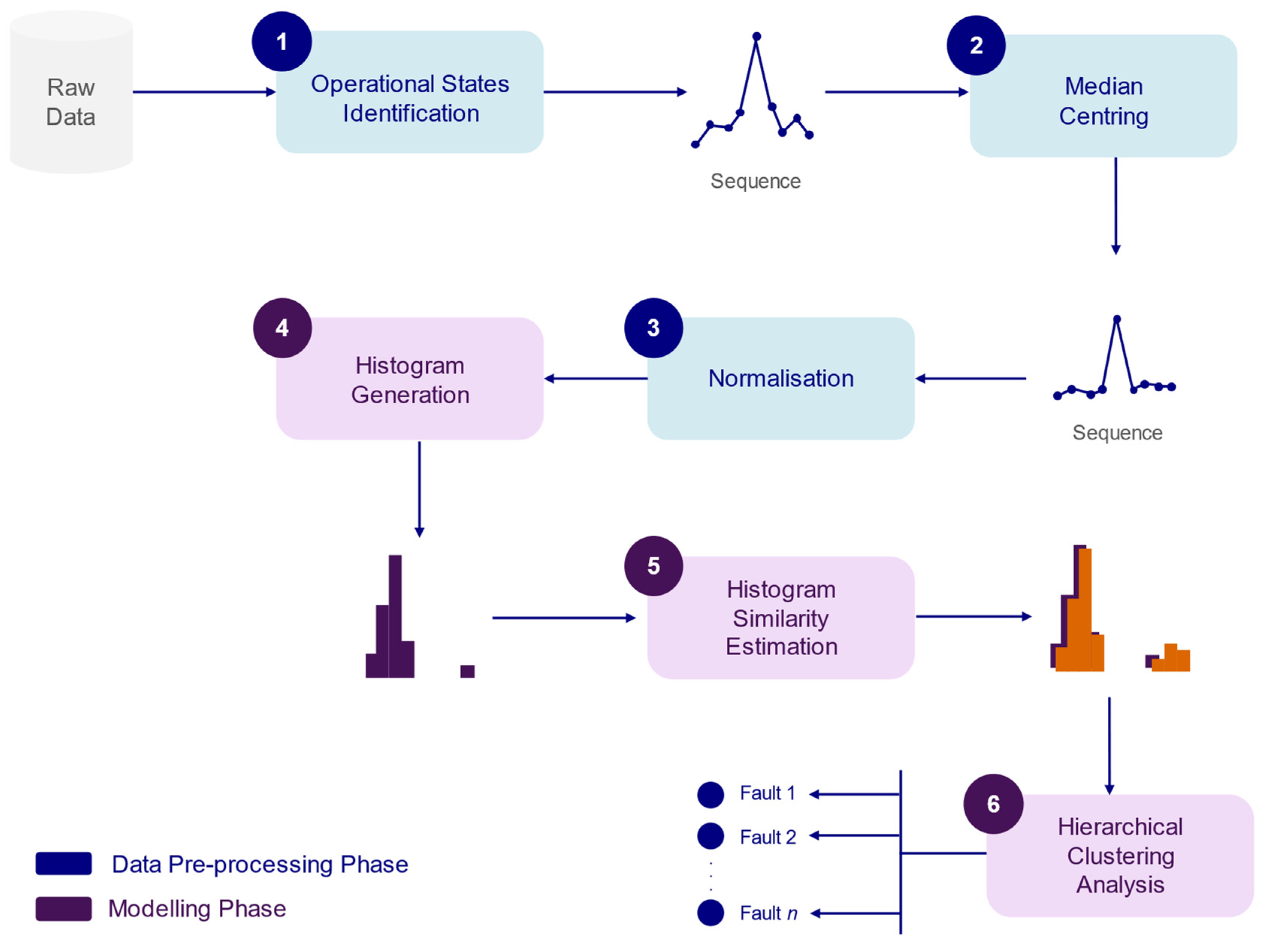
Figure 1. Graphical representation of the proposed methodology.
Jmse 12 01792 g001
Figure 2. Example of sequence with point anomalies due to potential operational, mechanical, environmental, or sensor-related issues.
Jmse 12 01792 g002
Figure 3. Example of sequence with change point anomalies due to changes in operating conditions.
Jmse 12 01792 g003
Figure 4. Example of sequence with contextual anomalies due to potential gradual deterioration of components, operational changes, or environmental influences.
Jmse 12 01792 g004
Figure 5. Example of histogram generation.
Jmse 12 01792 g005
Figure 6. Confusion matrix for multi-class classification with a total of n classes. The estimation of true positive (TP), true negative (TN), false positive (FP), and false negative (FN) is presented when considering a class k (0 ≤ kn).
Jmse 12 01792 g006
Figure 7. Confusion matrix of the first case study presented.
Jmse 12 01792 g007
Figure 8. Confusion matrix of the second case study presented.
Jmse 12 01792 g008
Figure 9. Dendrogram with clustering results.
Jmse 12 01792 g009
Figure 10. Confusion matrix of the third case study presented.
Jmse 12 01792 g010
Figure 11. Histogram of sequence 3 of the third case study.
Jmse 12 01792 g011
Figure 12. Example of a normal sequence.
Jmse 12 01792 g012
Figure 13. Example of a drop fault sequence, which may occur due to a loss of signal, for instance.
Jmse 12 01792 g013
Figure 14. Example of a noisy sequence, which may occur due to calibration issues of the sensor.
Jmse 12 01792 g014
Figure 15. Example of a sequence with exponential increase, which may occur due to stuck-at-faults issues.
Jmse 12 01792 g015
Figure 16. Example of a random fluctuations, which may occur due to unpredictable variations in the environment.
Jmse 12 01792 g016
Figure 17. Example of a sequence with a stuck value, which may occur due an inadequate data imputation performance or sensor malfunction.
Jmse 12 01792 g017
Figure 18. Confusion matrix of the fifth case study presented.
Jmse 12 01792 g018
Table 1. Categorisation of sequences of case study 1.
Type of AnomalyNumber of Instances% of Total
Point79933.0%
Change Point81133.5%
Contextual81033.5%
2420100.0%
Table 2. Main classification results for the first and second case study.
ParameterAccuracyMicro PrecisionMicro
Recall
Micro F1MCCKAverage
Execution Time
(s)
Power0.9520.9520.9520.9520.9300.92832.77
Cylinder 1 Exh. Gas Out. Temp.0.9600.9600.9600.9600.9400.94046.50
Cylinder 2 Exh. Gas Out. Temp.0.9860.9860.9860.9860.9800.97946.15
Cylinder 3 Exh. Gas Out. Temp.0.9940.9940.9940.9940.9910.99146.06
Cylinder 4 Exh. Gas Out. Temp.0.9970.9970.9970.9970.9960.99647.50
Cylinder 5 Exh. Gas Out. Temp.0.9420.9420.9420.9420.9100.91045.70
Cylinder 6 Exh. Gas Out. Temp.0.9940.9940.9940.9940.9960.99646.67
Table 3. Categorisation of sequences of case study 3.
Type of AnomalyNumber of Instances% of Total
Point2057%
Change point514%
Contextual1029%
35100.0%
Table 4. Performance of the proposed model based on the percentage of one fault type data compared to the total number of normal instances.
Percentage of One Fault Type Data Compared to the Total Number of Normal InstancesBalanced Accuracy
10%0.82
20%0.85
30%0.92
40%0.93
50%0.93
60%0.94
70%0.94
80%0.95
90%0.95
100%0.95
Disclaimer/Publisher’s Note: The statements, opinions and data contained in all publications are solely those of the individual author(s) and contributor(s) and not of MDPI and/or the editor(s). MDPI and/or the editor(s) disclaim responsibility for any injury to people or property resulting from any ideas, methods, instructions or products referred to in the content.