A Balanced Path-Following Approach to Course Change and Original Course Convergence for Autonomous Vessels

Abstract

This paper proposes a novel path-following method for autonomous ships that optimizes overall performance by balancing course changes and convergence to the original route. The proposed method extends the line-of-sight (LOS) guidance law by dynamically adjusting key parameters based on the ship’s cross-track error (XTE) and the distance of new course considering maneuvering characteristics. By incorporating these maneuvering characteristics, the method enables more precise adjustments during course changes, improving overall path-following performance. Simulation results showed that the proposed method outperformed three existing methods, including the traditional LOS guidance law, by minimizing overshoot and maintaining reasonable XTE during larger course changes. It achieved the lowest mean absolute cross-track error (MAE) while also significantly reducing the total time required to follow the path, highlighting its superior accuracy and efficiency in path following. These outcomes highlight the method’s potential to enhance significantly the path-following capabilities of autonomous vessels, contributing to greater efficiency and accuracy in pre-determined route navigation.

1. Introduction

Maritime autonomous surface ships (MASS) represent advanced technologies developed to improve maritime traffic efficiency and enhance safety. In recent years, considerable efforts have been directed toward the development of these technologies [1,2,3]. MASS are equipped with the ability to follow routes autonomously and adapt to surrounding environments without human intervention, through the integration of artificial intelligence (AI), sensor technologies, and navigation algorithms [4,5,6]. Key technologies enabling the generation of routes from the departure point to the destination, avoiding collision risks, and following the route are considered central to autonomous navigation [7,8,9]. Although various challenges and issues remain for the full implementation of autonomous ships, these technologies are anticipated to bring transformative changes to the maritime industry by reducing labor costs, minimizing accidents, and facilitating more efficient maritime traffic management [10,11].

Path following is one of the core technologies of MASS, aiming to ensure that a vessel follows a predefined path accurately. It involves real-time monitoring and adjustment of the vessel’s position, speed, and course angle to maintain the desired path. Path following at sea is particularly challenging due to environmental factors such as currents, waves, and wind, as well as the dynamic characteristics of the vessel [12]. Various algorithms have been proposed to address these complex challenges, with the line-of-sight (LOS) guidance law being widely used [13]. The traditional LOS guidance law operates by making the vessel follow a straight line between its current position and the target point, adjusting its heading angle accordingly [14,15]. However, the traditional LOS guidance law can be sensitive to environmental changes and may have limitations in situations requiring high precision.

Many researchers have proposed various algorithms to overcome the limitations of the traditional LOS guidance law [16]. Borhaug [17] suggested the integral LOS (ILOS) for underactuated marine vehicles in the presence of ocean currents, where the integral accumulates when external factors cause the vessel to deviate from its path, improving path-following performance even under challenging conditions. Lekkas [18] extended the ILOS by introducing a time-varying lookahead distance and demonstrated through simulations that the method performed well in tracking curved paths. Wan [19] further enhanced the ILOS by proposing a lookahead distance that varies as a function of the vessel’s speed and deviation distance, and validated the improvement through simulations with small unmanned surface vehicles (USVs), showing faster and more precise path-following performance without overshoot compared to the traditional ILOS. Han [20] introduced a method for selecting the lookahead distance in the ILOS guidance law based on fuzzy logic rules. He applied an algorithm to estimate the vessel’s state using an extended Kalman filter, rather than relying on an exact vessel model, and simulations demonstrated superior convergence to straight, curved, and turning paths compared to existing algorithms.

Additionally, Fossen [21] proposed the adaptive integral LOS (ALOS), which estimates and compensates for the sideslip caused by wind, waves, and currents. Simulations verified that even in the presence of unknown environmental disturbances, the vessel could correctly follow the path by estimating the sideslip. Liu [22] improved the traditional ALOS by introducing two predictors to estimate unknown sideslip angles, proposing the predictor-based LOS (PLOS). In another study [23], a reduced-order extended state observer (ESO) was introduced to accurately estimate and compensate for sideslip caused by unknown environmental disturbances in real time, resulting in the ESO-based LOS (ELOS). Nie [24] proposed the fuzzy adaptive ILOS (FAILOS), which incorporates a fuzzy logic system to estimate time-varying ocean currents and time-varying large sideslip angles, along with an adaptive fuzzy finite-time path following controllers to handle these variations.

Various path-following guidance laws, including the traditional guidance law, as well as ILOS, ALOS, PLOS, and ELOS, have garnered attention [25,26,27,28,29]. These guidance laws mainly focus on ensuring that, rather than following the entire path, the vessel can converge back to the original path when it deviates from a specific segment of the path. These methods also include additional functions to compensate for sideslip caused by wind, waves, and currents, but they still primarily focus on correcting deviations from the original path.

Typically, a vessel’s route is generally composed of straight segments connected by multiple waypoints; it is important not only to bring a vessel back to the original path when it deviates from a specific segment but also to ensure that the vessel stays as close as possible to the predefined route during course changes. Research aimed at following the entire route, including course changes, has also been conducted. Fossen [30] proposed a LOS guidance procedure that includes a projection algorithm and a waypoint switching algorithm to prevent the vessel from deviating excessively from the original route due to abrupt course changes when passing through waypoints. Moreira [31] introduced a minimum dynamic circle into the LOS guidance law to improve the vessel’s convergence back to the original path, and simulations were performed to track entire routes composed of multiple waypoints. Lekkas [32] proposed an LOS-based guidance law that dynamically adjusts the lookahead distance according to the vessel’s deviation from the path and incorporates the path-tangential angle and velocity-path relative angle. Su [33] further improved the lookahead-based ILOS method by introducing a function that adjusts the advance steering distance, which was fixed in the traditional LOS guidance law, based on the vessel’s length and course change angle to reduce overshoot during course changes. Unlike previous studies that focused on simulating the vessel’s convergence back to the original path, this research performed simulations following the entire route composed of multiple waypoints, confirming a reduction in deviation during course changes.

Despite the introduction of various concepts to reduce overshoot during course changes, previous methods often relied solely on cross-track error (XTE) or course change angle for parameter setting, and they did not provide a clear method for setting parameters specific to individual vessels. To address this, the present study proposes a new path-following method to improve the path-following performance of autonomous vessels, particularly large vessels, from the point of departure to the destination. The proposed method, based on the traditional LOS guidance law, presents a method for setting the target heading angle of the vessel according to its maneuvering characteristics, as well as optimal parameters for ensuring accurate path-following during course changes. For the simulations, the 300,000-ton oil tanker KVLCC2 was used, and its movement was modeled using a 3-degree-of-freedom maneuvering modeling group (MMG) model. Simulations confirmed that the proposed path-following method can effectively follow the entire route.

This study contributes to improving the path-following performance of large vessels by proposing an optimal parameter setting method tailored to the vessel’s maneuvering characteristics. It addresses the limitations of previous studies by reducing path deviation and controlling overshoot during course changes, thereby enhancing overall path-following performance. The remainder of this paper is organized as follows. Section 2 introduces the vessel used for simulation, the mathematical model of its maneuvering motion, and the existing path-following theories. Section 3 presents the newly proposed balanced path-following approach, which improves convergence to the original course and minimizes overshoot during course changes. Section 4 validates the effectiveness of the proposed path-following method through simulation tests. Finally, Section 5 provides the conclusions and suggests directions for future research.

2. Preliminaries

2.1. Mathematical Model of Ship Maneuvering Motion

This subsection presents the ship’s maneuvering motion model using the MMG approach and provides details about the KVLCC2 vessel, a 300,000-ton oil tanker used in the simulations.

Figure 1 shows the coordinate system used in this study. The $X-Y$ plane lies on the still water surface, and the positive $Z$-axis points vertically downward, defining the space-fixed coordinate system $O-XYZ$. The origin of the ship-fixed coordinate system $o-xyz$ is at the center of the vessel, with the $x$-axis pointing towards the bow, the $y$-axis towards the starboard, and the positive $z$-axis pointing downward towards the keel. In this system, $\psi$ denotes the yaw angle, $\delta$ denotes the rudder angle, $\beta$ refers to the drift angle, $r$ is the yaw rate, and $u$ and $v_m$ are the components of speed along the $x$ and $y$ axes, respectively, with $U$ representing the overall speed derived from $u$ and $v_m$.

The vessel’s motion is expressed as six degrees of freedom, consisting of linear motions along the $x$, $y$, and $z$ axes, which are surge, sway, and heave, and rotational motions, which are roll, pitch, and yaw. However, when the vessel is not moving fast enough for wave effects to be significant, has a sufficiently large metacentric height, and the weight distribution of the vessel is uniform, the heave, roll, and pitch motions can be neglected. Therefore, under such conditions, the vessel’s movement can be expressed using only three degrees of freedom: surge, sway, and yaw [34].

The maneuvering modeling group (MMG) of the Japan Society of Naval Architects and Ocean Engineers proposed a modular mathematical model for maneuvering (MMG model), which considers the hydrodynamic forces acting on the vessel separately. The MMG model is widely used in ship maneuvering simulations due to its ability to reflect accurately nonlinear ship dynamics and hydrodynamic forces acting on the hull, rudder, and propeller. Additionally, it offers flexibility and standardization, making it adaptable to various ship types and experimental data for reliable simulations.

Various techniques based on the MMG model have been developed, and Yasukawa [35] proposed a standardized MMG method. In this method, the surge, sway, and yaw motions are expressed as the hydrodynamic forces exerted by the hull, propeller, and rudder, as described by Equations (1)–(3):

$$\left(m+m_x\right)\dot{u}-\left(m+m_y\right)v_{m}r-x_{G}m{r}^2=X_H+X_R+X_P$$

(1)

$$\left(m+m_y\right){\dot{v}}_m+\left(m+m_x\right)ur-x_{G}m\dot{r}=Y_H+X_R$$

(2)

$$\left(I_{zG}+x_G^{2}m+J_z\right)\dot{r}-x_{G}m\left({\dot{v}}_m+ur\right)=N_H+N_R$$

(3)

Here, $m$ represents the mass, $I_{zG}$ is the moment of inertia about the vessel’s center of gravity, and $J_z$ is the added moment of inertia. The subscripts $H$, $R$, and $P$ represent the hull, rudder, and propeller, respectively, and the hydrodynamic forces acting on each are expressed as equations composed of hydrodynamic coefficients.

The hydrodynamic forces acting on the hull are represented by Equations (4)–(6). In these equations, $\rho$ is the water density, $L_{pp}$ is the length between perpendiculars, and $d$ is the draft of the vessel. The dimensionless lateral speed $v_m^{\prime }$ is defined as $v_m/U$, and the dimensionless yaw rate $r^{\prime }$ is defined as $r{L}_{pp}/U$. $X_H^{\prime }$ is expressed as the sum of the resistance coefficient $R_0^{\prime }$ and the quadratic and quartic polynomial functions of $v_m^{\prime }$ and $r^{\prime }$. $Y_H^{\prime }$ and $N_H^{\prime }$ are expressed as linear and cubic polynomial functions of $v_m^{\prime }$ and $r^{\prime }$ [35]:

$$X_H=\left(1/2\right)\rho L_{pp}d{U}^2{X}_H^{’}\left(v_m^{’}, r^{\prime }\right)$$

(4)

$$Y_H=\left(1/2\right)\rho L_{pp}d{U}^2{Y}_H^{’}\left(v_m^{’}, r^{\prime }\right)$$

(5)

$$N_H=\left(1/2\right)\rho L_{pp}^{2}d{U}^2{N}_H^{’}\left(v_m^{’}, r^{\prime }\right)$$

(6)

The hydrodynamic forces generated by the propeller are expressed by Equation (7), where $t_P$ is the thrust deduction factor, $n_P$ is the number of propeller revolutions per second, $D_P$ is the propeller diameter, $K_T$ is the thrust coefficient, and $J_P$ is the advance ratio of the propeller. $K_T$ is expressed as a quadratic polynomial function of $J_P$ [35]:

$$X_P=\left(1-t_P\right)\rho n_P^2{D}_P^4{K}_T\left(J_P\right)$$

(7)

The hydrodynamic forces generated by the rudder are expressed by Equations (8)–(10), where $t_R$, $a_H$, and $x_H$ are the hydrodynamic force coefficients due to the interaction between the rudder and the hull, $F_N$ is the rudder normal force, and $x_R$ represents the longitudinal coordinate of the rudder position [35]:

$$X_R=-\left(1-t_R\right)F_N\sin \delta$$

(8)

$$Y_R=-\left(1-a_H\right)F_N\cos \delta$$

(9)

$$X_R=-\left(x_R-a_H{x}_H\right)F_N\cos \delta$$

(10)

In this study, a very large crude carrier (VLCC) of 300,000 DWT, KVLCC2, was used for the simulation. The hydrodynamic coefficients and other related data of KVLCC2 are widely available through SIMMAN and previous studies [35,36,37], enabling precise modeling of the ship’s maneuvering motion using the MMG model. The abundance of the related research and data makes it easy to obtain the necessary information [38,39,40], and the large size of KVLCC2 aligns with the objective of this study, which is to analyze the path-following performance of large vessels.

Table 1. Main characteristics of KVLCC2.

Parameters	Values
$\mathrm{Length}\mathrm{between}\mathrm{perpendiculars}(L_{pp}$)	320.0 m
$\mathrm{Breadth}\left(B\right)$	58.0 m
$\mathrm{Draft}\left(d\right)$	20.8 m
$\mathrm{Displacement}(\nabla )$	312,600 m3
$\mathrm{Longitudinal}\mathrm{coordinate}\mathrm{of}\mathrm{center}\mathrm{of}\mathrm{gravity}\mathrm{of}\mathrm{ship}(x_G$)	11.2 m
$\mathrm{Block}\mathrm{coefficient}(C_b$)	0.810
$\mathrm{Propeller}\mathrm{diameter}(D_P$)	9.86 m
$\mathrm{Rudder}\mathrm{span}\mathrm{length}(H_R$)	15.80 m
$\mathrm{Profile}\mathrm{area}\mathrm{of}\mathrm{movable}\mathrm{part}\mathrm{of}\mathrm{mariner}\mathrm{rudder}(A_R$)	112.5 m2

shows the main particulars of the KVLCC2.

The main resistance coefficients, hydrodynamic coefficients, and rudder–propeller interaction coefficients for KVLCC2 are derived from previous studies [35,36,37].

Table 2. Hydrodynamic force coefficient of KVLCC2.

$X_{vv}^{\prime }$	−0.040	$Y_{vrr}^{\prime }$	−0.391	$m_x^{\prime }$	0.022	$C_2\left({\beta }_P>0\right)$	1.6
$X_{vr}^{\prime }$	0.002	$Y_{rrr}^{\prime }$	0.008	$m_y^{\prime }$	0.223	$C_2\left({\beta }_P<0\right)$	1.1
$X_{rr}^{\prime }$	0.011	$N_v^{\prime }$	−0.137	$J_z^{\prime }$	0.011	${\gamma }_R\left({\beta }_R>0\right)$	0.640
$X_{vvvv}^{\prime }$	0.771	$N_R^{\prime }$	−0.049	$t_P$	0.220	${\gamma }_R\left({\beta }_R<0\right)$	0.395
$Y_v^{\prime }$	−0.315	$N_{vvv}^{\prime }$	−0.030	$t_r$	0.387	$l_R^{\prime }$	−0.710
$Y_R^{\prime }$	0.083	$N_{vvr}^{\prime }$	−0.294	$a_H$	0.312	$\epsilon$	1.09
$Y_{vvv}^{\prime }$	−1.607	$N_{vrr}^{\prime }$	0.055	$x_H^{\prime }$	−0.464	$\kappa$	0.50
$Y_{vvr}^{\prime }$	0.379	$N_{rrr}^{\prime }$	−0.013	$C_1$	2.0	$f_{\alpha }$	2.747

shows the hydrodynamic coefficients of KVLCC2.

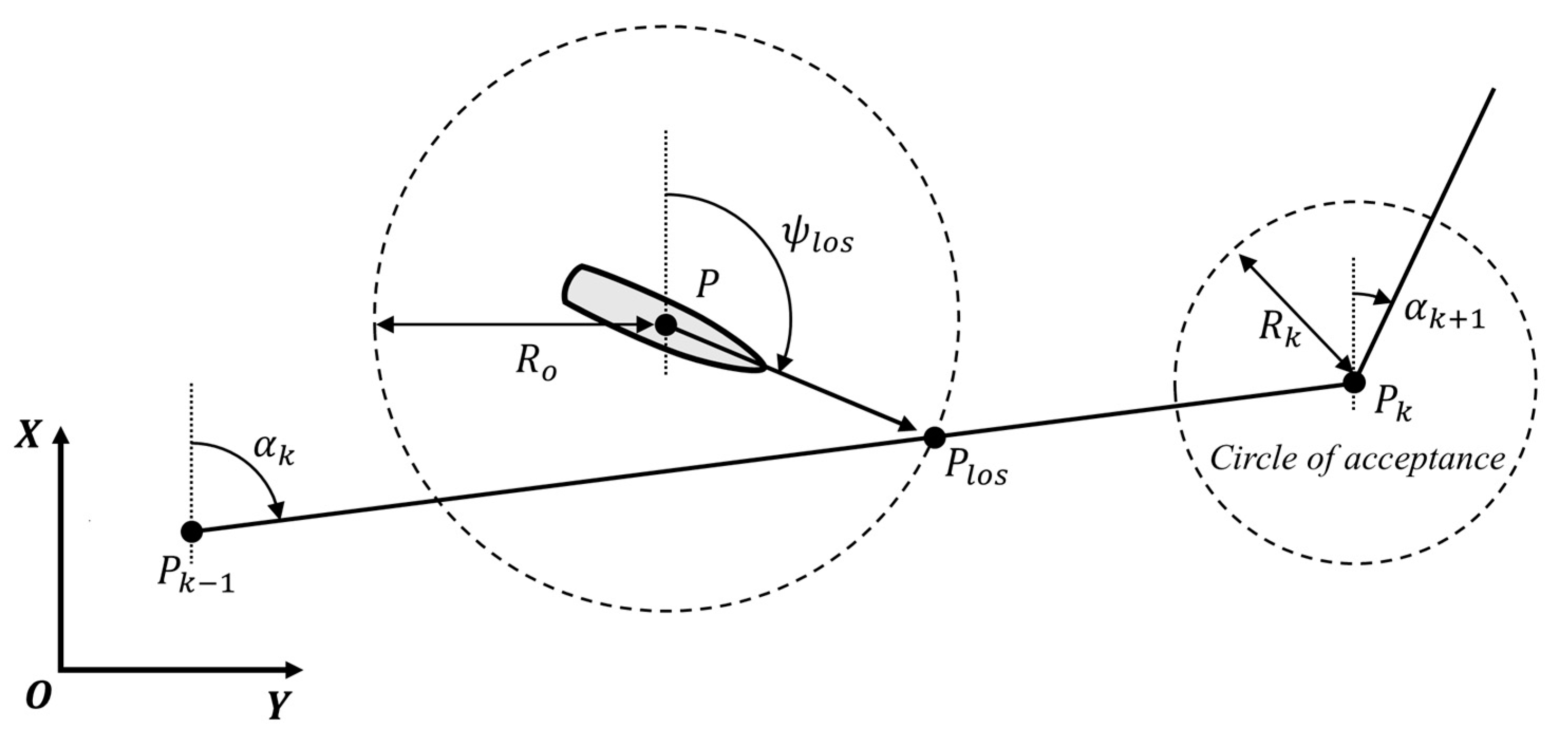
2.2. LOS Guidance Law

In this subsection, we address the theoretical aspects of the line-of-sight (LOS) guidance law and its variations, focusing on methods designed for following the entire path without considering external forces like sideslip. These theoretical foundations will serve as the basis for the new approach proposed in the following section, where the insights from this chapter will be referenced to introduce a novel path-following strategy.

2.2.1. Traditional LOS Guidance Law

The line-of-sight (LOS) guidance law is a concept primarily used in path guidance and control systems for mobile objects. It is particularly useful for underactuated systems, such as ships with limited steering capabilities, to adjust their direction and converge to a desired path while moving toward a target position. Figure 2 illustrates the basic principle of the traditional LOS guidance law [41].

In the traditional LOS guidance law, the ship follows the LOS point $P_{los}$, which lies on the straight segment connecting the previous waypoint $P_{k-1}\left(x_{k-1},y_{k-1}\right)$ and the current waypoint $P_k\left(x_k,y_k\right)$. When the ship’s current position is $P\left(x,y\right)$, the LOS angle ${\psi }_{los}$ can be calculated as follows [41]:

$${\psi }_{los}=\mathrm{atan}2\left({\displaystyle \frac{y_{los}-y}{x_{los}-x}}\right)$$

(11)

To position the LOS point on the original course, a virtual circle centered on the ship with a certain radius is considered. This circle intersects the straight segment connecting $P_{k-1}$ and $P_k$, and the intersection point closest to the next waypoint is designated as the LOS point. The LOS point can be calculated using the following formulas [41]:

$${\displaystyle \frac{y_{los}-y_{k-1}}{x_{los}-x_{k-1}}}={\displaystyle \frac{y_k-y_{k-1}}{x_k-x_{k-1}}}=\tan \left({\alpha }_k\right)$$

(12)

$${\left(x_{los}-x\right)}^2-{\left(y_{los}-y\right)}^2={R_o}^2$$

(13)

where ${\alpha }_k$ represents the original course angle, and $R_o$ is the radius of the circle centered on the ship. Generally, $R_o$ is set as a multiple of the ship’s length ($R_o=n{L}_{pp}$). Since the LOS point depends on both the previous and current waypoints, an algorithm is needed to switch between waypoints as the ship navigates. The waypoint is switched when the ship’s current position $P\left(x,y\right)$ enters the circle of acceptance around the current waypoint $P_k\left(x_k,y_k\right)$ [41]:

$${\left(x_k-x\right)}^2+{\left(y_k-y\right)}^2\le R_k^2$$

(14)

The radius of the circle of acceptance, $R_k$, is typically set as a multiple of the ship’s length. It is recommended that $R_k$ be smaller than or equal to the radius of the virtual circle around the ship, $R_o$ [30].

The traditional LOS guidance law is a simple and easy-to-implement algorithm that allows the vessel to follow a predefined path. However, it lacks clarity on how to set the parameters $R_o$ for calculating the LOS angle and $R_k$ for waypoint switching.

2.2.2. LOS Guidance Using Minimum Dynamic Circle

Moreira [31] improved upon the traditional LOS guidance law by modifying the previously fixed parameter $R_o$, which plays a critical role in determining the LOS position. The modification allowed $R_o$ to become a minimum dynamic circle value between two consecutive waypoints, thereby improving the convergence of the LOS algorithm.

Equation (15) provides the minimum circle, $d_{mdc}$. Here, $d_{pw}$ represents the distance between the vessel and the previous waypoint, $d_{cw}$ represents the distance between the vessel and the current waypoint, and $d_{bw}$ is the distance between the previous waypoint and the current waypoint [31]:

$$d_{mdc}=\sqrt{d_{pw}^2+{\left({\displaystyle \frac{d_{bw}^2-d_{cw}^2+d_{pw}^2}{2d_{bw}}}\right)}^2}$$

(15)

$$d_{pw}=\sqrt{{\left(x-x_{k-1}\right)}^2+{\left(y-y_{k-1}\right)}^2}$$

(16)

$$d_{cw}=\sqrt{{\left(x_k-x\right)}^2+{\left(y_k-y\right)}^2}$$

(17)

$$d_{bw}=\sqrt{{\left(x_k-x_{k-1}\right)}^2+{\left(y_k-y_{k-1}\right)}^2}$$

(18)

When $d_{cw}$ becomes 0 and $d_{pw}$ equals $d_{bw}$, $d_{mdc}$ also becomes 0, which must be avoided. To prevent this, $R_o$ is defined as follows [31]:

$$R_o=d_{mdc}+L_{pp}$$

(19)

This improves upon the traditional LOS guidance law, where $R_o$ is typically assumed to be $n{L}_{pp}$, with $n$ greater than 1. Thus, the LOS position is given by the following equation [31]:

$${\left(x_{los}-x\right)}^2-{\left(y_{los}-y\right)}^2={\left(d_{mdc}+L_{pp}\right)}^2$$

(20)

Although the LOS guidance using the minimum dynamic circle improved the convergence of the LOS algorithm by dynamically calculating $R_o$ based on the relationship between the vessel, the previous waypoint, and the current waypoint, it did not address the parameter $R_k$ necessary for appropriate waypoint shifting.

2.2.3. Time-Varying Lookahead Distance Guidance Law

Lekkas [32] improved upon the lookahead distance-based LOS guidance method originally proposed by Papoulias [42] to minimize deviation from the intended path. The proposed method dynamically adjusts the lookahead distance over time, allowing for smoother convergence to the given path. This dynamic adjustment enables faster convergence and ensures smooth path-following, even on routes with tight curvature. The method also demonstrates effective path-following performance in unstructured environments. Figure 3 illustrates the time-varying lookahead distance guidance law.

This method sets the LOS angle using the lookahead distance and the velocity-path relative angle, instead of calculating the LOS position ($P_{los}$) as in conventional methods. The velocity-path relative angle ensures that the velocity is aimed at a point on the original course that is located $\Delta >0$ ahead of the direct projection onto the original course.

The LOS angle can be calculated as shown in Equation (21), where ${\psi }_r$ represents the velocity-path relative angle and $\Delta$ denotes the lookahead distance. The minimum and maximum allowed values for $\Delta$, ${\Delta }_{min}$, and ${\Delta }_{max}$, respectively, are important design parameters, along with the convergence rate $\gamma >0$. The cross-track error (XTE) $d_e$, which represents the lateral deviation of the ship from the original course, is calculated using the ship’s current position $P\left(x,y\right)$, the current waypoint $P_k\left(x_k,y_k\right)$, and the original course angle ${\alpha }_k$ [32]:

$${\psi }_{los}={\alpha }_k+{\psi }_r$$

(21)

$${\psi }_r=-\mathrm{atan}2\left({\displaystyle \frac{d_e}{\Delta }}\right)$$

(22)

$$\Delta =\left({\Delta }_{max}+{\Delta }_{min}\right)e^{-\gamma \left|d_e\right|}+{\Delta }_{min}$$

(23)

$$d_e=-\left(x-x_k\right)\sin {\alpha }_k+\left(y-y_k\right)\cos {\alpha }_k$$

(24)

When the vessel is far from the original course, a smaller $\Delta$ value is assigned to induce more aggressive behavior that quickly reduces XTE. Conversely, when the vessel is close to the original course, a larger $\Delta$ value is used to prevent overshoot. Since the concepts of “far” and “close” are relative, various constraints, such as the ship’s maneuvering characteristics, must be considered when determining ${\Delta }_{min}$, ${\Delta }_{max}$, and $\gamma$.

Additionally, Su [33] pointed out that in the LOS guidance law using time-varying lookahead distance, $R_k$ is set as a fixed value, leading to overshoot and deviation during course changes. To address this issue, a strategy for adjusting $R_k$, based on the turning angle and the length of the ship, was proposed through numerous simulation experiments, as shown in Equation (25):

$$R_k=\left(3\left({\alpha }_{k+1}-{\alpha }_k\right)+1.5\right)L_{pp}$$

(25)

The traditional line-of-sight (LOS) guidance law and its variations have been reviewed. While the method for setting $R_o$ has become dynamic, allowing adjustments based on the extent of deviation from the path, it still only mentions the need to consider various conditions such as the ship’s maneuvering characteristics without fully incorporating these characteristics. Similarly, the method for setting $R_k$, which was previously based simply on a multiple of the ship’s length, has been improved to account for the turning angle, but it still does not fully reflect the ship’s maneuvering characteristics.

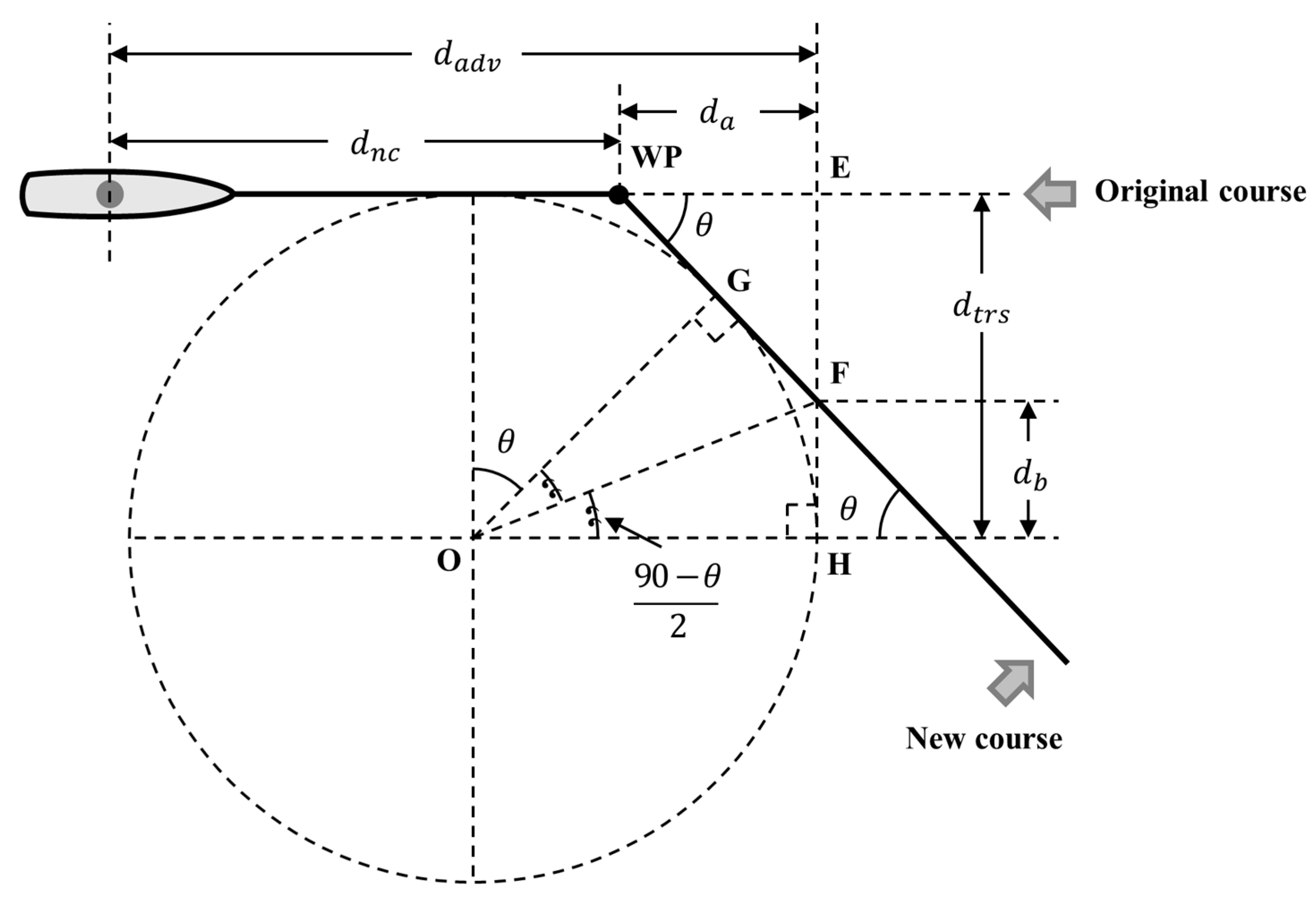
2.3. Distance of New Course Mathematical Model

Although many studies on path following and guidance have been conducted, most have focused on using the ship’s length and course change angle to set waypoint switching points. This subsection reviews a mathematical model for determining the new course distance based on the ship’s maneuvering characteristics, aiming to set $R_k$ in a way that minimizes overshoot and path deviation.

When changing course, a ship begins to change direction only after a certain distance has been covered in a straight line, even if the rudder is operated. To initiate a course change, the rudder must be activated before reaching the waypoint. The point where the rudder is activated is called the wheel over point (WOP), and the distance from the waypoint to the WOP is called the distance of new course.

If the distance of new course is not properly set, the rudder might be activated too early or too late, leading to significant deviations from the intended path during course changes. Therefore, the distance of new course must be determined by considering factors such as the angle between courses, the rudder angle used, the size and shape of the ship, its speed, maneuverability, and sea conditions.

Figure 4 illustrates the advance transfer mathematical model (ATMM) used to calculate the distance of new course by considering the course change angle and the advance and transfer distances at a 35° turning circle [43]. The distance of new course $d_{nc}$ when the course change angle is $\theta$, is calculated as the following:

$$d_{nc}=d_{adv}-d_a$$

(26)

where $d_{adv}$ is the advance distance. $d_a$ is calculated using the following equation:

$$d_a={\displaystyle \frac{\overline{EF}}{\tan \theta }}$$

(27)

Here, $\overline{EF}$ is calculated using the relationship: $\overline{EF}=d_{trs}-d_b$, where $d_{trs}$ is the transfer distance, and $d_b$ is calculated as follows:

$$d_b=d_{trs}\cdot \tan \angle FOH$$

(28)

According to the tangent segments theorem, from an external point $F$, the lengths of the tangent segments to the circle are equal, so $\overline{FG}=\overline{FH}$. Therefore, triangles $△FOH$ and $△FOG$ are congruent, leading to $\angle FOH=\angle FOG=\angle GOH/2$. Hence, $\angle FOH=\left(90-\theta \right)/2$. Substituting $d_b$ back into the equation for $d_a$, we get the following:

$$d_a={\displaystyle \frac{d_{trs}\left(1-\tan \left(\frac{90°-\theta }{2}\right)\right)}{\tan \theta }}$$

(29)

Finally, substituting $d_a$ back into the equation for $d_{nc}$, the distance of new course $d_{nc}$ is expressed as follows [43]:

$$d_{nc}=d_{adv}-{\displaystyle \frac{d_{trs}\left(1-\tan \left(\frac{90°-\theta }{2}\right)\right)}{\tan \theta }}$$

(30)

Since this formula calculates the new course distance based on the course change angle and the ship’s turning characteristics, using it to set the waypoint switching point is expected to minimize overshoot and path deviation during course changes in path following.

Figure 4. ATMM for calculating distance of new course.

Figure 4. ATMM for calculating distance of new course.

3. Balanced Path-Following Approach

Various LOS guidance methods are used for path following, but these methods mainly focus on ensuring that the vessel converges back to the original path when it deviates. However, waypoint switching is equally important for complete path following, yet it has not been thoroughly addressed. Furthermore, although these methods emphasize the need to set various parameters, such as $R_o$, in accordance with the ship’s characteristics, clear guidance on how to set these parameters is not sufficiently provided.

This section introduces the newly proposed balanced path-following approach for tracking an entire route composed of multiple waypoints. The focus is on how to set appropriately the parameters $R_o$ and $R_k$, which are essential for path-following, based on the ship’s maneuvering characteristics, course change angle, and XTE.

3.1. Waypoint Switching Point

When a waypoint is switched, the vessel must change its heading to align with the new course. The degree of difficulty in this transition depends on the course change angle between the original course and the new course. A larger course change angle means a longer distance is required for the vessel to complete the heading adjustment, from the turning point to the point where the heading is fully aligned with the new course. Conversely, when the course change angle is smaller, the distance needed for heading adjustment is correspondingly shorter.

In the traditional LOS guidance law, a fixed circle of acceptance is often used, where the waypoint switching occurs once the vessel enters this predefined circle. However, using a fixed circle cannot accommodate the varying conditions that arise from different course change angles, which could lead to overshoot or inefficient maneuvers. Therefore, a dynamic approach is necessary to adjust the circle of acceptance based on the specific course change angle.

In this study, the circle of acceptance $R_k$, which is necessary for setting the waypoint switching point, is dynamically calculated using the advance transfer mathematical model (ATMM). The ATMM takes into account the advance distance ($d_{adv}$) and transfer distance ($d_{trs}$) at the turning point, allowing the adjustment of $R_k$ as a function of the course change angle. Equation (31) shows how $R_k$ is computed based on the course change angle (${\alpha }_{k+1}-{\alpha }_k$) between the original and new courses:

$$R_k=d_{adv}-{\displaystyle \frac{d_{trs}\left(1-\tan \left(\frac{90°-\left({\alpha }_{k+1}-{\alpha }_k\right)}{2}\right)\right)}{\tan \left({\alpha }_{k+1}-{\alpha }_k\right)}}$$

(31)

$R_k$ is calculated when the vessel begins its navigation and immediately after the current waypoint is updated following a waypoint switch. This dynamic calculation ensures that the vessel switches the waypoint at the correct moment, considering the vessel’s maneuvering characteristics and the course change angle.

3.2. Balanced LOS Guidance

Even when the waypoint is switched at the correct moment due to the dynamic adjustment of $R_k$, the vessel will still deviate from the original path as it changes its heading to align with the new course. This creates a conflict between adjusting the heading to the new course and converging back to the original course. If the focus is solely on changing the heading, the vessel will prioritize aligning with the new course, regardless of its deviation from the original course. On the other hand, if the focus is placed on quickly converging back to the original course, the vessel will fail to execute the course change properly. This is because the fastest way to converge back to the original course is to set the target heading perpendicular to the original course angle. Therefore, achieving both rapid convergence to the original course and successful course change at the same time is impossible. A suitable approach is needed to balance these conflicting objectives.

The LOS angle is determined by the radius $R_o$ of a circle centered on the vessel. The size of $R_o$ has a significant impact on the performance of the path-following control system. If the vessel is off the original course (i.e., XTE ≠ 0) and $R_o$ is too large, the convergence to the original course will be slow. On the other hand, if $R_o$ is too small, overshoot may occur during the convergence process. Therefore, determining an appropriate $R_o$ is crucial.

In this study, a method for determining $R_o$ is proposed, aiming to balance the need for rapid convergence to the original course and smooth course changes. For proper convergence, the vessel’s XYE must remain close to zero, and the difference between the vessel’s yaw angle and the original course angle must also be minimized. Even when the vessel is on the original course, if the yaw angle deviates from the original course angle, the vessel will eventually drift off course. Additionally, when the vessel adjusts its heading during a course change, its steering characteristics may still cause deviations from the path. To achieve a balanced approach between converging to the original course and adjusting the course, this study proposes a formula for calculating the radius $R_o$, considering both the yaw angle difference and the XTE, ensuring proper convergence while considering the vessel’s maneuvering characteristics:

$$R_o=d_{\Delta \psi }+{\displaystyle \frac{d_{XTL}{L}_{pp}}{\left|d_e\right|}}$$

(32)

$$d_{\Delta \psi }=d_{adv}-{\displaystyle \frac{d_{trs}\left(1-\tan \left(\frac{90°-\left({\alpha }_k-\psi \right)}{2}\right)\right)}{\tan \left({\alpha }_k-\psi \right)}}$$

(33)

where $d_{\Delta \psi }$ represents the distance needed to reach the original course, $\Delta \psi$ is the yaw angle difference, defined as the difference between the current yaw angle $\psi$ and the original course angle ${\alpha }_k$. $d_e$ is the XTE, and $d_{XTL}$ is the cross-track limit (XTL), which is set to $0.25L_{pp}$ in this study. Additionally, $R_o$ is set to be greater than the XTE to prevent overshoot.

$R_o$ is calculated every second based on the vessel’s current yaw angle and XTE. Using Equations (11) and (13), the LOS angle is also computed every second and fed into the vessel’s heading controller.

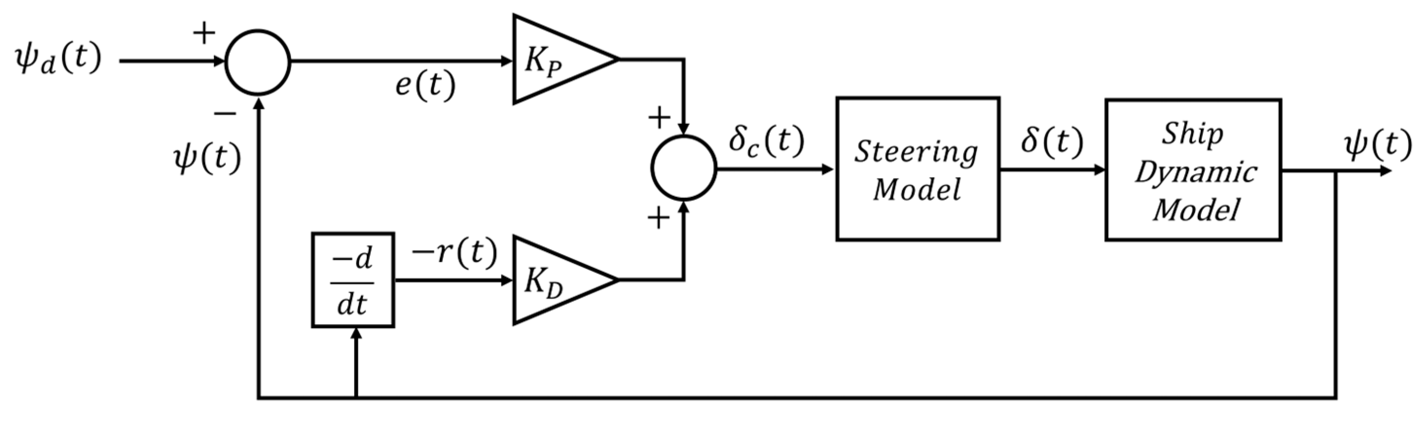
3.3. Heading Controller Design

The automatic steering system of the vessel must be adaptive to shallow water effects, changing environmental conditions, and must have precise and rapid course-changing capabilities while preventing overshoot during large angle turns [44]. Various control methods, such as PID control, sliding mode control, optimal control, fuzzy control, and neural network-based control, are commonly used for heading control of ships [45,46,47,48,49,50]. However, for large vessels like the one considered in this study, the motion characteristics are slow, and the inertia is high, making complex nonlinear controllers unnecessary. A simpler control method, such as the PD controller, can provide sufficient performance [38,51,52,53]. Therefore, in this study, a heading controller was designed and implemented using a PD controller, as shown in Figure 5.

Here, $\psi \left(t\right)$ represents the current heading angle, ${\psi }_d\left(t\right)$ represents the desired heading angle, $K_P$ is the proportional gain, $K_D$ is the derivative gain, $e\left(t\right)$ is the heading angle error defined as ${\psi }_d\left(t\right)-\psi \left(t\right)$, $r\left(t\right)$ is the yaw rate, ${\delta }_c\left(t\right)$ is the commanded rudder angle, and ${\delta }_c\left(t\right)$ represents the actual rudder angle. The PD control equation used to compute the commanded rudder angle is expressed as follows [54]:

$${\delta }_c\left(t\right)=K_{P}e\left(t\right)-K_D{\displaystyle \frac{d\psi \left(t\right)}{dt}}$$

(34)

The computed rudder angle is then input into the ship’s steering model, adjusting the actual rudder angle. The maximum rudder angle is limited to ±35°, and the rudder rate of the model ship KVLCC2 is set to 2.32°/s. Once the rudder angle is adjusted, the ship’s maneuvering motion model calculates the new heading angle accordingly.

The PD controller parameters were tuned using the Ziegler–Nichols method of ultimate sensitivity [55]. In this method, a feedback loop is constructed with only proportional action, and the proportional gain is gradually increased from zero until the output shows sustained oscillations. The proportional gain at this point is called the ultimate gain ($K_u$), and the period of oscillation is called the ultimate period ($T_u$). The ultimate gain and period are then used to determine the initial controller parameters, which are fine-tuned to achieve the desired response [56].

In this study, sustained oscillations were observed when the proportional gain was 18.1, as shown in Figure 6a, with a period of 121 s. Based on the $K_u$ and $T_u$, the initial controller parameters were calculated. After a fine-tuning process, $K_P$ and $K_D$ were set to 8.7 and 173.2, respectively. Using these parameters, a heading controller incorporating the PD controller was constructed, and a step function with a magnitude of 30 was applied as input to measure the step response. Figure 6b shows the step response of KVLCC2.

The rise time ($t_r$) is the time taken for the output to reach from 10% to 90% of the final value, and the settling time ($t_s$) is the time taken for the output to remain within 2% of the final value. The maximum overshoot ($M_p$) is the difference between the peak value and the steady-state value, while the peak time ($t_p$) is the time taken for the output to reach the maximum overshoot. The steady-state error ($e_{ss}$) refers to the difference between the desired output and the actual output in the steady state. The $t_r$ was 58 s, the $t_s$ was 189 s, the $t_p$ was 132 s, the $M_p$ was 1.5 degrees, and the $e_{ss}$ was 0.0022 degrees. These results show that the control parameters of KVLCC2 were appropriately set, as the response time was reasonable with minimal overshoot and the steady-state error was almost negligible.

4. Model Validation and Simulation Results

In this section, we validate the effectiveness of the proposed path-following method for the KVLCC2 vessel. The vessel’s motion model was evaluated using turning circle tests and zigzag tests to assess its maneuverability and response characteristics. Additionally, path-following simulation tests were conducted using the proposed method and the three existing LOS guidance methods. These simulations highlight the advantages of the proposed method, particularly in reducing XTE, minimizing overshoot, and improving overall path-following accuracy during significant course changes.

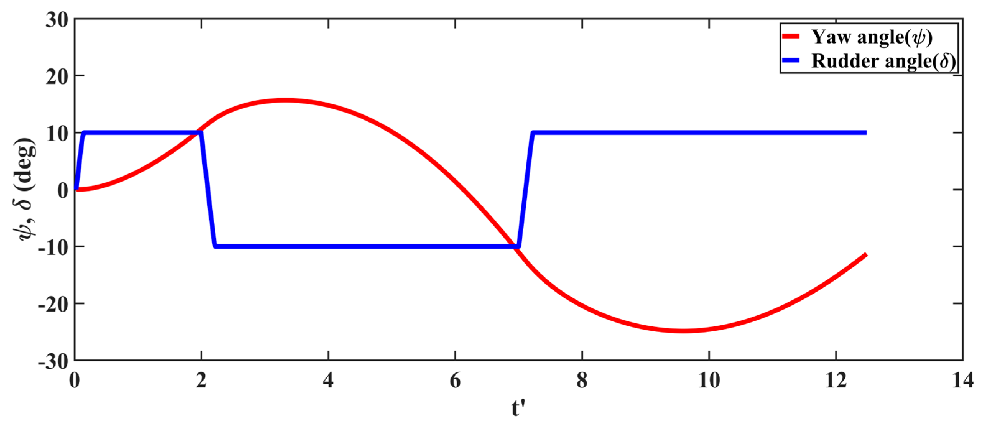
4.1. Validation of KVLCC2 Maneuvering Model

Two maneuvering performance tests were conducted to evaluate the reliability and accuracy of the KVLCC2 maneuvering motion simulator developed in this study. These tests are essential for confirming the simulator’s ability to represent accurately the vessel’s real-world maneuvering characteristics. The results were compared with free-running model test results for KVLCC2 and findings from other studies on its maneuvering performance.

The first test is the turning circle test, where the vessel moves straight at a constant speed before performing a turn by applying a rudder angle of 35° to either port or starboard, forming a turning circle. Key metrics such as the advance, transfer, and tactical diameter are measured to evaluate the vessel’s turning performance and responsiveness [57]. Figure 7 shows the graph of the 35° turning circle test results for KVLCC2, and

Table 3. Comparison of turning maneuver indices of KVLCC2.

		MARIN FR	MANSIM	Yasukawa & Yoshimura	Present Code
+35°	$\mathrm{Ad}./L_{pp}$	3.25	3.10	3.62	3.24
	$\mathrm{Tr}./L_{pp}$	1.36	1.35	1.58	1.37
	$\mathrm{TD}/L_{pp}$	3.34	3.16	3.71	3.18
−35°	$\mathrm{Ad}./L_{pp}$	3.11	3.10	3.56	3.09
	$\mathrm{Tr}./L_{pp}$	−1.22	−1.23	−1.51	−1.24
	$\mathrm{TD}/L_{pp}$	−3.08	−2.90	−3.59	−2.89

provides a comparison of the turning test indices between MARIN FR, MANSIM, Yasukawa and Yoshimura, and this study [35,36,37].

In Figure 7, the axes $x/L$ and $y/L$ represent the dimensionless $x$- and $y$-coordinates, respectively, as both have been normalized by dividing by the length. The turning test results from this study show some differences compared to the results of Yasukawa and Yoshimura. However, the results are generally in good agreement with those from MARIN FR and MANSIM. Specifically, the advance distance matches well with the MARIN FR results, while the transfer distance aligns more closely with the results from MANSIM. Overall, the turning characteristics of KVLCC2 are well-represented.

The second test is the zigzag test, which measures the vessel’s responsiveness by alternately applying a rudder angle to port and starboard to deviate from the original course. The overshoot angles (OAs) are measured, helping to evaluate the vessel’s response characteristics and its ability to return to the course [57]. Figure 8 shows the graph of the 10°/10° zigzag test results for KVLCC2, and

Table 4. Comparison of overshoot angles in zigzag test of KVLCC2.

		MARIN FR	MANSIM	Yasukawa & Yoshimura	Present Code
+10°	1st OA	8.2	5.3	5.8	5.7
	2nd OA	21.9	14.1	20.5	14.9
−10°	1st OA	9.5	7.5	8.8	8.2
	2nd OA	15	9.4	12.6	9.6
+20°	1st OA	13.7	11.1	11.8	11.7
	2nd OA	14.9	15.5	19.7	15.6
−20°	1st OA	15.1	14.2	16.1	14.7
	2nd OA	13.3	11.8	14.6	11.9

provides the OAs from the 10°/10° and 20°/20° zigzag tests, showing results from MARIN FR, MANSIM, Yasukawa and Yoshimura, and this study [35,36,37].

In Figure 8, the horizontal axis means non-dimensionalized time defined as $t’\equiv t{U}_0/L_{pp}$. The zigzag test results from this study show some differences compared to the MARIN FR results, but are generally in good agreement with the results from MANSIM and Yasukawa & Yoshimura. Particularly, the OAs from both the 10°/10° and 20°/20° zigzag tests align closely with the MANSIM results. Since the results of the two maneuvering tests conducted using the simulator developed in this study are within acceptable ranges compared to other studies, the reliability of the simulator is confirmed.

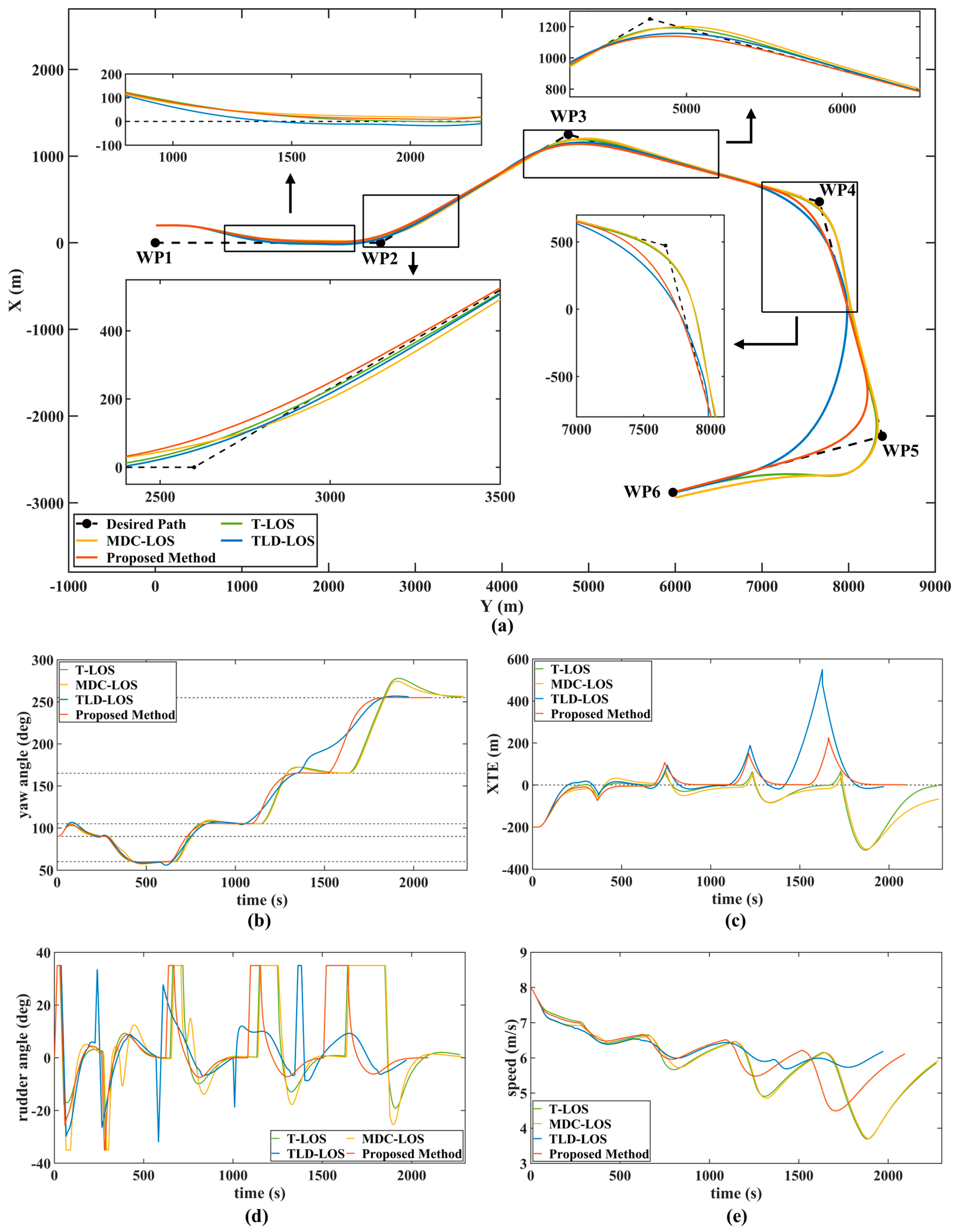
4.2. Path Following Simulation Results

To verify the effectiveness of the proposed path-following method, a simulation test was conducted, and the results were compared with those of the traditional LOS guidance law, LOS guidance using the minimum dynamic circle, and the time-varying lookahead distance guidance law. The primary goal was to evaluate improvements in XTE, course change efficiency, and overall path-following accuracy. Six waypoints were set for the path-following simulation.

Table 5. Waypoint list for path-following simulation test.

	X (m)	Y (m)	Course (°)	Distance (m)	Course Change Angle (°)	${\mathit{R}}_{\mathit{k}}$ (m)
Waypoint 1	0	0
			090	2600
Waypoint 2	0	2600			−30	669
			060	2500
Waypoint 3	1250	4765			45	781
			105	3000
Waypoint 4	473	7663			60	853
			165	2800
Waypoint 5	−2232	8388			90	1038
			255	2500
Waypoint 6	−2879	5973

shows the six waypoints, the angles and distances between the waypoints, and the distance of the new course for each waypoint. The circle of acceptance was calculated using the turning circle test results and Equation (31), allowing for dynamic adjustments based on the course change angle.

The vessel’s initial position was set at (200, 0), with an initial course of 090° and an initial speed of 7.97 m/s. The initial position was intentionally offset from waypoint 1 to verify if the vessel could properly converge to the original course between waypoint 1 and waypoint 2. After converging to the original course, the vessel changed its heading following a sequence of port 30°, starboard 45°, starboard 60°, and starboard 90° as it navigated along the predefined path.

The parameter $R_k$ for the traditional LOS guidance law and LOS guidance using the minimum dynamic circle was set to twice the ship’s length, as is generally recommended, while $R_o$ was set to 2.5 times the ship’s length for the traditional guidance to ensure the condition $R_o\ge R_k$ was satisfied. For the time-varying lookahead distance guidance law, the parameters were set as ${\Delta }_{max}=640$, ${\Delta }_{min}=800,$ and $\gamma =0.01$, based on numerous simulation experiments, with $R_k$ dynamically adjusted according to Equation (25). On the other hand, the proposed method dynamically calculated both $R_k$ and $R_o$ in real-time, using Equations (31) and (32), respectively.

Figure 9 shows the path-following simulation results using the proposed method, indicated by the red line, the traditional LOS guidance law (T-LOS), represented by the green line, the LOS guidance using minimum dynamic circle (MDC-LOS), shown by the yellow line, and the time-varying lookahead distance guidance law (TLD-LOS), represented by the blue line.

In the early stage of the simulation, the vessel converged to the original course in the order of TLD-LOS, T-LOS, the proposed method, and MDC-LOS. TLD-LOS and T-LOS resulted in overshoots of approximately 17.8 m and 2.0 m beyond the original course, respectively, while the proposed method and MDC-LOS showed no overshoot but exhibited XTEs of about 8.9 m and 16.5 m, respectively. This is due to the XTL for the proposed method being set to 80 m, which is 0.25 times the ship’s length. This slowed the convergence process when the XTE was within that range. As a result, the vessel initiated a course change before fully converging to the original course, leading to a relatively larger XTE.

The differences between the four methods become more pronounced during course changes, especially when the course change angle is larger. At Waypoint 2, where the course change angle was relatively small at 30°, the differences between the methods were minimal. TLD-LOS had the smallest XTE at 46.0 m, followed by T-LOS at 54.2 m, MDC-LOS at 61.6 m, and the proposed method at 72.9 m. In terms of maximum overshoot, MDC-LOS had the largest at 32.0 m, followed by TLD-LOS at 15.8 m, T-LOS at 8.4 m, while the proposed method showed no overshoot.

At waypoints 3, 4, and 5, where the course change angles were 45°, 60°, and 90°, the differences became more noticeable. T-LOS and MDC-LOS had significantly larger overshoot with increasing course change angles, likely due to $R_k$ being fixed at $2L_{pp}$, which limited the distance available for course changes. Additionally, with $R_o$ fixed at $2.5L_{pp}$, the traditional LOS method struggled to generate an effective LOS angle to follow the new course.

TLD-LOS maintained a consistent overshoot regardless of the course change angle, but its XTE increased significantly as the angle increased. This is likely because, unlike T-LOS and MDC-LOS, TLD-LOS dynamically adjusted $R_k$ based on the course change angle, allowing it to start course changes earlier. However, by not considering the ship’s maneuvering characteristics, TLD-LOS initiated the course change too early, resulting in excessive XTE beyond the appropriate waypoint switch point.

In contrast, the proposed method dynamically adjusted $R_k$ and $R_o$ in real-time according to the course change angle and the vessel’s heading angle, minimizing overshoot regardless of the course change angle. However, larger course change angles led to larger XTEs due to the vessel’s steering characteristics, as it follows a curved trajectory instead of a straight path. Despite this, the impact on overall performance was minimal.

In summary, the T-LOS required the rudder to be used at larger angles for longer periods due to the fixed $R_k$ and $R_o$, leading to significant speed reduction. The total time to follow the entire path was 2270 s, and the mean absolute cross-track error (MAE) was 58.33 m. Additionally, T-LOS exhibited increasing overshoot as the course change angles grew larger, with a maximum overshoot of 309.6 m at a 90° course change.

The MDC-LOS, while similar to T-LOS in some aspects, showed a slightly better XTE profile at certain course change angles, such as 60°, but had substantial overshoot as well, reaching 305.0 m at 90°. It completed the path in 2281 s with an MAE of 70.79 m, which was higher than T-LOS.

The TLD-LOS maintained a consistent overshoot across different course change angles, indicating better control over sudden directional changes. However, it struggled with significantly higher XTE at larger course change angles, with the XTE reaching 548.8 m at a 90° turn. Despite finishing the path in the shortest time of 1972 s, its MAE of 69.31 m demonstrated less accurate path-following performance compared to the proposed method.

In contrast, the proposed method dynamically adjusted both $R_k$ and $R_o$ in real-time, based on the course change angle, XTE and the ship’s yaw angle, allowing for a more balanced approach. It minimized overshoot, showing almost no overshoot at all course change angles, while maintaining a reasonable XTE even at larger course changes. The total time to complete the path was 2098 s, and the MAE was the lowest among all methods at 34.38 m, highlighting its superior accuracy in path following.

A limitation of the proposed method is that it does not consider environmental factors such as wind, waves, or currents. However, despite this, the method still demonstrated strong overall performance in path following. Incorporating such factors in future research could further enhance its robustness and applicability in real-world scenarios.

Table 6. Comparison of path-following performance.

	Max. XTE (m)				Max. Overshoot (m)				Time (s)	MAE (m)
	30°	45°	60°	90°	30°	45°	60°	90°
T-LOS	54.2	61.3	84.6	309.6	8.4	30.4	84.6	309.6	2270	58.33
MDC-LOS	61.6	67.0	83.1	305.0	32.0	50.6	83.1	305.0	2281	70.79
TLD-LOS	46.0	94.4	188.5	548.8	15.8	19.0	18.9	16.4	1972	69.31
Proposed method	72.9	103.2	146.0	221.4	-	0.2	0.5	-	2098	34.38

compares the performance metrics of T-LOS, MDC-LOS, TLD-LOS, and the proposed method including the XTE, maximum overshoot distance, time required to follow the desired path, and the MAE. The proposed method demonstrated the best overall balance of rapid convergence to the original course and smooth course changes, making it the most effective for path following across various scenarios.

5. Conclusions

In this study, we proposed a new path-following method based on the distance of new course and XTE to improve the path-following performance of autonomous vessels. The proposed method was specifically designed to account for the maneuvering characteristics of the vessel, offering the advantage of setting the parameters required for path following using only the advance and transfer distances obtained from the turning circle test.

Simulation results demonstrated that the proposed method outperformed T-LOS, MDC-LOS, and TLD-LOS in several key metrics. The total time required to follow the entire path was reduced by approximately 8% compared to T-LOS and MDC-LOS. The MAE was significantly lower, with the proposed method achieving 34.38 m, compared to 58.33 m for T-LOS, 70.79 m for MDC-LOS, and 69.31 m for TLD-LOS. Additionally, while TLD-LOS maintained a consistent overshoot across course changes, the proposed method eliminated overshoot in all scenarios. In terms of XTE, the proposed method showed more balanced performance across different course change angles, particularly when compared to TLD-LOS, which exhibited excessive XTE at larger course change angles.

These findings suggest that the proposed method allows autonomous vessels to follow routes reliably and efficiently even under various path conditions. However, one limitation of this study is that it did not account for external environmental factors such as waves, wind, and currents, which are critical in real maritime environments. Future research should address this limitation by integrating the proposed method with other LOS algorithms capable of handling environmental disturbances, as well as testing the method in real-world scenarios involving more complex vessel dynamics and environmental conditions. Additionally, combining the proposed method with adaptive control algorithms could improve its robustness, ensuring better performance under challenging conditions such as strong winds or currents. These enhancements will strengthen the method’s applicability for autonomous vessels in practical maritime operations.

References

1. Barrera, C.; Padron, I.; Luis, F.S.; Llinas, O.; Marichal, G.N. Trends and Challenges in Unmanned Surface Vehicles (USV): From Survey to Shipping. TransNav Int. J. Mar. Navig. Saf. Sea Transp. 2021, 15, 135–142. [Google Scholar] [CrossRef]
2. Munim, Z.H.; Haralambides, H. Advances in maritime autonomous surface ships (MASS) in merchant shipping. Marit. Econ. Logist. 2022, 24, 181–188. [Google Scholar] [CrossRef]
3. Lynch, K.M.; Banks, V.A.; Roberts, A.P.; Radcliffe, S.; Plant, K.L. What factors may influence decision-making in the operation of Maritime autonomous surface ships? A systematic review. Theor. Issues Ergon. Sci. 2024, 25, 98–142. [Google Scholar] [CrossRef]
4. Qiao, Y.; Yin, J.; Wang, W.; Duarte, F.; Yang, J.; Ratti, C. Survey of Deep Learning for Autonomous Surface Vehicles in Marine Environments. IEEE Trans. Intell. Transp. Syst. 2023, 24, 3678–3701. [Google Scholar] [CrossRef]
5. Statheros, T.; Howells, G.; Maier, K.M. Autonomous ship collision avoidance navigation concepts, technologies and techniques. J. Navig. 2008, 61, 129–142. [Google Scholar] [CrossRef]
6. Wang, J.; Xiao, Y.; Li, T.; Chen, C.L.P. A Survey of Technologies for Unmanned Merchant Ships. IEEE Access 2020, 8, 224461. [Google Scholar] [CrossRef]
7. Öztürk, Ü.; Akdağ, M.; Ayabakan, T. A review of path planning algorithms in maritime autonomous surface ships: Navigation safety perspective. Ocean Eng. 2022, 251, 111010. [Google Scholar] [CrossRef]
8. Zhang, X.; Wang, C.; Jiang, L.; An, L.; Yang, R. Collision-avoidance navigation systems for Maritime Autonomous Surface Ships: A state of the art survey. Ocean Eng. 2021, 235, 109380. [Google Scholar] [CrossRef]
9. Akdağ, M.; Solnør, P.; Johansen, T.A. Collaborative collision avoidance for maritime autonomous surface ships: A review. Ocean Eng. 2022, 250, 110920. [Google Scholar] [CrossRef]
10. Issa, M.; Llinca, A.; Ibrahim, H.; Rizk, P. Maritime autonomous surface ships: Problems and challenges facing the regulatory process. Sustainability 2022, 14, 15630. [Google Scholar] [CrossRef]
11. Liu, C.; Chu, X.; Wu, W.; Li, S.; He, Z.; Zheng, M.; Zhou, H.; Li, Z. Human–machine cooperation research for navigation of maritime autonomous surface ships: A review and consideration. Ocean Eng. 2022, 246, 110555. [Google Scholar] [CrossRef]
12. Budak, G.; Beji, S. Controlled course-keeping simulations of a ship under external disturbances. Ocean Eng. 2020, 218, 108126. [Google Scholar] [CrossRef]
13. Healey, A.J.; Lienard, D. Multivariable sliding mode control for autonomous diving and steering of unmanned underwater vehicles. IEEE J. Ocean. Eng. 1993, 18, 327–339. [Google Scholar] [CrossRef]
14. Breivik, M. Nonlinear Maneuvering Control of Underactuated Ships. Master’s Thesis, Norwegian University of Science and Technology, Trondheim, Norway, 2003. [Google Scholar]
15. Lekkas, A.M.; Fossen, T.I. Line-of-sight guidance for path following of marine vehicles. In Advanced in Marine Robotics; Gal, O., Ed.; Academic: San Francisco, CA, USA, 2013; pp. 63–92. [Google Scholar]
16. Gu, N.; Wang, D.; Peng, Z.; Wang, J.; Han, Q. Advances in Line-of-Sight Guidance for Path Following of Autonomous Marine Vehicles: An Overview. IEEE Trans. Syst. Man Cybern. Syst. 2023, 53, 12–28. [Google Scholar] [CrossRef]
17. Børhaug, E.; Pavlov, A.; Pettersen, K.Y. Integral LOS control for path following of underactuated marine surface vessels in the presence of constant ocean currents. In Proceedings of the 2008 47th IEEE Conference on Decision and Control, Cancun, Mexico, 9–11 December 2008; pp. 4984–4991. [Google Scholar] [CrossRef]
18. Lekkas, A.M.; Fossen, T.I. Integral LOS Path Following for Curved Paths Based on a Monotone Cubic Hermite Spline Parametrization. IEEE Trans. Control Syst. Technol. 2014, 22, 2287–2301. [Google Scholar] [CrossRef]
19. Wan, L.; Su, Y.; Zhang, H.; Shi, B.; Abouomar, M.S. An improved integral light-of-sight guidance law for path following of unmanned surface vehicles. Ocean Eng. 2020, 205, 107302. [Google Scholar] [CrossRef]
20. Han, B.; Duan, Z.; Peng, Z.; Chen, Y. A Ship Path Tracking Control Method Using a Fuzzy Control Integrated Line-of-Sight Guidance Law. J. Mar. Sci. Eng. 2024, 12, 586. [Google Scholar] [CrossRef]
21. Fossen, T.I.; Pettersen, K.Y.; Galeazzi, R. Line-of-Sight Path Following for Dubins Paths With Adaptive Sideslip Compensation of Drift Forces. IEEE Trans. Control Syst. Technol. 2015, 23, 820–827. [Google Scholar] [CrossRef]
22. Liu, L.; Wang, D.; Peng, Z.; Wang, H. Predictor-based LOS guidance law for path following of underactuated marine surface vehicles with sideslip compensation. Ocean Eng. 2016, 124, 340–348. [Google Scholar] [CrossRef]
23. Liu, L.; Wang, D.; Peng, Z. ESO-Based Line-of-Sight Guidance Law for Path Following of Underactuated Marine Surface Vehicles With Exact Sideslip Compensation. IEEE J. Ocean. Eng. 2017, 42, 477–487. [Google Scholar] [CrossRef]
24. Nie, J.; Lin, X. FAILOS guidance law based adaptive fuzzy finite-time path following control for underactuated MSV. Ocean Eng. 2020, 195, 106726. [Google Scholar] [CrossRef]
25. Fossen, T.I.; Pettersen, K.Y. On uniform semiglobal exponential stability (USGES) of proportional line-of-sight guidance laws. Automatica 2014, 50, 2912–2917. [Google Scholar] [CrossRef]
26. Rout, R.; Cui, R.; Han, Z. Modified line-of-sight guidance law with adaptive neural network control of underactuated marine vehicles with state and input constraints. IEEE Trans. Control Syst. Technol. 2020, 28, 1902–1914. [Google Scholar] [CrossRef]
27. Qiu, B.; Wang, G.; Fan, Y. Predictor LOS-based trajectory linearization control for path following of underactuated unmanned surface vehicle with input saturation. Ocean Eng. 2020, 214, 107874. [Google Scholar] [CrossRef]
28. Fossen, T.I. Line-of-sight path-following control utilizing an extended Kalman filter for estimation of speed and course over ground from GNSS positions. J. Mar. Sci. Eng. 2022, 27, 806–813. [Google Scholar] [CrossRef]
29. Lv, C.; Liu, L.; Wang, D.; Peng, Z.; Li, Y.; Li, T. Human-machine Shared Line-of-Sight Path Following Control of Intelligent Surface Vehicles. IEEE Trans. Veh. Technol, 2024; early access. [Google Scholar] [CrossRef]
30. Fossen, T.I.; Breivik, M.; Skjetne, R. Line-of-sight path following of underactuated marine craft. In Proceedings of the 2003 6th IFAC Conference on Manoeuvring and Control of Marine Craft, Girona, Spain, 17–19 September 2003; Volume 36, pp. 211–216. [Google Scholar] [CrossRef]
31. Moreira, L.; Fossen, T.I.; Guedes Soares, C. Path following control system for a tanker ship model. Ocean Eng. 2007, 34, 2074–2085. [Google Scholar] [CrossRef]
32. Lekkas, A.M.; Fossen, T.I. A time-varying lookahead distance guidance law for path following. In Proceedings of the 2012 9th IFAC Conference on Manoeuvring and Control of Marine Craft, Arenzano, Italy, 19–21 September 2012; Volume 45, pp. 398–403. [Google Scholar] [CrossRef]
33. Su, Z.; Zhang, X. Nonlinear Feedback-Based Path Following Control for Underactuated Ships via an Improved Compound Line-of-Sight Guidance. IEEE Access 2021, 9, 81535–81545. [Google Scholar] [CrossRef]
34. Fossen, T.I. Guidance and Control of Ocean Vehicle; John Wiley & Sons Ltd.: Chichester, UK, 1994. [Google Scholar]
35. Yasukawa, H.; Yoshimura, Y. Introduction of MMG standard method for ship maneuvering predictions. J. Mar. Sci. Technol. 2014, 20, 37–52. [Google Scholar] [CrossRef]
36. SIMMAN. Part C: Captive and free model test data. In Proceedings of the Workshop on Verification and Validation of Ship Manoeuvring Simulation Methods (SIMMAN), Copenhagen, Denmark, 14–16 April 2008; SIMMAN: Copenhagen, Denmark, 2008.
37. Sukas, O.F.; Kinaci, O.K.; Bal, S. Theoretical background and application of MANSIM for ship maneuvering simulations. Ocean Eng. 2019, 192, 106239. [Google Scholar] [CrossRef]
38. Paramesh, S.; Rajendran, S. A unified seakeeping and manoeuvring model with a PID controller for path following of a KVLCC2 tanker in regular waves. Appl. Ocean Res. 2021, 116, 102860. [Google Scholar] [CrossRef]
39. Adams, J.; Dubey, A.C.; Rajendran, S. A Model Predictive based Controller (MPC) for the Path Following of a KVLCC2 Tanker in waves. In Proceedings of the IEEE OCEANS Conferences 2022, Chennai, India, 21–24 February 2022. [Google Scholar] [CrossRef]
40. Kim, D.J.; Choi, H.; Yun, K.; Yeo, D.J.; Kim, Y.G. Experimental study on turning characteristics of KVLCC2 tanker in long-crested irregular waves. Ocean Eng. 2022, 244, 110362. [Google Scholar] [CrossRef]
41. Fossen, T.I. Marine Control Systems C Guidance. Navigation, and Control of Ships, Rigs and Underwater Vehicles; Marine Cybern.: Trondheim, Norway, 2002. [Google Scholar]
42. Papoulias, F.A. Bifurcation analysis of line of sight vehicle guidance using sliding modes. Int. J. Bifurc. Chaos 1991, 1, 849–865. [Google Scholar] [CrossRef]
43. Kamis, A.S.; Ahmad Fuad, A.F.; Ashaari, A.; Mohd Noor, C.W. Development of WOP mathematical model for efficient course alteration: LNG tanker manoeuvring analysis and Mann-Whitney U test. Ocean Eng. 2021, 239, 109768. [Google Scholar] [CrossRef]
44. Fossen, T.I. Recent Developments in Ship Control Systems Design. World Superyacht Review; Sterling Publication Limited: London, UK, 1999. [Google Scholar]
45. Zhang, R.; Chen, Y.; Sun, Z.; Sun, F.; Xu, H. Path control of a surface ship in restricted waters using sliding mode. IEEE Trans. Control Syst. Technol. 2000, 8, 722–732. [Google Scholar] [CrossRef] [PubMed]
46. Perera, L.P.; Soares, C.G. Pre-filtered sliding mode control for nonlinear ship steering associated with disturbances. Ocean Eng. 2012, 51, 49–62. [Google Scholar] [CrossRef]
47. Layne, J.R.; Passino, K.M. Fuzzy model reference learning control for cargo ship steering. IEEE Control Syst. 1993, 13, 23–34. [Google Scholar] [CrossRef]
48. Velagic, J.; Vukic, Z.; Omerdic, E. Adaptive fuzzy ship autopilot for track-keeping. Control Eng. Pract. 2003, 11, 433–443. [Google Scholar] [CrossRef]
49. Zhang, Y.; Hearn, G.E.; Sen, P. A neural network approach to ship track-keeping control. IEEE J. Ocean. Eng. 1996, 21, 513–527. [Google Scholar] [CrossRef]
50. Dai, S.L.; Wang, C.; Luo, F. Identification and learning control of ocean surface ship using neural networks. IEEE Trans. Ind. Inform. 2012, 8, 801–810. [Google Scholar] [CrossRef]
51. Dubey, A.C.; Gajapathy, R.; Rajendran, S. An experimental and numerical investigation on the autopilot design of a KVLCC2 tanker. In Proceedings of the IEEE OCEANS Conferences, San Diego, CA, USA, 20–23 September 2021. [Google Scholar] [CrossRef]
52. Sandeepkumar, R.; Rajendran, S.; Mohan, R.; Pascoal, A. A unified ship manoeuvring model with a nonlinear model predictive controller for path following in regular waves. Ocean Eng. 2022, 243, 110165. [Google Scholar] [CrossRef]
53. Paramesh, S.; Rajendran, S. Numerical investigation of the manoeuvring motions and trajectory tracking of a kvlcc2 tanker using PID controller in regular waves. In Proceedings of the Global Oceans 2020, Biloxi, MS, USA, 5–30 October 2020. [Google Scholar] [CrossRef]
54. Fossen, T.I. Handbook of Marine Craft Hydrodynamics and Motion Control; John Wiley & Sons: Hoboken, NJ, USA, 2011. [Google Scholar]
55. Ziegler, J.G.; Nichols, N.B. Optimum settings for automatic controllers. Trans. ASME 1942, 64, 759–765. [Google Scholar] [CrossRef]
56. McCormack, A.S.; Godfrey, K.R. Rule-based autotuning based on frequency domain identification. IEEE Trans. Control Syst. Technol. 1998, 6, 43–61. [Google Scholar] [CrossRef]
57. International Maritime Organization (IMO). Standards for Ship Manoeuvrability (IMO Resolution MSC.137(76)); IMO: London, UK, 2002. [Google Scholar]
Figure 1. Coordinate systems.
Jmse 12 01831 g001
Figure 2. Traditional LOS guidance law.
Jmse 12 01831 g002
Figure 3. Time-varying lookahead distance guidance law.
Jmse 12 01831 g003
Figure 5. Block diagram of heading controller.
Jmse 12 01831 g005
Figure 6. PD controller parameter tuning: (a) ultimate oscillation; (b) step response.
Jmse 12 01831 g006
Figure 7. Turning test for KVLCC2 ( ± 35 ° ).
Jmse 12 01831 g007
Figure 8. ZigZag test for KVLCC2 ( ± 35 ° ).
Jmse 12 01831 g008
Figure 9. Path following simulation test results: (a) ship’s trajectories following the desired path; (b) yaw angles; (c) cross-track errors; (d) rudder angles; (e) speeds.
Jmse 12 01831 g009