


Investigation into Using CFD for Estimation of Ship Specific Parameters for the SPICE Model for Prediction of Sea Spray Icing: Part 1—The Proposal


Abstract
1. Introduction
2. Methodology
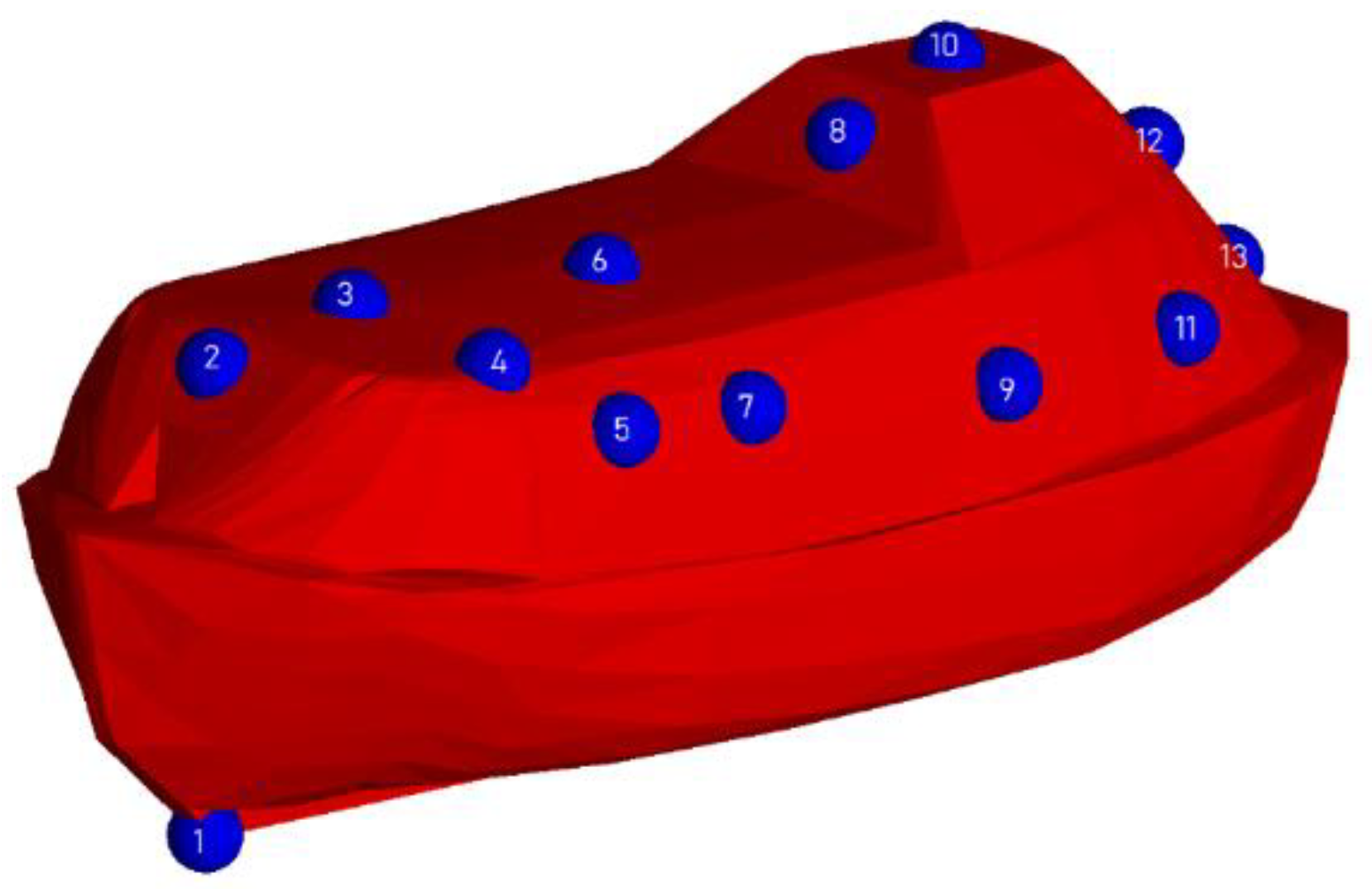
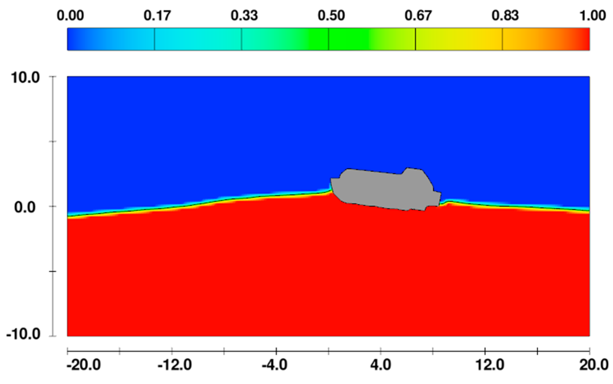
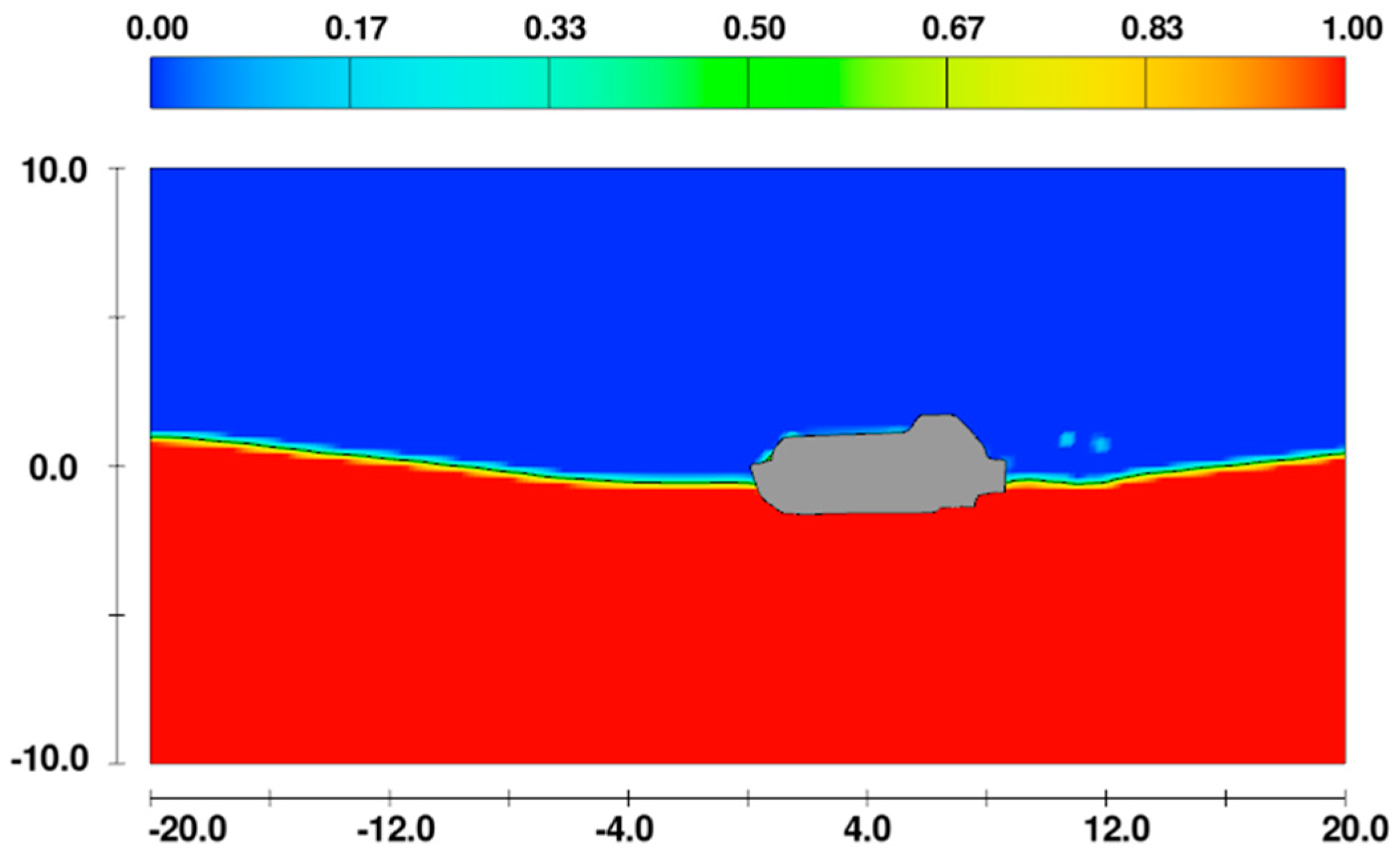
2.1. The Case
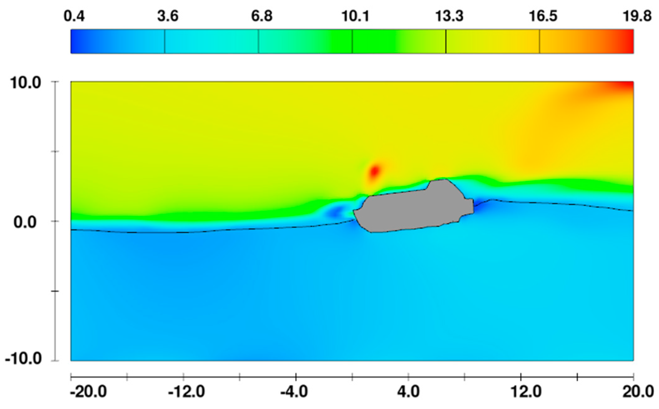
2.2. CFD Simulation Setup
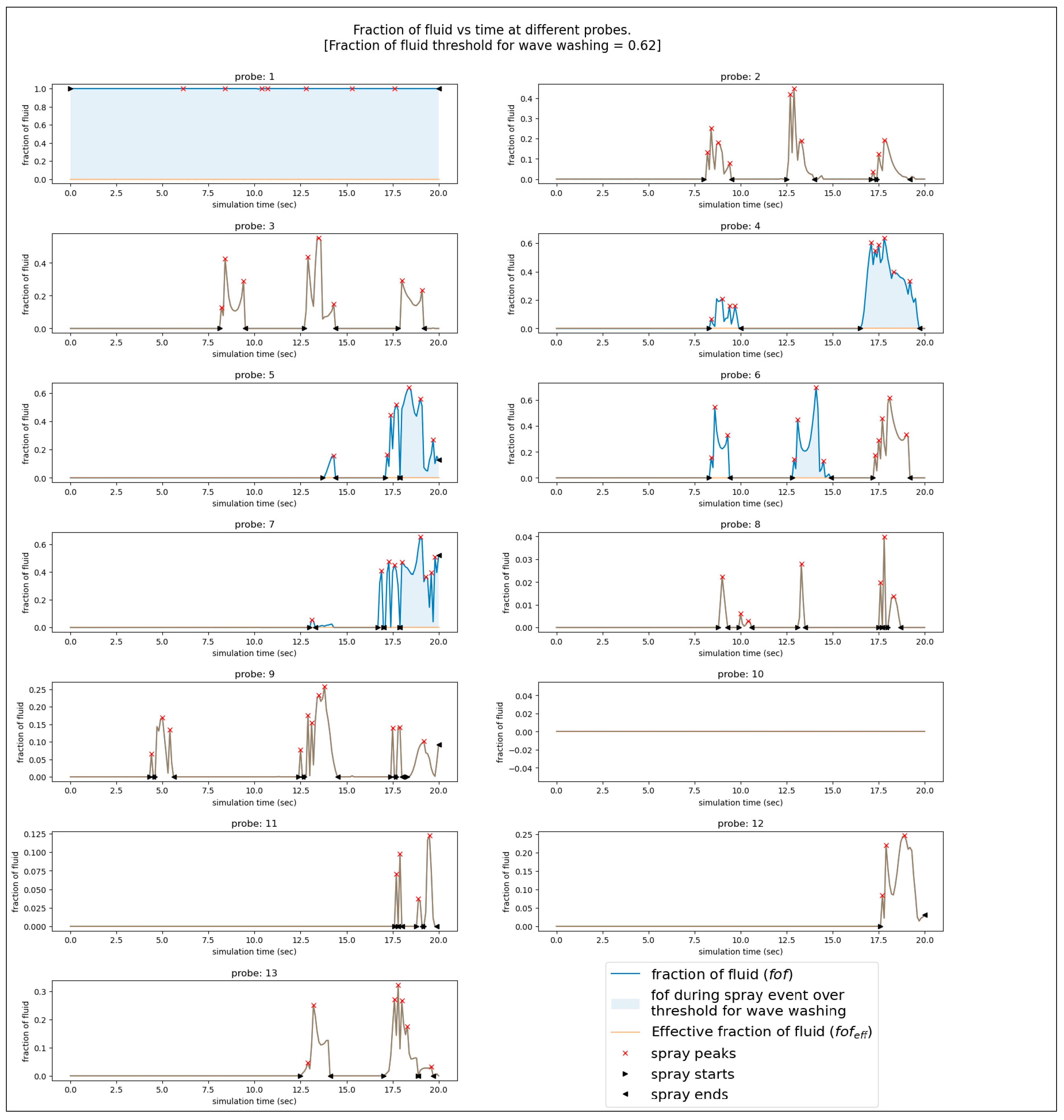
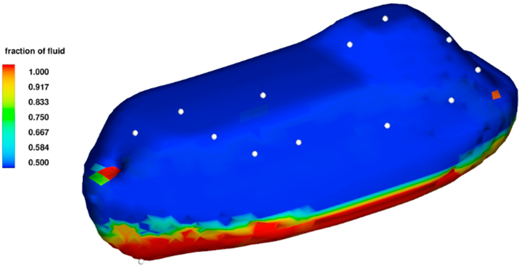
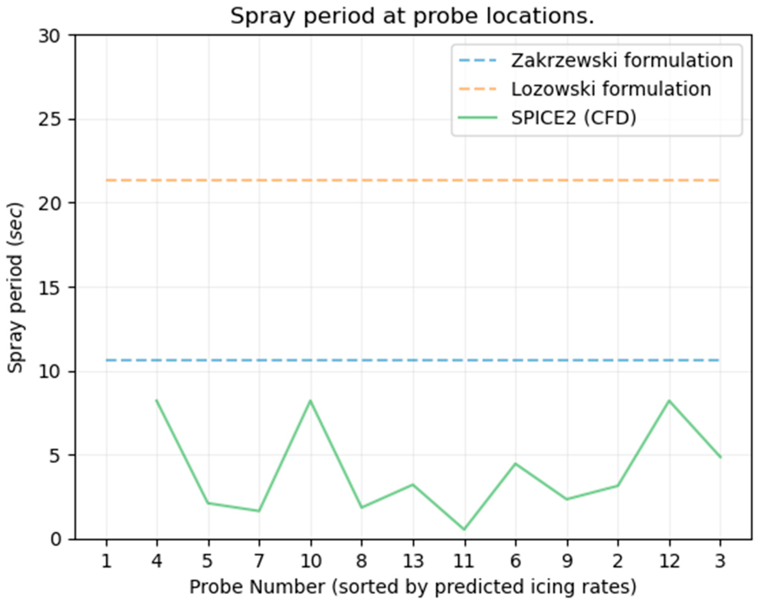
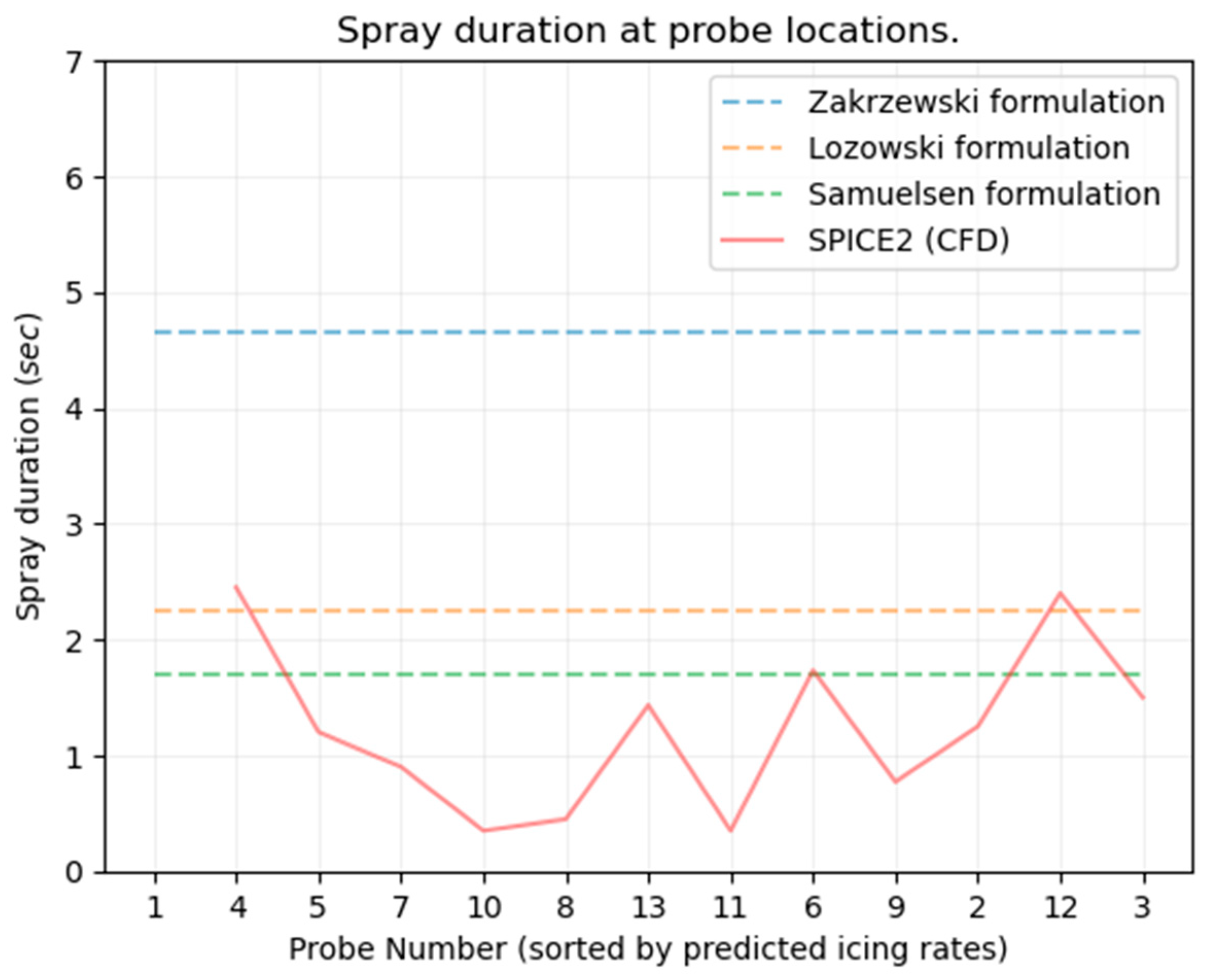
2.3. Post-Processing of CFD Results
2.4. The SPICE Model
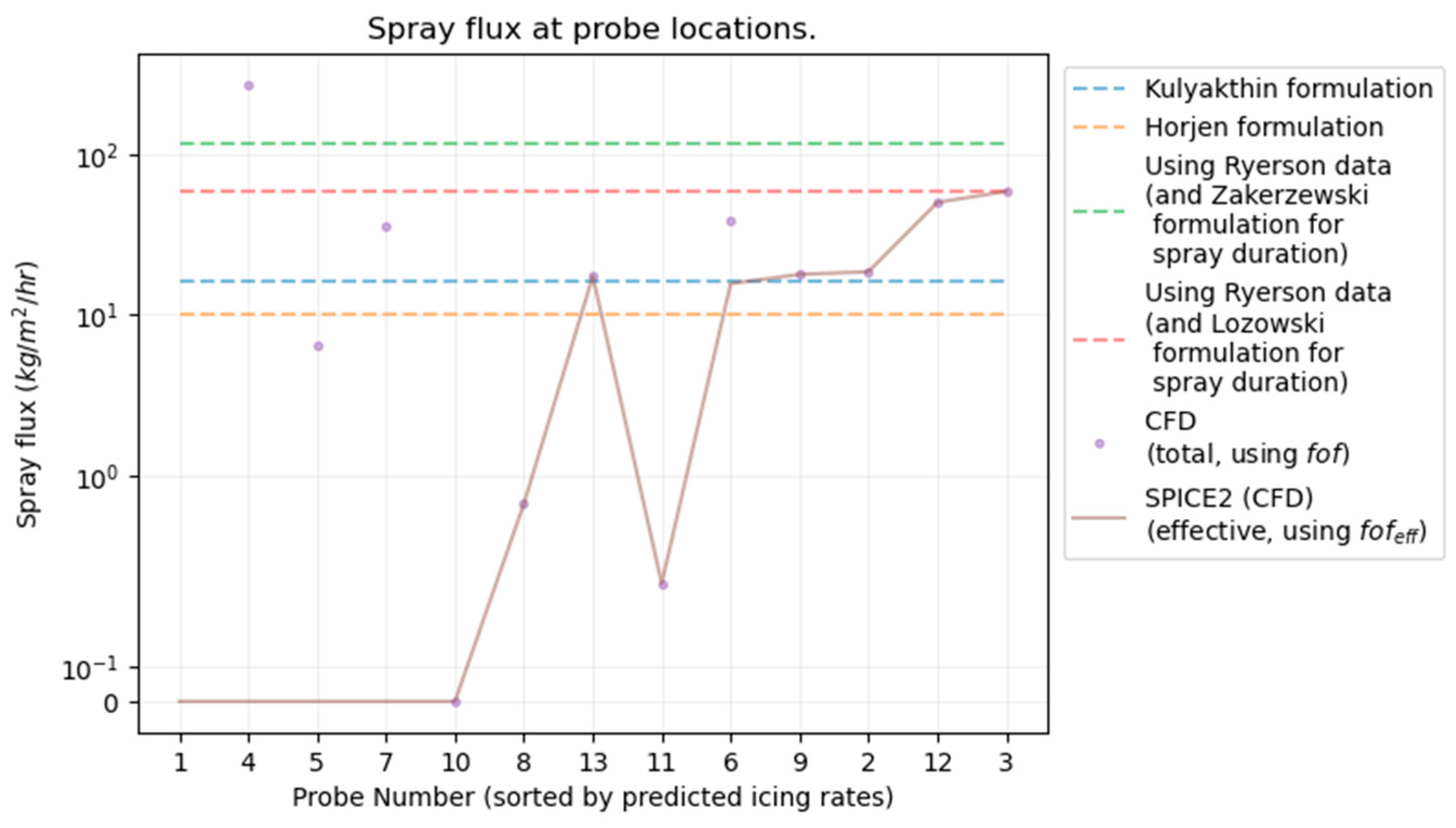
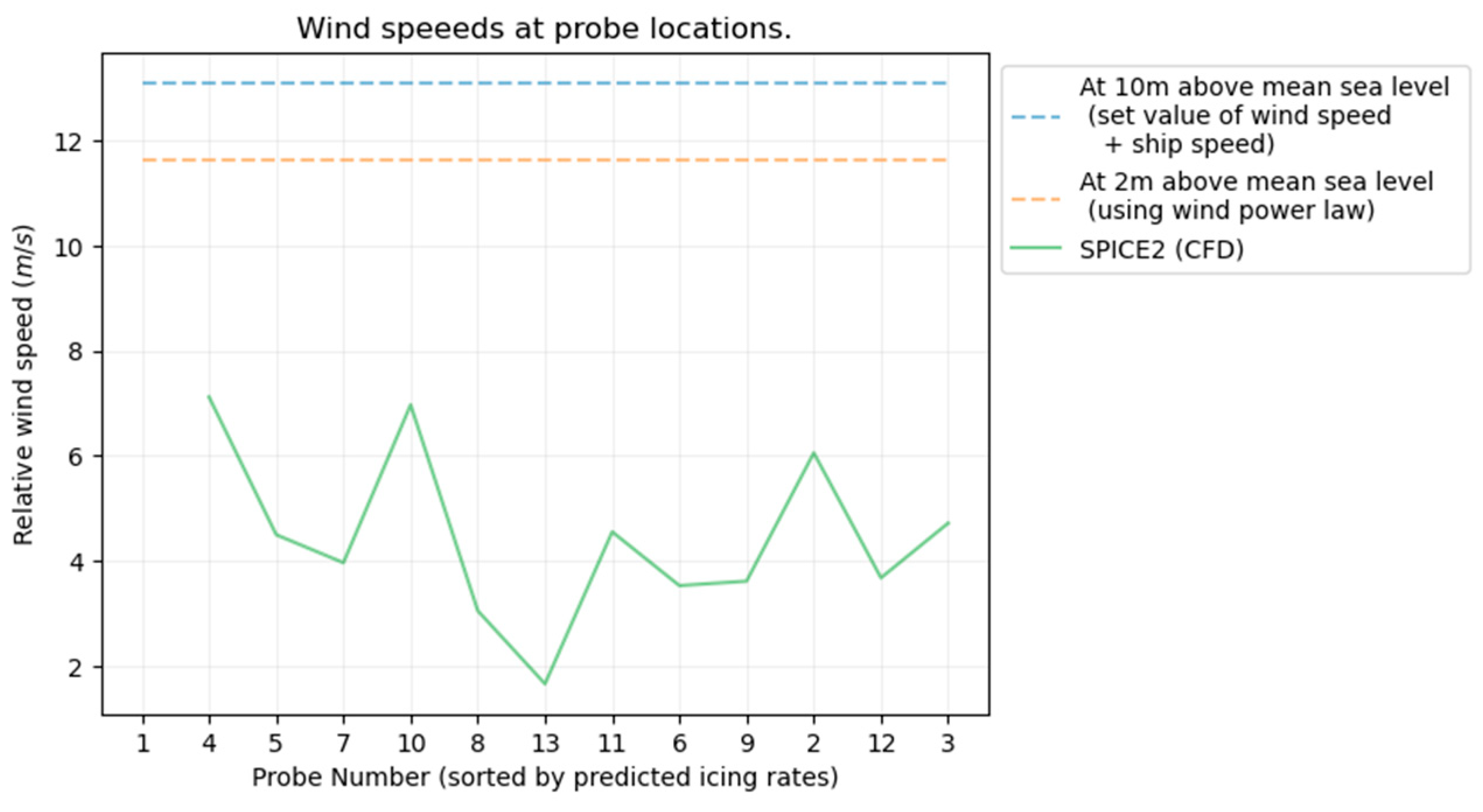
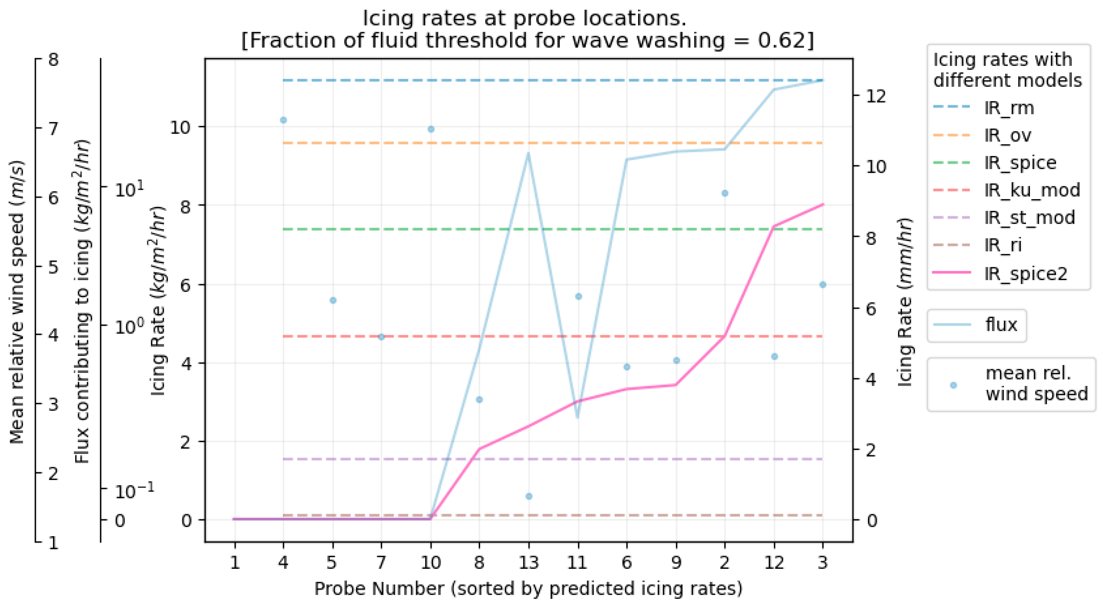
3. Results
Addressing Safety Considerations and Environmental Impact
4. Conclusions and Discussion
Author Contributions
Funding
Institutional Review Board Statement
Informed Consent Statement
Data Availability Statement
Acknowledgments
Conflicts of Interest
Nomenclature
| Symbol | Unit | Description | Comment |
| fof | - | Fraction of fluid in open volume of a cell | |
| fofeff | - | Effective fraction of fluid after considering wave washing | |
| g | m/s2 | Acceleration due to gravity | g = 9.81 m/s2 |
| i | - | ith spray event | |
| N | - | Number of spray events in time tsim | |
| Nhr | - | Number of sprays per hour | |
| Ts | s | Wave period | |
| us | m/s | Ship speed | |
| uz | m/s | Wind speed at a height of z m over the mean sea level | |
| u10 | m/s | Wind speed at a height of 10 m over the mean sea level | |
| t | s | Time | |
| tend | s | End time of spray event | |
| tsim | s | Total simulation time | |
| tstart | s | Start time of spray event | |
| u | m/s | Velocity in x direction | Subscripts: probe, fluid |
| u* | m/s | Friction velocity | |
| v | m/s | Velocity in y direction | Subscripts: probe, fluid |
| vf | m3 | Volume of fluid in a cell | |
| vf_eff | m3 | Effective volume of fluid in a cell | |
| vfin | m3/s | Volume of fluid entering the cell per sec | |
| vfin_eff | m3/s | Effective volume of fluid entering the cell per sec | |
| vf1 | - | Fraction of lifeboat in cell | |
| w | m/s | Velocity in z direction | Subscripts: probe, fluid |
| wsrel | m/s | Relative wind speed | |
| z | m | Height above mean sea level | |
| zwaterSurface | m | Instantaneous height of the water surface at the inlet | |
| z0 | m | Friction coefficient | For wind power law |
| κ | von Kármán constant | κ = 0.41 | |
| λ | m | Wavelength | |
| ρw | kg/m3 | Density of seawater | |
| τdur | sec | Spray duration | |
| τper | s−1 | Spray period | |
| φ | kg/m2/h | Spray flux | |
| ω | m | Length of mesh cell |
References
- Kulyakhtin, A. Numerical Modelling and Experiments on Sea Spray Icing. Ph.D. Thesis, Department of Civil and Transport Engineering, Norwegian University of Science and Technology (NTNU), Trondheim, Norway, 2014. [Google Scholar]
- Lozowski, E.P.; Szilder, K.; Makkonen, L. Computer simulation of marine ice accretion. Philos. Trans. R. Soc. London. Ser. A Math. Phys. Eng. Sci. 2000, 358, 2811–2845. [Google Scholar] [CrossRef]
- Stallabrass. Trawler Icing—A Compilation of Work Done at N. R. C.; Mechanical Engineering Report MD-56, N.R.C. No. 19372; National Research Council: Ottawa, ON, Canada, 1980.
- Zakrzewski, W.P. Splashing a ship with collision-generated spray. Cold Reg. Sci. Technol. 1987, 14, 65–83. [Google Scholar] [CrossRef]
- Kulyakhtin, A.; Shipilova, O.; Libby, B.; Løset, S. Full-scale 3D CFD Simulation of Spray Impingement on a Vessel Produced by Ship-wave Interaction. In Proceedings of the 21st IAHR International Symposium on Ice (2012), Dalian, China, 11–15 June 2012; pp. 1129–1141. [Google Scholar]
- Samuelsen, E.M.; Edvardsen, K.; Graversen, R.G. Modelled and observed sea-spray icing in Arctic-Norwegian waters. Cold Reg. Sci. Technol. 2017, 134, 54–81. [Google Scholar] [CrossRef]
- Deshpande, S. A Machine Learning Model for Prediction of Marine Icing. J. Offshore Mech. Arct. Eng. 2024, 146, 061601. [Google Scholar] [CrossRef]
- ISO 35106; Petroleum and Natural Gas Industries—Arctic Operations—Metocean, Ice, and Seabed Data. International Organization for Standardization: Geneva, Switzerland, 2017.
- Deshpande, S.; Sæterdal, A.; Sundsbø, P.-A. Experiments with Sea Spray Icing: Investigation of Icing Rates. J. Offshore Mech. Arct. Eng. 2024, 146, 011601. [Google Scholar] [CrossRef]
- Kulyakhtin, A.; Tsarau, A. A time-dependent model of marine icing with application of computational fluid dynamics. Cold Reg. Sci. Technol. 2014, 104–105, 33–44. [Google Scholar] [CrossRef]
- Ryerson, C.C. Superstructure spray and ice accretion on a large U.S. Coast Guard cutter. Atmos. Res. 1995, 36, 321–337. [Google Scholar] [CrossRef]
- Deshpande, S.; Sæterdal, A.; Sundsbø, P.-A. Sea Spray Icing: The Physical Process and Review of Prediction Models and Winterization Techniques. J. Offshore Mech. Arct. Eng. 2021, 143, 061601. [Google Scholar] [CrossRef]
- Kulyakhtin, A.; Shipilova, O.; Muskulus, M. Numerical simulation of droplet impingement and flow around a cylinder using RANS and LES models. J. Fluids Struct. 2014, 48, 280–294. [Google Scholar] [CrossRef]
- The Beaufort Scale. 2010. Available online: https://www.weather.gov/mfl/beaufort (accessed on 23 May 2023).
- Massey, B.; Ward-Smith, J. Mechanics of Fluids, 8th ed.; Taylor & Francis: Milton Park, UK, 2006. [Google Scholar]
- Flow-3D. Flow-3D®, Version 12.0 (2019); Flow Science, Inc.: Santa Fe, NM, Mexico, 2019. [Google Scholar]
- Hirt, C.W.; Sicilian, J.M. A Porosity Technique for The Definition of Obstacles in Rectangular Cell Meshes. In Proceedings of the 4th International Conference on Numerical Ship Hydrodynamics, Washington, DC, USA, 24–27 September 1985. [Google Scholar]
- WEI, G. A Fixed-Mesh Method for General Moving Objects in Fluid Flow. Mod. Phys. Lett. B 2005, 19, 1719–1722. [Google Scholar] [CrossRef]
- Yakhot, V.; Orszag, S.A.; Thangam, S.; Gatski, T.B.; Speziale, C.G. Development of turbulence models for shear flows by a double expansion technique. Phys. Fluids A Fluid Dyn. 1992, 4, 1510–1520. [Google Scholar] [CrossRef]
- Zakrzewski, W.P. Icing of Fishing Vessels. Part I: Splashing a Ship with Spray. In Proceedings of the 8th International IAHR Symposium on Ice, Iowa City, IA, USA, 18–22 August 1986; Volume 2, pp. 179–194. [Google Scholar]
- LicetStudios. Ship in Storm|Cruise Ship Climbing Up Big Waves. Available online: https://www.youtube.com/watch?v=j2sxfx3SSCQ (accessed on 23 May 2023).
- LicetStudios. Ship in Storm|WARSHIP Hit by Monster Wave Near Antarctica [4K]. Available online: https://www.youtube.com/watch?v=TYe2tkXgPqs (accessed on 23 May 2023).
- Forest, T.W.; Lozowski, E.P.; Gagnon, R. Estimating marine icing on offshore structures using RIGICE04. In Proceedings of the International Workshop on Atmospheric Icing on Structures (IWAIS), Montreal, PQ, Canada, 12–16 June 2005. [Google Scholar]
- ISO 19906; Petroleum and Natural Gas Industries—Arctic Offshore Structures. 2nd ed. International Organization for Standardization: Geneva, Switzerland, 2019.
- DNVGL-OS-A201; Offshore Standard DNV GL AS Winterization for Cold Climate Operations (Edition July 2015). Det Norske Veritas (DNV): Høvik, Norway, 2015.
- Polar Code. International Code for Ships Operating in Polar Waters; International Maritime Organization (IMO): London, UK, 2017. [Google Scholar]
- Jin, Y.; Zhou, H.; Zhu, L.; Li, Z. Dynamics of Single Droplet Splashing on Liquid Film by Coupling FVM with VOF. Processes 2021, 9, 841. [Google Scholar] [CrossRef]
- Wang, S.; Soares, C.G. Review of ship slamming loads and responses. J. Mar. Sci. Appl. 2017, 16, 427–445. [Google Scholar] [CrossRef]


| Variable | Ship Speed | u10 | Wave Height | Wave Length | Ship Heading | Air Temp. | Water Temp. | Salinity |
|---|---|---|---|---|---|---|---|---|
| Units | (knots) | (m/s) | (m) | (m) | (°) | (°C) | (°C) | ppt |
| Inputs | 6 (3.09 m/s) | 10 | 2 | 60 | 0 (straight into waves and wind) | −9 | 2 | 32.89 |
Disclaimer/Publisher’s Note: The statements, opinions and data contained in all publications are solely those of the individual author(s) and contributor(s) and not of MDPI and/or the editor(s). MDPI and/or the editor(s) disclaim responsibility for any injury to people or property resulting from any ideas, methods, instructions or products referred to in the content. |
© 2024 by the authors. Licensee MDPI, Basel, Switzerland. This article is an open access article distributed under the terms and conditions of the Creative Commons Attribution (CC BY) license (https://creativecommons.org/licenses/by/4.0/).
Share and Cite
Deshpande, S.; Sundsbø, P.-A. Investigation into Using CFD for Estimation of Ship Specific Parameters for the SPICE Model for Prediction of Sea Spray Icing: Part 1—The Proposal. J. Mar. Sci. Eng. 2024, 12, 1872. https://doi.org/10.3390/jmse12101872
Deshpande S, Sundsbø P-A. Investigation into Using CFD for Estimation of Ship Specific Parameters for the SPICE Model for Prediction of Sea Spray Icing: Part 1—The Proposal. Journal of Marine Science and Engineering. 2024; 12(10):1872. https://doi.org/10.3390/jmse12101872
Chicago/Turabian StyleDeshpande, Sujay, and Per-Arne Sundsbø. 2024. "Investigation into Using CFD for Estimation of Ship Specific Parameters for the SPICE Model for Prediction of Sea Spray Icing: Part 1—The Proposal" Journal of Marine Science and Engineering 12, no. 10: 1872. https://doi.org/10.3390/jmse12101872
APA StyleDeshpande, S., & Sundsbø, P.-A. (2024). Investigation into Using CFD for Estimation of Ship Specific Parameters for the SPICE Model for Prediction of Sea Spray Icing: Part 1—The Proposal. Journal of Marine Science and Engineering, 12(10), 1872. https://doi.org/10.3390/jmse12101872