Influence of Tropical Cyclones and Cold Waves on the Eastern Guangdong Coastal Hydrodynamics: Processes and Mechanisms

Abstract

In response to the intensification of global warming, extreme weather events, such as tropical cyclones (TCs) and cold waves (CWs) have become increasingly frequent near the eastern Guangdong coast, significantly affecting the structure and material transport of coastal waters. Based on nearshore-measured and remote sensing reanalysis data in the winter of 2011 and summer of 2012 on the eastern Guangdong coast, this study analyzed the nearshore hydrodynamic evolution process, influencing mechanism, and marine environmental effects under the influence of TCs and CWs, and further compared the similarities and differences between the two events. The results revealed significant seasonal variations in the hydrological and meteorological elements of the coastal waters, which were disrupted by the passage of TCs and CWs. The primary influencing factors were TC track and CW intensity. The current structure changed significantly during the TCs and CWs, with the TC destroying the original upwelling current and the CW affecting the prevailing northeastward current. Wind is one of the major forces driving nearshore hydrodynamic processes. According to the synchronous analysis of research data, the TC-induced water level rise is primarily attributed to the combined effects of wind stress curl and the Ekman effect, whereas the water level rise associated with CW is primarily linked to the Ekman effect. The water transport patterns during the TC and CW differed, with transport concentrated on the right side of the TC track and within the coastal strong-wind zones, respectively. Additionally, the temporal frequency domain of wavelet analysis highlighted the distinct nature of TC and CW signals, with 1–3 d and 4–8 d, respectively, and with TC signals being short-lived and rapid compared to the more sustained CW signals. This study enhances our understanding of the response of coastal hydrodynamics to extreme weather events on the eastern Guangdong coast, and the results can provide references for disaster management and protection of nearshore ocean engineering under extreme events.

1. Introduction

As global warming intensifies, extreme weather events, notably tropical cyclones (TCs) and cold waves (CWs), are increasing [1,2]. These events have garnered widespread attention from scholars because of their notable and extensive impacts on coastal marine environments and human socio-economic activities [3,4]. The passage of TCs and CWs profoundly alters the water structure, material composition, and sediment transport processes in nearshore marine environments over a short time scale [5,6]. Moreover, they are catastrophic, capable of causing severe rainfall and storm surges, damaging coastal ships, and significantly impacting coastal piers, nuclear power plants, and other engineering facilities, thereby endangering the lives and property of coastal communities [7,8]. Therefore, understanding the evolutionary process and influencing mechanisms of these extreme weather events is crucial for effective disaster management and the protection of coastal waters.

The impacts of TCs and CWs on nearshore hydrodynamics have emerged as focal points in air-sea interaction studies [9,10,11]. TCs are characterized by complex and variable wind directions, accompanied by strong-wind shear that enhances current velocities and induces inertial oscillations in seawater [12,13]. Furthermore, strong TC-induced vertical mixing modifies the temperature and salinity structures of nearshore seawater, significantly affecting the destruction and reconstruction of nearshore upwelling, thereby influencing the transport of suspended particles [14,15]. The ocean response to TCs depends on their characteristics, with more pronounced effects observed on the right side of the TC track [16,17]. Winter CWs are another extreme weather event that regulates the exchange of water in the continental shelf sea area. The intensity of the CW is the primary factor influencing hydrodynamic processes [18]. The changes in current caused by a CW are closely related to changes in wind stress and sea level. Coastal winds of different intensities during the forcing and relaxation stages of the CW affect the northeastward current in winter [19,20,21]. Moreover, a CW can enhance the shelf circulation and significantly change the depth of the mixed layer, thus affecting phytoplankton growth [22]. Due to the severe sea conditions during TCs and CWs, in situ observations are extremely challenging, and long-term continuous observation data (within a 30 m water depth) are lacking. Most existing studies only observe and analyze a single event, and the complexity of extreme events, such as TCs and CWs, leads to notable impacts of different events [23,24]. Therefore, long-term, multi-event in situ observations must be conducted to further explore the differences between different TCs (or CWs) and the similarities and differences between TCs and CWs to further clarify the processes and mechanisms of the impacts of different extreme weather events on the nearshore marine environment. This provides an important theoretical basis for the protection of coastal marine ecological environments, prediction, disaster prevention, and reduction in extreme weather events.

This study was based on long-term field observation data from the winter of 2011 and summer of 2012 near the eastern Guangdong coast combined with remote sensing reanalysis data. In this study, we investigated the impacts of TCs and CWs on the coastal marine environment, explored the impacts of different TC tracks and CW intensities, and clarified the similarities and differences in their mechanisms and marine environmental effects.

2. Data and Methods

2.1. Data

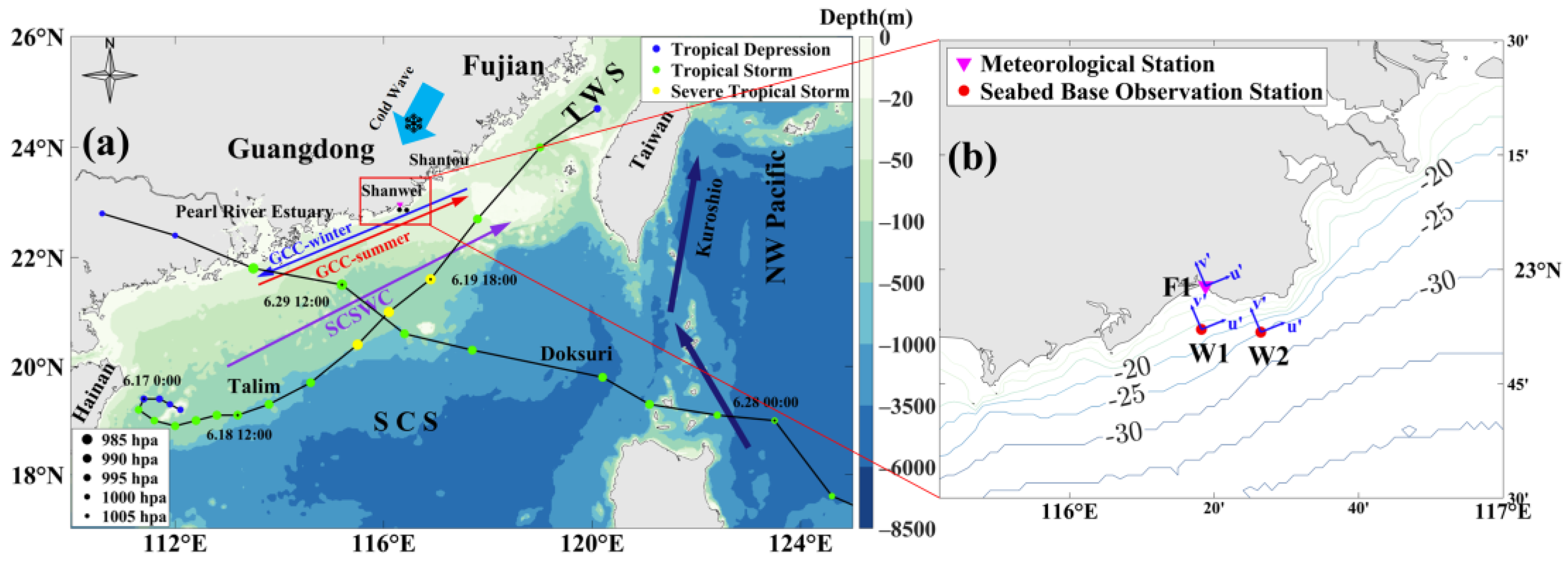
2.1.1. Study Area

The northern South China Sea (NSCS) has a broad continental shelf and a narrow continental slope, where complex and variable circulation prevails, influenced by dynamic factors, such as monsoons and Kuroshio [25]. Between the continental shelf and slope is the northeastward South China Sea Warm Current, whereas nearshore is a Guangdong coastal current that flows west in winter and reverses in summer. The study area was located in the shallow water area of the continental shelf in the NSCS, with a water depth of approximately 20 m. This is one of the major seasonal upwelling areas in China [26] and is subject to East Asian monsoon control throughout the year. Southwesterly winds prevail in summer, and surface water is transported offshore by upwelling due to the influence of the terrain and the Ekman effect [27,28]. Conversely, northeasterly winds prevail in winter, and under the influence of relaxed northerly or southerly winds, counterwind currents are found in the shelf waters of the NSCS [29,30]. Therefore, under the control of different monsoons, nearshore currents exhibit significant seasonal characteristics [31].

2.1.2. Observation and Satellite Remote Sensing Data

Two seabed-based observation stations (W1 and W2) were deployed along the eastern coast of Guangdong. The average water depths at W1 and W2 were 18.8 m and 22.3 m, and the coordinates were 22.863° N, 116.304° E and 22.869° N, 116.441° E respectively (Figure 1). Each station was equipped with acoustic wave and current profilers manufactured by Nortek to record currents, temperature, pressure, and echo intensity. The instruments were placed upward facing and had a 5 min sampling interval and a 1 MHz sampling frequency, with a burst duration of 6 Hz and bin size of 50 cm. The observation period of W1 was from 4 November 2011 to 20 December 2011 (winter) and 22 April 2012 to 3 July 2012 (summer), whereas that of W2 was from 22 December 2011 to 9 January 2011 (winter) and 22 April 2012 to 3 July 2012 (summer). In addition, concurrent wind, air pressure, and air temperature data were recorded by a meteorological station (F1) at a 10 min sampling interval in the study area.

The satellite remote sensing data used in this study include sea surface wind field (SSWF), sea surface current field (SSCF), and sea surface height (SSH). All data were obtained from the National Centers for Environmental Prediction (NCEP) Climate Forecast System Version 2 Product. The temporal and spatial resolutions were 1 h and 0.5°, respectively (https://rda.ucar.edu/datasets/ds094.1, accessed on 5 March 2024).

2.1.3. TCs and CWs

TC information (temporal resolution: 6 h), including longitude and latitude, minimum central pressure, and maximum wind speed, was obtained from the best track dataset of the Tropical Cyclone Data Center of the China Meteorological Administration (https://tcdata.typhoon.org.cn/, accessed on 14 June 2023). The TC (Talim and Doksuri) tracks are shown in Figure 1, and the development and the duration of impact on the study area are detailed below.

TC Talim (T1) formed east of Hainan Island in the SCS on 17 June 2012 and intensified into a tropical storm. T1 moved northeastward and reached the south side of the study area on 18 June, when it intensified into a severe tropical storm with a maximum wind speed of 25 m/s and a central pressure of 985 hPa. The 200 km level 7 wind circle continually covered the study area until T1 moved northeastward into the TWS and eventually dissipated on 19 June. TC Doksuri (T2), which formed in the NW Pacific Ocean, intensified into a tropical storm and moved northwestward to the NSCS on 26 June 2012. T2 reached the study area on 29 June, when it intensified into a severe tropical storm with a maximum wind speed of 23 m/s and a central pressure of 985 hPa. The 150 km level 7 wind circle continually covered the study area until T2 moved northwestward and eventually dissipated into Guangdong Province on 30 June.

A CW is a strong cooling weather process where large-scale cold air hits China from west of the Asian continent, which causes a large-scale range of strong cooling and is accompanied by wind, rain, and snow. It can also cause the temperature to drop rapidly by >8 °C in 24 h, with the lowest temperature reaching below 4 °C. However, the standards for CWs differ in different places because of the influence of the geographical environment and climatic conditions. In this study, three CW processes (C1, C2, and C3) were selected for the observation period based on meteorological data and CW standards, and they are shown in

Table 1. Information on TCs and CWs.

Event	Name	Duration (YYYY.MM.DD HH)	Max Wind Speed (m/s)	Min Central Pressure (hPa)
TC	T1	2012.06.17 20–2012.06.19 05	25	985
	T2	2012.06.26 08–2012.06.30 06	23	985
CW	C1	2011.11.06 07–2011.11.09 23	8.2	-
	C2	2011.11.19 15–2011.11.22 00	10.8	-
	C3	2011.12.24 22–2011.12.27 16	11.2	-

(www.cma.gov.cn/kppd/kppdsytj/201311/t20131126_232584.html, access on 7 May 2024).

2.2. Methods

2.2.1. Data Quality Control

Owing to the influences of wind, terrain, and other factors, the attitude of the base observation instrument may change to different degrees. Therefore, to ensure the accuracy and effectiveness of the data, the roll and pitch of the instrument were used to determine attitude. After data quality control, the roll and pitch angles were recorded by the clinometer within 5°, indicating that the instrument was in a vertical state during the observation and that the observation data were reliable and accurate. In addition, owing to instrument failure, the residual water level and bottom-water temperature at the W1 station in the summer were missing.

2.2.2. Harmonic Analysis and Axis Transform

As the eastern Guangdong coast is located in the northern shelf area of the SCS, the water level and current change periodically owing to tidal signals, which affect the TC and CW signals. Therefore, in this study, the classical harmonic analysis model (T_Tide toolbox [32]) was used to filter the observed current data, and the Lanczos cosine filter was used to filter the low-pass data for subsequent analysis [33].

The current and wind data were decomposed into east-west and north-south velocity components. As the direction of the shoreline near stations W1 and W2 was northeast-southwest, the coordinate axis was rotated by 22.5° to obtain the along-shore velocity (u’) and cross-shore velocity (v’). Positive values parallel to the isobaths represent the northeastward direction along the coast, and negative values represent the southwest direction.

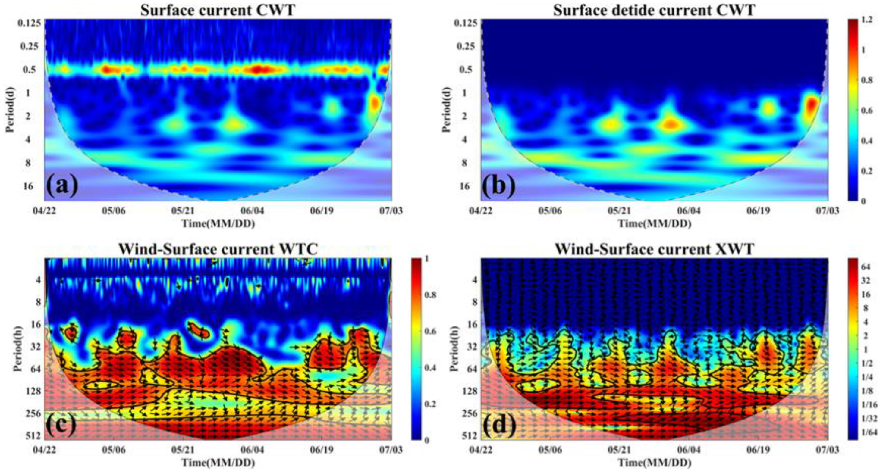
2.2.3. Wavelet Analysis

The continuous wavelet transform (CWT) can analyze time series data containing nonstationary power at many different frequencies [34]. The Morlet wavelet function was selected to conduct CWT on the time series data of surface alongshore current velocities before and after tide filtering and to obtain the wavelet power spectrum of the current. The formula used is as follows:

$$W_n^X\left(s\right)=\sqrt{{\displaystyle \frac{\delta t}{s}}}{\sum }_n^N{X}_n{\psi }_0^{\ast }\left[\right(n-n_1\left){\displaystyle \frac{\delta t}{s}}\right]$$

(1)

In Equation (1), $X_n$ represents the continuous wavelet transform of the time series (n = 1, 2, 3 …… N), $\ast$ represents complex conjugation, $s$ represents a smoothing operator in time and scale, $\delta t$ represents the time step, and ${\left|W_n^X\left(s\right)\right|}^2$ represents density of the wavelet energy spectrum.

Cross wavelet transform (XWT) is a signal analysis technique that combines wavelet transform and cross-spectrum analysis, which can be used to measure the power distribution of two signals [35]. The formula used is as follows:

$$W_{xy}=W_x^{\ast }{W}_y$$

(2)

In Equation (2), $W_x$ and $W_y$ represent the wavelet transforms of the two signals. The superscript * indicates a complex conjugate.

The wavelet coherent spectrum (WTC) can measure the local correlation closeness of two time series in the time-frequency space [36], defined as:

$${\rho }_{xy}={\displaystyle \frac{\left|s\left(W_{xy}\right)\right|}{{\left[s{\left(\left|W_x\right|\right)}^{2}s{\left(\left|W_y\right|\right)}^2\right]}^{1/2}}}$$

(3)

In Equation (3), ${\rho }_{xy}$ denotes the wavelet coherence, $W_{xy}$ denotes the wavelet cross-spectrum of two signals, and $s$ is a smoothing operator in time and scale. The phase of the wavelet cross-spectrum values can be used to identify the relative lag between two signals.

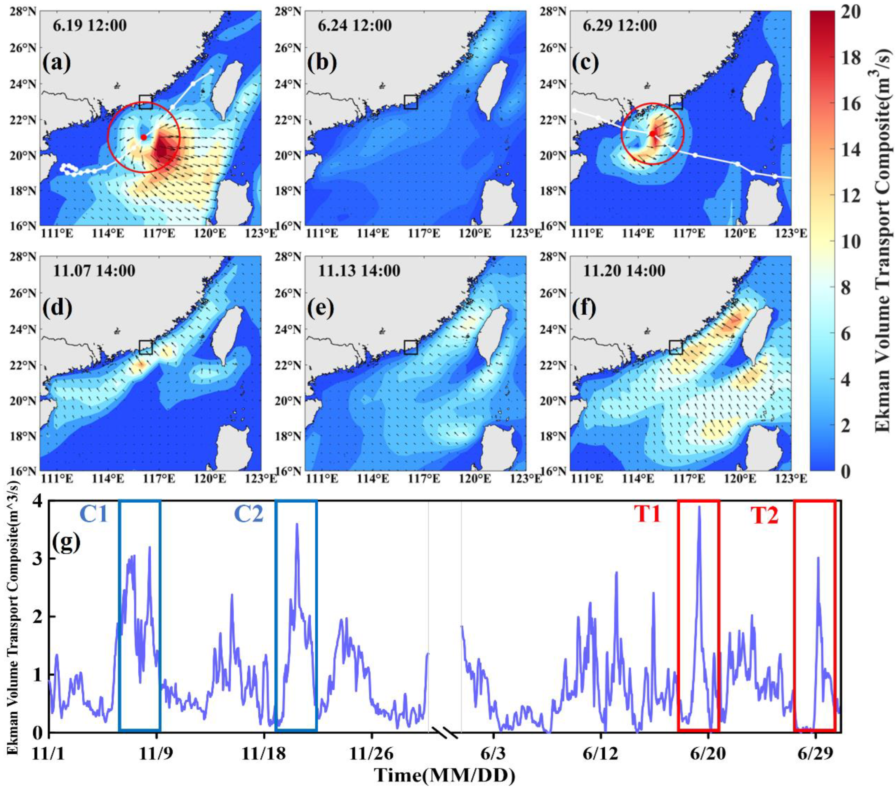
2.2.4. Ekman Volume Transport

To study water transport and marine environmental changes in coastal waters under the influence of TCs and CWs, we calculated the Ekman volume transport in the NSCS during T1 and T2 in summer and C1 and C2 in winter. The formula is as follows:

$$Q_x={\displaystyle \frac{Y{\tau }_y}{f\rho }}$$

(4)

$$Q_y=-{\displaystyle \frac{X{\tau }_x}{f\rho }}$$

(5)

$$\stackrel{\rightharpoonup }{{\tau }_x}={\rho }_a{C}_d\stackrel{\rightharpoonup }{u}\left|V\right|$$

(6)

$$\stackrel{\rightharpoonup }{{\tau }_y}={\rho }_a{C}_d\stackrel{\rightharpoonup }{v}\left|V\right|$$

(7)

$$\left|V\right|=\sqrt{u^2+v^2}$$

(8)

where $\rho$ is the density of seawater (1026 kg/m³); $f$ is the Coriolis parameter, $f=2\omega sin\left(\phi \right)$, $\omega =7.27\times {10}^{-5}{s}^{-2}$; X and Y are calculated for the width of the northbound and eastbound transport, respectively (unit width of 1 m is taken for this study); $Q_x$ and $Q_y$ are for the eastbound and northbound Ekman volume transport, respectively; $\stackrel{\rightharpoonup }{{\tau }_x}$ and $\stackrel{\rightharpoonup }{{\tau }_y}$ are for the eastbound and northbound wind stress, respectively; ${\rho }_a$ is for the air density (1.29 kg/m³); $C_d$ is the drag coefficient; and $\stackrel{\rightharpoonup }{u}$ and $\stackrel{\rightharpoonup }{v}$ are for the eastbound and northbound wind speeds, respectively, at the 10 m sea surface.

3. Results

3.1. Characteristics of Sea Surface Wind and Current Field in the NSCS During Observation

Figure 2 displays the variations in SSWF, SSCF, and SSHA in the NSCS before, during, and after TC. Before and after the TC’s passage, the NSCS was under the influence of the East Asian summer monsoon, with an average sea surface wind speed and current velocity of 5.2 m/s and 0.3 m/s, respectively. The nearshore water level anomaly was approximately −0.15 m, and the current flowed in a northeasterly direction (Figure 2c–f). As the TC formed and gradually approached the coast, it created a cyclonic circulation on the sea surface, leading to increases in wind speed and current velocity, reaching maxima of 25 m/s and 0.94 m/s, respectively. A notable rise in water level, about 0.14 m, formed on the right side of the TC track (Figure 2b,g).

Figure 3 illustrates the variations in SSWF, SSCF, and SSHA in the NSCS before, during, and after the CW. Before and after the CW’s passage, the NSCS was in a wind relaxation phase, with an average sea surface wind speed and current velocity of 4.49 m/s and 0.14 m/s, respectively. The nearshore water level decreased by approximately 0.1 m on average. The nearshore wind direction was northeasterly or a weak southerly wind, and the current flowed in a northeasterly direction (Figure 3a,c,d,f,g,i). During the CW’s passage, the NSCS was in a wind forcing phase, with significant increases in sea surface wind speed and current velocity, reaching maxima of 9.46 m/s and 0.83 m/s, respectively. The nearshore water level increased significantly, with an average rise of 0.22 m (Figure 3b,e,h).

3.2. Seasonal Characteristics of Meteorological and Hydrological Elements in the Eastern Guangdong Coast

3.2.1. Wind, Pressure, and Temperature

Coastal wind speed, wind direction, air temperature, and air pressure exhibited clear seasonal trends during the observation period (Figure 4). In summer, the wind direction in the study area fluctuated between southwest and northeast, with an average wind speed of 3.74 m/s and a standard deviation of 1.79 m/s (Figure 4a). The average air temperature was 26.8 °C, with a standard deviation of 2.0 °C and a warming trend at a rate of 0.1 °C/d, and the temperature dropped several times, with a maximum range of 8.2 °C. The pressure changed relatively smoothly and stayed below 1010 hPa (Figure 4b). In contrast, the winter wind direction in the study area was dominated by sustained northeasterly winds with sporadic southerly wind processes. During the observation period, the northeasterly wind intensified several times, with an average wind speed of 4.2 m/s and a standard deviation of 1.87 m/s, which was higher than that in summer (Figure 4c). The average temperature and the standard deviation in winter were 19.1 °C and 3.7 °C, respectively, and several large cooling processes were observed under the influence of strong cold air, with a maximum range of 11.3 °C and a cold trend at a rate of 0.2 °C/d. The average pressure was 1017 hPa, with a standard deviation of 4 hPa and a maximum of 1025 hPa, indicating an overall increasing trend at a rate of 0.1 hPa/d (Figure 4d).

During TCs and CWs, the wind speed increased significantly, and the temperature decreased significantly. The air pressure decreased in the TC; however, it both increased and decreased in the CW. The changes in the TC and CW are discussed in the next section.

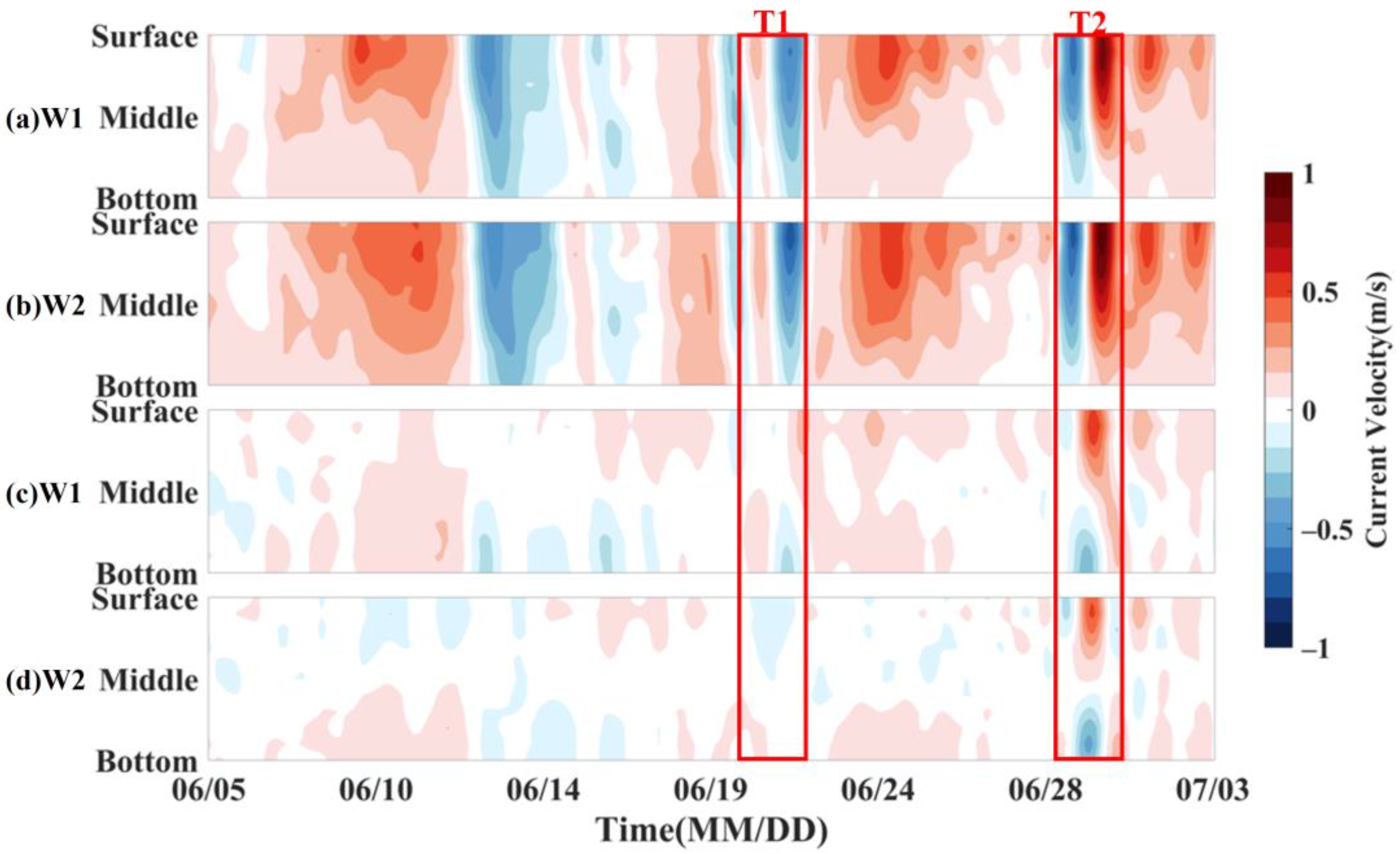
3.2.2. Current and Echo Intensity

Figure 5 shows that the southwesterly wind alternated with the northeasterly wind in summer, and the direction of the current followed this pattern. The variation trends of the summer current velocities at W1 and W2 were similar. Overall, the alongshore current velocity was an order of magnitude larger than the cross-shore current velocity, with average values of 0.2 m/s and 0.07 m/s and standard deviations of 0.07 m/s and 0.04 m/s, respectively. During the continuous seasonal southwesterly winds, the bottom layer presented a shore-oriented cross-shore current in summer, which was a typical upwelling structure (Figure 5c,d). In addition, during the observation period, there was a sustained northeasterly strong wind, and the maximum alongshore current velocities reached 0.82 m/s and 1.05 m/s at stations W1 and W2, respectively (Figure 5a,b).

Figure 6a,b show that the average alongshore current velocity in winter was 0.24 m/s and the average cross-shore current velocity was 0.1 m/s, with standard deviations of 0.07 m/s and 0.05 m/s, which were larger overall than those in summer. During the northeasterly wind strengthening, the current velocity increased significantly, and the maximum alongshore current velocity reached 1.02 m/s. The study area was mainly dominated by southwestward currents in winter, whereas during the relaxation of northerly or southerly winds, the alongshore current was dominated by the northeastward current, which may be the winter counterwind current phenomenon that exists in the nearshore sea.

The echo intensity of seawater reflects the particulate matter content and turbidity of the water body and can be used to indirectly reflect the source of the water body [37]. Considering the slightly different echo intensities of different instruments probes and the attachment of marine organisms, the echo intensity was only subjected to trend analysis rather than quantitative analysis. The overall characteristics of the echo intensity in summer and winter were similar, and a high value mainly appeared near the bottom. When the current was dominated by the southwestward current, the echo intensity was larger, whereas when it was dominated by the northeastward current, the echo intensity was smaller (Figure 5e,f and Figure 6c). This pattern was particularly significant during TCs and CWs, during which the current direction changed and the echo intensity increased; that is, the concentration of suspended solids increased, reflecting the material exchange process of the water bodies in the study area. In addition, the peak of the bottom echo intensity at the end of April and before the TC may be related to seasonal upwelling, while it may be affected by strong northeasterly winds in May, which caused bottom sediment resuspension. In winter, several forcing processes occurred in the northeasterly wind, which caused the strengthening of the southwestward current similar to the CW process, resulting in the increase in the bottom echo intensity.

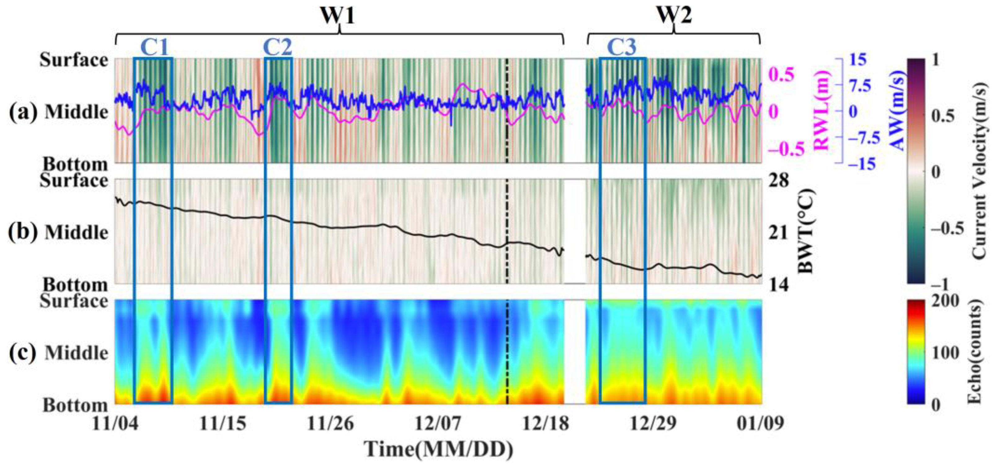
3.2.3. Bottom-Water Temperature and Residual Water Level

The residual water level displays prominent seasonal variation, primarily controlled by the prevailing alongshore wind. In the action stage of the southwesterly wind, the residual water level in the study area decreased by 0.2 m on average, whereas it increased by 0.15 m on average under the influence of strong northeasterly winds (Figure 5a). During TCs, the residual water level fluctuated significantly with a maximum range of 0.3 m owing to drastic changes in wind direction. Wintertime in the study area was dominated by northeasterly winds, leading to a general increase of 0.18 m on average in water levels throughout the observation period, with particularly notable increases during the CWs (Figure 6a).

The change in the bottom-water temperature reflects the exchange of cold and warm water, which also has obvious seasonal differences. The summer average bottom-water temperature was 24.9 °C, with a maximum of 25.6 °C and a minimum of 22.2 °C (Figure 5b). Conversely, the winter average was approximately 20.2 °C, with a maximum of 25.6 °C and a minimum of 14.8 °C (Figure 6b). The changes in the bottom-water temperature in winter and summer were closely related to the air temperature change trend. Overall, the bottom-water temperature in summer was in a seasonal warming state; however, it dropped several times during the observation period, which may be related to the intrusion of bottom water caused by upwelling. In winter, the bottom-water temperature in the study area remained in a seasonally cooled state during the observation period.

3.3. Variation in Meteorological and Hydrological Elements Caused by TCs and CWs

During TC events, the changes in hydrological and meteorological elements were correlated with the TC track and intensity (Figure 4 and Figure 5). When T1 passed through, the pressure dropped by 10 hPa, the lowest pressure reached 995 hPa, and the temperature rise trend was destroyed and dropped by 3.8 °C. The wind speed gradually increased when the TC passed through, with the maximum wind speed reaching 8.5 m/s (red box T1 in Figure 4a); the wind direction gradually changed to northeasterly. As the current direction changed to southwest, the current velocities at the W1 and W2 stations also increased, with maxima of 0.78 m/s and 0.95 m/s (red box T1 in Figure 7a,b). In addition, the upwelling structure at the bottom layer changed, and onshore transport changed to offshore transport. The coastal residual water level increased first and then decreased, with an increase of 0.1 m (Figure 5a). The bottom water stopped cooling and started warming at a rate of 0.2 °C/d owing to upwelling damage (Figure 5b). After the TC dissipated, the wind speed weakened and the wind direction gradually changed to southwest. The upwelling structure was restored, which caused a large amount of low-level cold water intrusion, and the cooling range reached 4.3 °C.

When T2 passed through, the pressure dropped by 4 hPa, the lowest pressure was 1000 hPa, and the temperature dropped by 2.1 °C. The maximum wind speed was 8.4 m/s (red box T2 in Figure 4a). The wind direction also changed to the northeast, and the maximum current velocities at the W1 and W2 stations were 1.01 m/s and 1.04 m/s (red box T2 in Figure 7a,b). The original upwelling structure was destroyed again, and the residual water level was raised by 0.3 m (Figure 5a) under the influence of the TC. The concentration of suspended matter from the surface to the bottom increased significantly, and the sediment was resuspended significantly during TC events.

CWs are generally divided into forcing and relaxation stages, in which the wind speed increases and decreases, respectively. During the CW forcing period (C1, C2, and C3), the local wind was a northeasterly wind with a continuous increase, the maximum wind speed was >8 m/s, and the wind speed varied by 6 m/s, 9.2 m/s, and 5.2 m/s, respectively. The maximum wind speed of C3 reached 11.2 m/s (Figure 4c). The temperature decreased by 8.9 °C, 8.1 °C, and 9 °C, respectively, and pressure decreased by 4 hPa during C1 and increased by 14 hPa and 4 hPa during C2 and C3, respectively (Figure 4d). In addition, the residual water levels increased by 0.2 m, 0.3 m, and 0.15 m, respectively. The bottom-water temperature showed a continuous decline, and the concentration of suspended matter in the bottom layer increased significantly, resulting in sediment resuspension (Figure 6a,b).

During the CW relaxation stage, the residual water level began to decrease slowly, the bottom-water temperature decreased, and the current velocity gradually decreased to the level present before the CW. At this point, the damanged original northeastward current structure in the study area during C1 did not recover, whereas the recovery trend was evident after C2 because of the influence of the relaxed southerly wind. In addition, the northeastward current structure existed only in the middle and lower layers after C3 and was conical (Figure 8a,c).

Furthermore, as depicted in the insets of Figure 2 and Figure 3, synchronous analysis and comparison were conducted on the SSCF, SSWF, and measured current and wind data off the coast of eastern Guangdong during both winter and summer observation periods. The results are presented in

Table 2. Comparison of reanalysis data with measured wind and current data during TCs and CWs (T1 and C1 are used as examples).

Data	Event	Main Wind Direction	Average Wind Speed (m/s)	Main Current Direction	Average Current Velocity (m/s)
Reanalysis Data 1	T1	NNE	3.08	SSW	0.26
	C1	NE	7.13	WSW	0.31
Measured Data 2	T1	NNE	3.56	SW	0.27
	C1	ENE	6.66	WSW	0.42

¹ The main wind and current direction of the reanalysis data are the direction with the greatest frequency of wind and current direction in the small plot areas in Figure 2 and Figure 3. ² The main wind and current direction of the measured data are the direction with the greatest frequency of wind and current direction of the stations in the same period.

. From the comparison of wind and current direction, it is evident that during TC and CW periods, there was a minor difference between the reanalysis and measured data in terms of wind and current directions, with the reanalysis data showing a slightly more northerly bias. When comparing wind speeds and current velocities, it could be observed that during TC, the measured values were higher than those from reanalysis, whereas during CW, the measured wind speeds were lower, but the current speeds are higher. Overall, during T1 and C1 periods, the reanalysis and measured data demonstrate good synchronicity. This study also validated processes such as T2, C2, and C3, yielding similar results to the aforementioned cases, indicating that the data can be used for subsequent discussion and analysis.

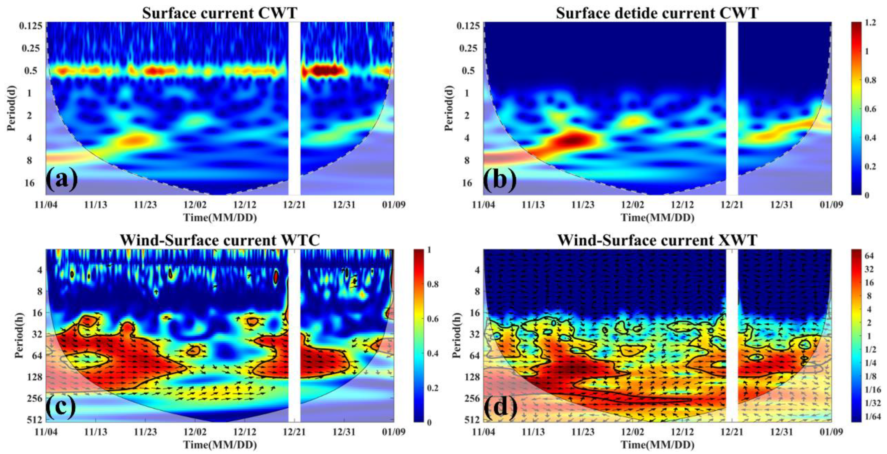
3.4. Wavelet Transform Analysis

During TCs and CWs, strong-wind stress can induce interaction between near-inertial waves and diurnal tides and generate energy, resulting in the generation of periodic signals [23] because the alongshore current velocity is an order of magnitude larger than the cross-shore current and is more significantly affected by wind. Therefore, wavelet analysis was used to obtain the time-frequency signals for the alongshore current in this study. As shown in Figure 9a,b, the summer surface current had a significant semi-diurnal tidal periodic signal that was significantly enhanced after removing the tidal signal. There were four obvious periodic signals during the observation period; the last two were T1 and T2. As can be seen from the time and frequency domains, T1 had a 1–2 d signal and 4 d duration, and T2 had a 1–3 d signal and lasted 5 d. Moreover, as seen in the wavelet coherence spectrum and cross-spectrum (Figure 9c,d), there were signal periods at 32–64 h and 16–64 h in T1 and T2, respectively, and the phase difference was 45° and 30°; there was still a signal above 128 h, and the phase difference was close to 0°.

In contrast to that in summer, the alongshore current exhibited three significant periodic signals corresponding to the three CWs in winter (Figure 10a,b). The results showed that a half-diurnal tide also existed in winter. The C1 had a 6–8 d signal and lasted for 12 d, whereas the C2, which was the most significant, had a 3–6 d signal and lasted for 10 d. The C3 signal, which had a 2–4 d signal and lasted for 10 d, was the weakest. As seen in the wavelet coherence spectrum and cross wavelet spectrum (Figure 10c,d), high energy appeared during the three CWs, and passed the significance test during the period of 32–256 h, indicating a good correlation between alongshore wind and surface current. C1 and C3 had strong energy at 32–256 h and 32–128 h, respectively, and the phase difference was 45°. C2 had significant energy at 32–256 h, and the phase difference was close to 0°.

In summary, the study area had significant semi-diurnal tide characteristics, and the periodic signals generated during summer TCs were relatively short and rapid, and relatively persistent during winter CWs. The phase difference also reflected the different lag times between the alongshore wind and current in different events, which is manifested as the speed of the response time.

4. Discussion

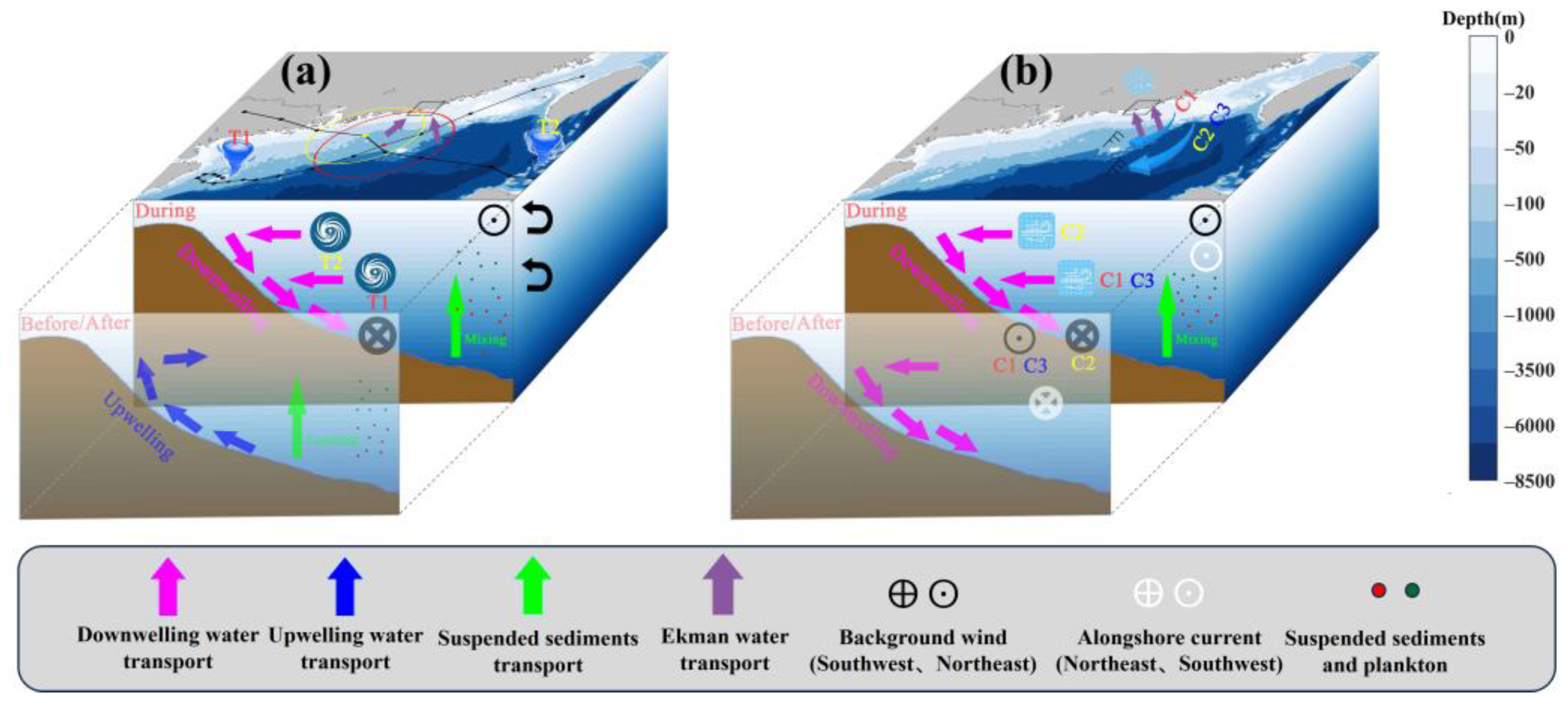
4.1. Mechanism of the Impact of TCs on Coastal Hydrological Elements

Seasonal upwelling along the eastern Guangdong coast in summer is an important part of the nearshore hydrodynamic process, and local wind field changes caused by TCs significantly impact the development of upwelling systems [38]. During the TC period, a positive wind curl is formed in the coastal water owing to the increase in wind stress (Figure 2b,g) [39], which drives the Ekman water onshore transport and causes a rise in the nearshore water levels, thus resulting in a southeasterly pressure gradient force perpendicular to the coast. Based on geostrophic equilibrium, the northwesterly Coriolis force increases, and the southwestward alongshore current is enhanced (red box in Figure 5a,b). In the bottom boundary layer, the enhanced alongshore current led to increased friction in the northeast direction, and as a result of the Ekman equilibrium, a greater southwesterly Coriolis force was required to balance the friction. Therefore, with the adjustment of local circulation to the abnormal wind induced by the TC, the accumulation of Ekman advection to the shore resulted in the occurrence of offshore currents in the middle and bottom waters, which inhibited the development of the original upwelling in the study area (Figure 5a,b). When the TC dissipated, the northeasterly wind weakened, which went against the formation of upwelling, and the local wind field was replaced by the prevailing southeasterly wind in summer, which drove the offshore Ekman transport of surface water. Moreover, the nearshore water level dropped and onshore compensation currents gradually formed in the bottom layer. With the rapid recovery of the upwelling systems, the intrusion of the underlying cold water was enhanced, resulting in a significant decrease in the bottom-water temperature. Therefore, abnormal changes in the bottom-water temperature can better reflect the characteristics of vertical upwelling [16].

The influence of TCs on coastal hydrodynamics depends on the TC’s track and intensity [40,41]. Owing to the influence of the Coriolis force, the wind stress on the right side of a TC track is often stronger than that on the left side when moving in the Northern Hemisphere [17]. In this study, T1 and T2 passed through the right and left sides of the study area, respectively, and the TCs had similar intensities. Due to the above-mentioned influence mechanism of TCs, the wind stress on T2 in the study area was stronger than that on T1, which resulted in a more significant increase in the water level in T2 than in T1. In addition, the influence of different TCs on the hydrodynamics was also reflected in the time-frequency signals, and the wavelet signal energy in T2 was more significant than that in T1 (Figure 9b). T1 and T2 differed in the correlation between the alongshore wind and surface alongshore currents, with phase differences of 45° and 30°, respectively. This shows that the alongshore current lags behind the alongshore wind for the 1/8 and 1/12 cycles (8 h and 5.3 h), respectively (Figure 9c,d), indicating that the current responds more rapidly to the TC (T2) with stronger wind stress.

In summary, the influence mechanism of the TC process on coastal hydrodynamics on the eastern Guangdong coast is as follows: TC transit causes changes in coastal wind, resulting in an abnormal rise and fall in coastal water levels, and then damages the cross-shore upwelling structure. The local wind is the main driving force, and the TC track is the main influencing factor.

4.2. Mechanism of the Impact of CWs on Coastal Hydrological Elements

CWs in winter are typically characterized by continuous oscillations between strong northeasterly winds and the duration of low pressure. When the CW passes through it, northeasterly winds dominate the NSCS (Figure 3b,e,h), and the wind direction changes minimally and does not generate a strong-wind stress curl [42]. Due to the Ekman effect, the enhanced northeasterly wind forms significant onshore transport, where seawater accumulates and generates an offshore pressure gradient force. Under the influence of geostrophic equilibrium, the northwesterly Coriolis force increases, and the southwestward alongshore current is enhanced; that is, the CW drives a strong and stable southwestward alongshore current (Figure 8a,c) [43]. Owing to the terrain and an increase in bottom friction, offshore current structures are formed at the middle bottom of the sea. When the CW enters the relaxation stage, the wind speed decreases rapidly, the nearshore water level begins to fluctuate, and the alongshore current gradually returns to the structure before the CW under the influence of the background wind field.

The intensity of the CW affects coastal hydrodynamic processes [44]. As shown in Figure 4c, the background wind field of C1 and C3 was relaxed north wind, whereas it was a relaxed southerly wind in C2, and the variation range of the wind speed followed the order C2 > C1 > C3. C1 and C3 were affected by the north wind for a long time; C1 had a low wind speed, and the residual water level fluctuated near the zero line. C3 had a high wind speed, and the residual water level remained above the zero line. However, C2 was affected by the southerly wind; the wind field was unstable, the wind speed changed significantly, and the residual water level presented the characteristics of a substantial increase and decrease (Figure 6a). The wavelet analysis showed that the C2 signal was the strongest, followed by that of C1, whereas that of C3 was the weakest. This corresponds to the variation amplitude of the wind speed, indicating that the coastal current was sensitive to the variation amplitude of wind speed during the CW (Figure 10b) [45]. The wavelet coherence and cross wavelet spectra showed similar characteristics (Figure 10c,d). The phase difference between C1 and C3 was approximately 45°, indicating that the coastal current lagged behind the coastal wind by 1/8 cycles (32 h and 16 h), which may have been due to the faster current response caused by the stronger intensity during C3. The C2 phase difference was close to 0°, indicating that the coastal current was positively correlated with the coastal wind and that the current responded more rapidly to the wind, which had a greater amplitude of change.

Therefore, the major mechanism by which the CW affects coastal hydrodynamics on the eastern Guangdong coast is that the northeasterly alongshore wind increases after a CW, resulting in a large increase in coastal water level, and the northeastward alongshore current structure is destroyed. Similarly, the local wind is the main driving force, and the CW intensity is the main influencing factor.

4.3. Comparison of the Mechanisms Between TCs and CWs on Coastal Marine Environment

In marine environments, extreme weather events, such as TCs and CWs, can cause drastic changes in air pressure, wind, and rainfall in a short time. Therefore, the increasing frequency of TCs and CWs may significantly change the hydrodynamics, sediment transport, and morphology on a short-term scale and have a significant impact on marine sediments and the ecological environment [46].

TCs significantly alter the magnitude and direction of water transport. During the TC, the water transport volume in the study was approximately 3–4 m³/s, the water transport volume was twice that amount before the TC, the water transport was distributed in a divergent manner, and the nearshore water transport was greatly enhanced. Figure 11a,c show that the influence of TCs on Ekman volume transport in the NSCS was typically asymmetrical, and the maximum transport rate occurred on the right side of the TC track because the wind stress on the right side of the TC in the northern hemisphere is often stronger than that on the left side, which can maximize the divergence of the sea surface [47]. TCs bring much precipitation, increase river flow, and carry part of the suspended matter into the coastal waters, causing the seawater to re-levitate, which is reflected in the increase in echo intensity. In addition, because the study area was located in the level 7 wind circle of T1 (mainly controlled by the cyclone field) and outside the level 7 wind circle of T2 (mainly controlled by the peripheral wind field), the water vapor on the right side of the TC was enhanced, resulting in the nearshore water level in T1 being markedly lower than that in T2. In addition, studies have shown that TCs with different tracks have similar impacts on the East China Sea Coastal Current, and TCs directly passing through the East China Sea have a greater impact on the nearshore processes, which cause strong coastal water transport and influence the dispersal path of sediment and freshwater [38,48]. Therefore, changes in wind and current may have a notable impact on nearshore water transport during TC [11].

Generally, the Ekman transport driven by the northeast monsoon in winter in the study area is manifested as surface onshore and bottom offshore, which is conducive to the offshore transport of nearshore materials [49]. During the CW, the water transport volume in the study area was approximately 2–3 m³/s, which was three times that amount before the CW, with a strengthened northeasterly wind. Water transport is distributed in a long strip to the shore under the influence of wind direction (Figure 11d,f,g). Owing to the differences in the intensities of C1 and C2, the water transport rates and ranges were different. Simultaneously, under the influence of the background wind field, the nearshore water level rose to different degrees during C1 and C2, indicating different cross-shore water transport volumes (Figure 6a). Relevant studies have shown that when cold air invades the northern waters of the Yangtze River Estuary and produces CWs, water transport caused by wind leads to the resuspension process of coastal seabed sediments, which has an important impact on ocean-related environmental changes [8]. Therefore, the water level fluctuation caused by alternating strong and weak winter winds can control the transport process of submesoscale water bodies, and a significant increase in shear stress near the bottom-water bodies leads to a large amount of submarine fine-grained sediment resuspension [50], thereby increasing the echo intensity near the bottom-water bodies (Figure 6c).

In the coastal waters of the NSCS, the effects of TCs and CWs on ocean dynamics were similar to some extent; however, clear differences were present. Both summer TCs and winter CWs can inject huge amounts of energy into the ocean, causing strong mixing of seawater, increasing the speed of the mixed laminar current and changing the structure, material composition, and transport volume of nearshore water bodies [51]. During TCs and CWs, strong-wind shear can cause drastic changes in ocean currents [52] and near-inertial oscillations of seawater and generate corresponding periodic signals. High-frequency changes generated during TCs and CWs coexist with topographic induction, which can cause water-level fluctuations in nearshore sea areas [53]. In addition, sediment resuspension occurs in the upper ocean, which increases the concentration of nearshore suspensions, resulting in geomorphic changes in the marine environment [54].

Although TCs and CWs are both extreme weather events, their effects on the eastern Guangdong coast are different. From a time perspective, TCs mainly occur in summer and autumn, from June to September. They are tropical cyclones produced on the tropical ocean surface, and their wind direction is complex and changeable. However, CWs, a process of large-scale strong cold air invasion to the south, mainly occur in winter and spring from November to February, and the wind direction remains unchanged [40,55]. As wind stress is one of the main driving forces of inshore currents, and the wind direction changes during TCs and CWs are different, the influence of the two on the change in current is completely different. TCs destroy the seasonal upwelling structure, causing the bottom cold water invasion process to stop and the abnormal rise and fall in nearshore water levels through wind stress curl and the Ekman effect (Figure 12a) [15]. Conversely, during CWs, the strengthening of the northeasterly wind affects the northeastward current structure along the coast and causes a rise in the nearshore water level through the Ekman effect (Figure 12b) [43]. In addition, the period and duration of the oscillation signals of the current are relatively short during TCs and relatively long during CWs, and the signal response speeds of both are significantly affected by wind.

5. Conclusions

In this study, we used the measured data collected in the NSCS, combined with remote sensing reanalysis data, to record TC and CW events and study the coastal hydrodynamic evolution process, influencing mechanisms, and marine environmental effects under the influence of TCs and CWs.

The results showed that the hydrological and local meteorological elements had significant seasonal characteristics. However, extreme weather events, such as TCs and CWs, disrupt the original variation trend; wind stress is the major driving force of coastal hydrodynamics, and the main influencing factors are the TC track and CW intensity. TCs are characterized by a large wind direction change, wind and current increase, and an increase in echo intensity. Although the wind direction changed minimally during the CW, it induced a phenomenon similar to that of the TC. However, their influencing mechanisms are significantly different. During the TC, the original seasonal upwelling structure and intrusion process of the underlying cold water were destroyed. The abnormal rise and fall in the nearshore water level were mainly related to the wind stress curl and Ekman effect, and the water transport was mainly concentrated on the right side of the TC track. When the CW passed through it, the original northeastward current structure was significantly affected, and the increase in the nearshore water level was related to the Ekman effect. Water transport was mainly concentrated in the nearshore strong-wind zone. In addition, the difference between TCs and CWs was also reflected in the time-frequency domain, with 1–3 d and 4–8 d signals, respectively; the TC signals were short and rapid, whereas the CW signals were more long-lasting.

This study enhanced our understanding of the response of coastal hydrodynamics to extreme weather events on the eastern Guangdong coast, and the results can provide references for disaster management and protection in coastal marine engineering and fishery engineering under extreme events. Because of the influence of cloud cover in extreme weather, remote sensing data for water color in nearshore areas are missing; therefore, a more precise numerical model to analyze and study marine environment changes, such as nearshore sediment transport, must be established.

References

- Kundzewicz, Z.W. Extreme Weather Events and their Consequences. Pap. Glob. Chang. IGBP 2016, 23, 59–69. [Google Scholar] [CrossRef]
- La Sorte, F.A.; Johnston, A.; Ault, T.R. Global trends in the frequency and duration of temperature extremes. Clim. Chang. 2021, 166, 1. [Google Scholar] [CrossRef]
- Wang, C.; Yao, Y.; Wang, H.; Sun, X.; Zheng, J. The 2020 Summer Floods and 2020/21 Winter Extreme Cold Surges in China and the 2020 Typhoon Season in the Western North Pacific. Adv. Atmos. Sci. 2021, 38, 896–904. [Google Scholar] [CrossRef] [PubMed]
- Wu, X.; He, Q.; Shen, J.; Peng, Z.; Guo, L.; Xie, W.; Lin, J. Different effects between cold front and tropical cyclone on short-term morphodynamics in the Changjiang Delta. J. Mar. Syst. 2024, 243, 103961. [Google Scholar] [CrossRef]
- Li, Y.; Xu, X.; Yin, X.; Fang, J.; Hu, W.; Chen, J. Remote-sensing observations of Typhoon Soulik (2013) forced upwelling and sediment transport enhancement in the northern Taiwan Strait. Int. J. Remote Sens. 2015, 36, 2201–2218. [Google Scholar] [CrossRef]
- Xu, X.; Gao, J.; Shi, Y.; Wu, X.; Lv, J.; Zhang, S.; Liu, S.; Liu, T.; Yang, G. Cross-Front Transport Triggered by Winter Storms Around the Shandong Peninsula, China. Front. Mar. Sci. 2022, 9, 975504. [Google Scholar] [CrossRef]
- Guan, S.; Zhao, W.; Huthnance, J.; Tian, J.; Wang, J. Observed upper ocean response to typhoon Megi (2010) in the Northern South China Sea. J. Geophys. Res. Ocean. 2014, 119, 3134–3157. [Google Scholar] [CrossRef]
- Tang, J.; Wang, Y.P.; Zhu, Q.; Jia, J.; Xiong, J.; Cheng, P.; Wu, H.; Chen, D.; Wu, H. Winter storms induced high suspended sediment concentration along the north offshore seabed of the Changjiang estuary. Estuar. Coast. Shelf Sci. 2019, 228, 106351. [Google Scholar] [CrossRef]
- Wang, T.; Jin, S.; Wang, K. Analysis of the Temporal and Spatial Development of Cold Waves in Fujian Province over the Last 58 Years. J. Phys. Conf. Ser. 2024, 2706, 012071. [Google Scholar] [CrossRef]
- Chen, W.; Tong, Y.; Li, W.; Ding, Y.; Li, J.; Wang, W.; Shi, P. Interannual Variations in the Summer Coastal Upwelling in the Northeastern South China Sea. Remote Sens. 2024, 16, 1282. [Google Scholar] [CrossRef]
- Jin, W.; Liang, C.; Tian, X.; Hu, J.; Ding, T.; Zhou, B.; Chen, X.; Wang, Y. Identifying Oceanic Responses with Validated Satellite Observations after the Passage of Typhoons in the Northern South China Sea. Remote Sens. 2022, 14, 3872. [Google Scholar] [CrossRef]
- Cai, S.; Jing, C.; Xu, J. Response of upwelling in eastern Guangdong and southern Fujian coastal seas to the local wind variation. Haiyang Xuebao 2016, 38, 1–12, (In Chinese with English Abstract). [Google Scholar]
- Niu, Y.; Xu, Z.; Hao, Z.; You, J.; Yin, B.; Meng, X. Observed near-inertial waves generated by tropical and extratropical cyclones in the East China Sea. J. Sea Res. 2023, 196, 102458. [Google Scholar] [CrossRef]
- Shi, W.; Huang, Z.; Hu, J. Using TPI to Map Spatial and Temporal Variations of Significant Coastal Upwelling in the Northern South China Sea. Remote Sens. 2021, 13, 1065. [Google Scholar] [CrossRef]
- Zheng, B.; Li, Y.; Li, J.; Shu, F.; He, J. Impact of tropical cyclones on the evolution of the monsoon-driven upwelling system in the coastal waters of the northern South China Sea. Ocean Dyn. 2017, 68, 223–237. [Google Scholar] [CrossRef]
- Pan, A.; Guo, X.; Xu, J.; Huang, J.; Wan, X. Responses of Guangdong coastal upwelling to the summertime typhoons of 2006. Sci. China Earth Sci. 2011, 55, 495–506. (In Chinese) [Google Scholar] [CrossRef]
- Zhang, H.; He, H.; Zhang, W.-Z.; Tian, D. Upper ocean response to tropical cyclones: A review. Geosci. Lett. 2021, 8, 1. [Google Scholar] [CrossRef]
- Yin, L.; Qiao, F.; Zheng, Q. Coastal-Trapped Waves in the East China Sea Observed by a Mooring Array in Winter 2006. J. Phys. Oceanogr. 2014, 44, 576–590. [Google Scholar] [CrossRef]
- Guan, B.; Fang, G. Winter Counter-wind Currents off the Southeastern China Coast: A Review. J. Oceanogr. 2006, 62, 1–24. [Google Scholar] [CrossRef]
- Chen, Y.; Cao, Y.; Liao, S.; Ma, Y.; Liu, Y.; Ouyang, Y.; Xiang, R. Observational Analysis of the Formation Reasons and Evolution Law of Winter Counter-Wind Current in Jiazi Sea Area of Northeastern South China Sea. J. Mar. Sci. Eng. 2022, 10, 893. [Google Scholar] [CrossRef]
- Huang, D.; Zeng, D.; Ni, X.; Zhang, T.; Xuan, J.; Zhou, F.; Li, J.; He, S. Alongshore and cross-shore circulations and their response to winter monsoon in the western East China Sea. Deep Sea Res. Part II Top. Stud. Oceanogr. 2016, 124, 6–18. [Google Scholar] [CrossRef]
- Lin, L.; Wang, Y.; Liu, D. Vertical average irradiance shapes the spatial pattern of winter chlorophyll-a in the Yellow Sea. Estuar. Coast. Shelf Sci. 2019, 224, 11–19. [Google Scholar] [CrossRef]
- Liu, J.; He, Y.; Li, J.; Cai, S.; Wang, D.; Huang, Y. Cases Study of Nonlinear Interaction Between Near-Inertial Waves Induced by Typhoon and Diurnal Tides Near the Xisha Islands. J. Geophys. Res. Ocean. 2018, 123, 2768–2784. [Google Scholar] [CrossRef]
- Yang, Z.; Lei, K.; Guo, Z.; Wang, H. Effect of a Winter Storm on Sediment Transport and Resuspension in the Distal Mud Area, the East China Sea. J. Coast. Res. 2007, 232, 310–318. [Google Scholar] [CrossRef]
- Chang, M.H.; Lien, R.C.; Lamb, K.G.; Diamessis, P.J. Long-Term Observations of Shoaling Internal Solitary Waves in the Northern South China Sea. J. Geophys. Res. Ocean. 2021, 126, e2020JC017129. [Google Scholar] [CrossRef]
- Hu, J.; Wang, X.H. Progress on upwelling studies in the China seas. Rev. Geophys. 2016, 54, 653–673. [Google Scholar] [CrossRef]
- Gan, J.; Cheung, A.; Guo, X.; Li, L. Intensified upwelling over a widened shelf in the northeastern South China Sea. J. Geophys. Res. Ocean. 2009, 114, C09019. [Google Scholar] [CrossRef]
- Gan, J.; Li, L.; Wang, D.; Guo, X. Interaction of a river plume with coastal upwelling in the northeastern South China Sea. Cont. Shelf Res. 2009, 29, 728–740. [Google Scholar] [CrossRef]
- Shen, J.; Zhang, J.; Qiu, Y.; Li, L.; Zhang, S.; Pan, A.; Huang, J.; Guo, X.; Jing, C. Winter counter-wind current in western Taiwan Strait: Characteristics and mechanisms. Cont. Shelf Res. 2019, 172, 1–11. [Google Scholar] [CrossRef]
- Wang, D.; Hong, B.; Gan, J.; Xu, H. Numerical investigation on propulsion of the counter-wind current in the northern South China Sea in winter. Deep Sea Res. Part I Oceanogr. Res. Pap. 2010, 57, 1206–1221. [Google Scholar] [CrossRef]
- Bao, X.; Hou, Y.; Chen, C.; Chen, F. Analysis of characteristics and mechanism of current system on the west coast of Guangdong of China in summer. Acta Oceanol. Sin. 2005, 24, 5–13. [Google Scholar]
- Pawlowicz, R.; Beardsley, B.J.; Lentz, S.J. Classical tidal harmonic analysis including error estimates in MATLAB using T_TIDE. Comput. Geosci. 2002, 28, 929–937. [Google Scholar] [CrossRef]
- Duchon, C.E. Lanczos Filtering in One and Two Dimensions. J. Appl. Meteorol. 1979, 18, 1016–1022. [Google Scholar] [CrossRef]
- Grinsted, A.; Moore, J.C.; Jevrejeva, S. Application of the cross wavelet transform and wavelet coherence to geophysical time series. Nonlinear Process. Geophys. 2004, 11, 561–566. [Google Scholar] [CrossRef]
- Lafrenière, M.; Sharp, M. Wavelet analysis of inter-annual variability in the runoff regimes of glacial and nival stream catchments, Bow Lake, Alberta. Hydrol. Process. 2003, 17, 1093–1118. [Google Scholar] [CrossRef]
- Torrence, C.; Compo, G.P. A Practical Guide to Wavelet Analysis. Bull. Am. Meteorol. Soc. 1998, 79, 61–78. [Google Scholar] [CrossRef]
- Dwinovantyo, A.; Manik, H.M.; Prartono, T.; Susilohadi, S. Quantification and Analysis of Suspended Sediments Concentration Using Mobile and Static Acoustic Doppler Current Profiler Instruments. Adv. Acoust. Vib. 2017, 2017, 4890421. [Google Scholar] [CrossRef]
- Chi, W.; Shu, F.; Lin, Y.; Li, Y.; Luo, F.; He, J.; Chen, Z.; Zou, X.; Zheng, B. Typhoon-induced destruction and reconstruction of the coastal current system on the inner shelf of East China Sea. Cont. Shelf Res. 2023, 255, 104912. [Google Scholar] [CrossRef]
- Chelton, D.B.; Schlax, M.G.; Samelson, R.M.; de Szoeke, R.A. Global observations of large oceanic eddies. Geophys. Res. Lett. 2007, 34, L15606. [Google Scholar] [CrossRef]
- Guan, S.; Zhao, W.; Sun, L.; Zhou, C.; Liu, Z.; Hong, X.; Zhang, Y.; Tian, J.; Hou, Y. Tropical cyclone-induced sea surface cooling over the Yellow Sea and Bohai Sea in the 2019 Pacific typhoon season. J. Mar. Syst. 2021, 217, 103509. [Google Scholar] [CrossRef]
- Zhang, H.; Chen, D.; Zhou, L.; Liu, X.; Ding, T.; Zhou, B. Upper ocean response to typhoon Kalmaegi (2014). J. Geophys. Res. Ocean. 2016, 121, 6520–6535. [Google Scholar] [CrossRef]
- Mo, D.; Hou, Y.; Li, J.; Liu, Y. Study on the storm surges induced by cold waves in the Northern East China Sea. J. Mar. Syst. 2016, 160, 26–39. [Google Scholar] [CrossRef]
- Yu, Z.; Metzger, E.J.; Fan, Y. Generation mechanism of the counter-wind South China Sea Warm Current in winter. Ocean Model. 2021, 167, 101875. [Google Scholar] [CrossRef]
- Li, J.; Zheng, Q.; Hu, J.; Xie, L.; Zhu, J.; Fan, Z. A case study of winter storm-induced continental shelf waves in the northern South China Sea in winter 2009. Cont. Shelf Res. 2016, 125, 127–135. [Google Scholar] [CrossRef]
- Xuan, J.; Ding, R.; Ni, X.; Huang, D.; Chen, J.; Zhou, F. Wintertime Submesoscale Offshore Events Overcoming Wind-Driven Onshore Currents in the East China Sea. Geophys. Res. Lett. 2021, 48, e2021GL095139. [Google Scholar] [CrossRef]
- Wang, G.; Ling, Z.; Wang, C. Influence of tropical cyclones on seasonal ocean circulation in the South China Sea. J. Geophys. Res. Ocean. 2009, 114, C10022. [Google Scholar] [CrossRef]
- Li, W.; Wang, Z.; Lee, G.-h.; Huang, H. Ecological and sediment dynamics response to typhoons passing from the east and west sides of the Changjiang (Yangtze River) Estuary and its adjacent sea area. Mar. Geol. 2024, 467, 107188. [Google Scholar] [CrossRef]
- Deng, B.; Zhang, J.; Wu, Y. Recent sediment accumulation and carbon burial in the East China Sea. Glob. Biogeochem. Cycles 2006, 20, GB3014. [Google Scholar] [CrossRef]
- Shi, Y.; Gao, J.; Sheng, H.; Du, J.; Jia, J.; Wang, Y.; Li, J.; Bai, F.; Chen, Y. Cross-Front Sediment Transport Induced by Quick Oscillation of the Yellow Sea Warm Current: Evidence From the Sedimentary Record. Geophys. Res. Lett. 2019, 46, 226–234. [Google Scholar] [CrossRef]
- Liu, T.; Shi, Y.; Xu, X.; Liu, S.; Lyu, J.; Zhang, S.; Yang, G.; Ren, C.; Sheng, H.; Gao, J. Winter storms drive offshore transport and modulate phytoplankton blooms in Northern Taiwan, China. J. Hydrol. 2023, 627, 130391. [Google Scholar] [CrossRef]
- Wang, P.; Sheng, J. A comparative study of wave-current interactions over the eastern Canadian shelf under severe weather conditions using a coupled wave-circulation model. J. Geophys. Res. Ocean. 2016, 121, 5252–5281. [Google Scholar] [CrossRef]
- Niu, Y.; Guo, B.; Subrahmanyam, M.V.; Xue, B.; Ye, Y. The Influence of Typhoon “MITAG” on Waves and Currents in Zhoushan Sea Area, China. Atmosphere 2021, 12, 1027. [Google Scholar] [CrossRef]
- Wu, J.; Xue, X.; Hoffmann, L.; Dou, X.; Li, H.; Chen, T. A case study of typhoon-induced gravity waves and the orographic impacts related to Typhoon Mindulle (2004) over Taiwan. J. Geophys. Res. Atmos. 2015, 120, 9193–9207. [Google Scholar] [CrossRef]
- Lu, J.; Jiang, J.; Li, A. Differences in sedimentary dynamic processes between summer typhoons and winter cold waves on the inner shelf of the East China Sea: Insights from in-situ observations. Mar. Geol. Quat. Geol. 2023, 43, 96–105, (In Chinese with English Abstract). [Google Scholar]
- Xuan, J.; Huang, D.; Pohlmann, T.; Su, J.; Mayer, B.; Ding, R.; Zhou, F. Synoptic fluctuation of the Taiwan Warm Current in winter on the East China Sea shelf. Ocean Sci. 2017, 13, 105–122. [Google Scholar] [CrossRef]