Abstract
Underwater Acoustic Target Recognition (UATR) plays a crucial role in underwater detection devices. However, due to the difficulty and high cost of collecting data in the underwater environment, UATR still faces the problem of small datasets. Few-shot learning (FSL) addresses this challenge through techniques such as Siamese networks and prototypical networks. However, it also suffers from the issue of overfitting, which leads to catastrophic forgetting and performance degradation. Current underwater FSL methods primarily focus on mining similar information within sample pairs, ignoring the unique features of ship radiation noise. This study proposes a novel cross-domain contrastive learning-based few-shot (CDCF) method for UATR to alleviate overfitting issues. This approach leverages self-supervised training on both source and target domains to facilitate rapid adaptation to the target domain. Additionally, a base contrastive module is introduced. Positive and negative sample pairs are generated through data augmentation, and the similarity in the corresponding frequency bands of feature embedding is utilized to learn fine-grained features of ship radiation noise, thereby expanding the scope of knowledge in the source domain. We evaluate the performance of CDCF in diverse scenarios on ShipsEar and DeepShip datasets. The experimental results indicate that in cross-domain environments, the model achieves accuracy rates of 56.71%, 73.02%, and 76.93% for 1-shot, 3-shot, and 5-shot scenarios, respectively, outperforming other FSL methods. Moreover, the model demonstrates outstanding performance in noisy environments.
1. Introduction
Underwater Acoustic Target Recognition (UATR) is a challenging and significant area of research in passive sonar, playing a crucial role in both economic development and military security [1,2]. From an economic perspective, UATR technology can be applied to marine resource development, seabed exploration, and marine environmental protection. From a military standpoint, it enables the timely acquisition of target information such as enemy ships, assisting commanders in accurately assessing the battlefield situation and making informed decisions.
Given the complex and dynamic marine environment, numerous researchers have been dedicated to developing various UATR methods. The current UATR methods can be categorized into two main types. The first category utilizes manually extracted hydroacoustic data features for target recognition. For instance, Zhang et al. [3] employed the MFCC and utilized a backpropagation network for classification. Zhu et al. [4] improved network performance by analyzing the spectral components of ship-radiated noise through the extraction of different frequency band spectral features. Other features include wavelet decomposition [5,6,7] and sparse time–frequency representation [8,9].
The second category employs deep learning techniques for target recognition. With the continuous advancement of deep learning technology, deep neural networks have become widely used in UATR. Doan et al. [10] utilized time-domain signals as inputs to a dense convolutional neural network, achieving superior results at a 0 dB signal-to-noise ratio. Hong et al. [11] proposed 3D fusion features for target classification using ResNet18. Yang et al. [12] designed a lightweight squeezing and residual network under a ResNet architecture to ensure recognition accuracy while compressing the model. Jin et al. [13] utilize raw time-domain data as input to the model and incorporate an attention mechanism in a convolutional neural network to identify different types of ships. Inspired by visual transformers, Li et al. [14] incorporated transformers into UATR for the first time, comparing the performance of three features: short-time Fourier transform (STFT), filter bank (FBank), and mel-frequency cepstrum coefficients (MFCCs). They enhanced model training stability through pre-training on image and speech datasets and applying time and frequency masking for data augmentation.
While these deep learning-based methods have shown effectiveness in UATR, their performance may deteriorate or become invalid when faced with limited hydroacoustic data samples in practical situations. In recent years, researchers have employed data augmentation and deep generative adversarial networks to address the issue of limited samples in deep learning. Zhang introduced a data augmentation method based on generative adversarial networks [15]. Luo et al. [16] designed a conditional deep convolutional generative adversarial network for high-quality data augmentation, extracting multiple features of ship-radiated noise by generating spectrograms with different resolutions through a multi-window spectral analysis method. Gao combined DCGAN [17] and DenseNet [18] to overcome the limited sample constraint in UATR [19]. However, a significant knowledge gap still exists between generated samples and real samples, hindering their deployment in real underwater environments.
Few-shot learning (FSL) has emerged as a solution for recognizing new classes with limited samples and has demonstrated excellent capabilities in computer vision and speech domains. In the field of speech, Wang et al. [20] introduced a hybrid attention module combined with a prototype network for sound classification with fewer samples. Wang et al. [21] proposed a few-shot music source separation method using a small number of audio examples from the target instrument to adapt the U-Net model. You et al. [22] combined audio spectrogram transformers, data augmentation mechanisms, and conductive inference for sound event detection. FSL has also found successful applications in underwater tasks. Chen achieved underwater acoustic target recognition using an FSL approach with Siamese networks [23]. Xue introduced a semi-supervised learning approach to address the recognition challenge posed by limited samples [24]. Two metric learning-based approaches were investigated for sonar image classification, allowing the model to generalize to classes with fewer samples without extensive retraining [25]. Nie proposed a contrastive learning method for ship recognition with limited samples by comparing the similarity between pairs of positive and negative samples [26]. Tian utilized unlabeled samples and a small number of labeled samples to accomplish UATR, proposing a semi-supervised fine-tuning method to enhance model performance [27]. However, current FSL methods do not effectively utilize the specific characteristics of ship-radiated noise in UATR and may suffer from performance degradation due to differences between source and target domains. Moreover, these methods are prone to overfitting when fine-tuning is repeatedly performed with limited samples.
In this paper, we present a novel cross-domain contrastive learning-based few-shot underwater acoustic target recognition method (CDCF) to address the issue of overfitting in few-shot UATR models. Traditional FSL divides UATR into two stages: pre-training and fine-tuning. The pre-training phase involves training the model on source domain data to obtain a pre-trained feature extractor. In the fine-tuning phase, the feature extractor is fine-tuned using target domain data. We introduce self-supervised training during the fine-tuning stage to enhance the fine-tuning process by utilizing samples from the source domain. Additionally, we propose a base contrastive module to measure the similarity of corresponding frequency bands between augmented view samples. By leveraging contrastive self-supervised learning, CDCF efficiently extracts more fine-grained ship noise features. Including samples from the source domain during fine-tuning alongside the target domain samples enhances adaptability through gradual knowledge transfer and integration. We evaluate our method on two datasets, ShipsEar and DeepShip, to demonstrate its effectiveness. The main contributions of this paper are as follows:
- (1)
- We propose a novel cross-domain contrastive learning-based few-shot underwater acoustic target recognition method (CDCF) to address the overfitting problem in FSL approaches. The effectiveness of CDCF is validated through extensive experiments conducted on two publicly available datasets.
- (2)
- During the fine-tuning process, we incorporate a self-supervised training branch to assist in the fine-tuning procedure. By feeding the samples from target domains and a subset of samples from source domains into this branch, knowledge can be efficiently transferred from the source to the target domain during the fine-tuning process, facilitating the model’s adaptation to the new domain.
- (3)
- We introduce a frequency band contrastive module aimed at extracting fine-grained ship noise features, and we validate its effectiveness in real-world scenarios.
2. System Overview
2.1. Variable Definitions and Explanations
In few-shot learning, a model is first pre-trained on a large-scale base dataset, denoted as . The model is then fine-tuned on a support set, denoted as , from a novel dataset , allowing the model to generalize to previously unseen classes. Finally, the model’s performance is evaluated on a query set, denoted as , from .
In the aforementioned few-shot learning procedure, represents the base set, while denotes the novel set. Here, and refer to the samples in the base set and novel set, respectively. Similarly, and represent the corresponding labels for the samples in the base set and novel set. and indicate the sizes of the base and novel sets, signifying the number of samples in each dataset. Importantly, is significantly larger than . Furthermore, let denote the label space of the base set, meaning , and denote the label space of the novel set, implying . It is assumed that and are disjoint, i.e., .
During the fine-tuning process, a pre-trained model is adapted to accommodate the support set , which consists of N novel classes with K samples per class. Here, and denote the samples and labels in the support set, respectively, and represents the label space of the support set. Subsequently, the performance of the model is evaluated using the query set , which is also a subset of . and represent the samples and their corresponding labels in the query set. indicates the label space of the query set. Moreover, let and denote the label spaces of the support set and the query set, respectively. It should be noted that the classes in the support set and the query set are the same, i.e., . However, the samples in the support set and the query set are distinct.
2.2. General Formulation of Few-Shot UATR
In this section, we provide a detailed overview of the traditional FSL methods. Typically, traditional FSL methods consist of two stages: pre-training and fine-tuning. The model architecture is illustrated in Figure 1.
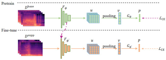
Figure 1.
Traditional few-shot learning framework. The model consists of two phases: pre-training and fine-tuning. In the pre-training stage, the feature extractor and classifier are trained on the source domain dataset. In the fine-tuning stage, the parameters of the feature extractor are transferred from , while the parameters of the classifier are randomly initialized. Fine-tuning is performed for the target domain.
During the pre-training stage, the model is trained using the source domain data, denoted as . The model takes various features of the data, such as STFT, MFCC, mel spectrograms, etc., as inputs. Through a feature extractor , high-dimensional features are extracted from the input data, resulting in a feature mapping . The formulation can be expressed as follows:
Subsequently, a pooling layer is applied to aggregate the features, yielding a feature embedding . The pooling operation can be represented as follows:
The final classification results are generated through a classifier , which takes the feature embedding v as input. Mathematically, it can be described as
Finally, the cross-entropy loss function is utilized to compute the loss and update the parameters of the feature extractor.
In the fine-tuning stage, the model architecture remains the same as in the pre-training stage. However, the parameters of the feature extractor are transferred from the pre-training stage’s feature extractor , while the parameters of the classifier are initialized randomly. The model is fine-tuned using the target domain data . Again, the cross-entropy loss function is employed to calculate the loss and update the parameters of and . To simplify the expression, the formulation can be expressed as
Finally, the performance of the model is evaluated on using the fine-tuned parameters and .
2.3. CDCF Model
The previous section introduces traditional FSL, which demonstrates remarkable capabilities in computer vision domains. However, in underwater environments, data samples are severely limited, and repeated model fine-tuning can potentially lead to overfitting. Moreover, the collected data are often affected by noise conditions, which vary across different hydrological environments, resulting in significant disparities between the source and target domains and, consequently, a decline in model performance. In light of these challenges, we propose CDCF. The model architecture is depicted in Figure 2.
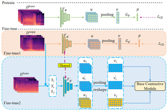
Figure 2.
Overall framework for CDCF. In the pre-training phase, the model comprises a feature extractor and a classifier , trained on the source domain dataset. In the fine-tuning stage, the feature extractor initiates its parameters from and subsequently adapts to the novel domain by self-supervised learning in positive and negative sample pairs.
Diverging from traditional FSL, we incorporate a self-supervised training branch during the fine-tuning stage to facilitate the fine-tuning process. Simultaneously, we introduce a frequency band contrast loss to assess the similarity between corresponding frequency bands in the enhanced views of the samples, enabling the model to capture more refined features. The CDCF model comprises two stages: pre-training and fine-tuning. The pre-training stage aligns with the traditional FSL illustrated in Figure 1. The classifier in CDCF employs fully connected layers. During the fine-tuning stage, CDCF consists of two branches: Fine-tune1, representing the traditional FSL fine-tuning branch, and Fine-tune2, representing the self-supervised training branch with the frequency band contrast loss. To ensure clarity, we focus on elaborating on the fine-tuning stage of CDCF.
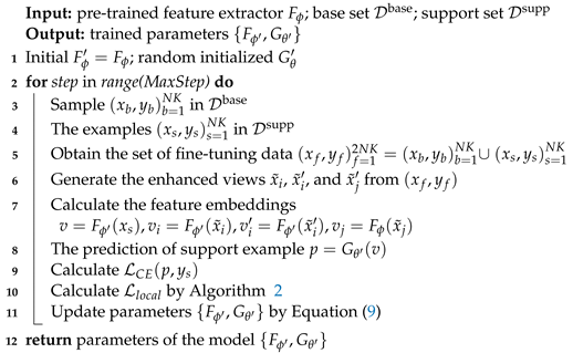
Similar to traditional FSL methods, in the fine-tuning stage of CDCF, the parameters of the feature extractor in both branches are transferred from the pre-training stage. Moreover, the parameters of the feature extractor are shared between the Fine-tune1 and Fine-tune2 branches. The settings in the Fine-tune1 branch remain the same as shown in Figure 1. For the Fine-tune2 branch, unlike traditional fine-tuning that only utilizes samples from , we aim to accelerate the model’s adaptation to the target domain by using samples from both and a subset of samples from . Mel spectrograms are used as input to the model, and two augmented views ( and ) are generated from the mel spectrogram of one sample, while another augmented view () is generated from the mel spectrogram of another sample. The augmentation methods and analysis are described in Section 3.2. These augmented views are fed into the feature extractor , resulting in feature maps , , with dimensions . Subsequently, these feature maps are processed through pooling and reshape operations, yielding feature embeddings , , with dimensions . Finally, these feature embeddings are input to the base contrastive module (illustrated in Section 2.4) to compute the frequency band contrast loss. The overall algorithm implementation is presented in Algorithm 1.
| Algorithm 1: Overall training algorithm. |
 |
We posit that the underlying intuition behind model enhancement lies in leveraging contrastive learning to broaden the knowledge scope of the source domain through pairs of augmented samples generated using arbitrary enhancement techniques. This approach concurrently preserves the model’s capacity to extract universal features during the pre-training stage and provides a certain degree of mitigation against overfitting.
2.4. Base Contrastive Module
Contrastive learning is a crucial component of self-supervised learning and has diverse applications in tasks such as identification [28] and detection [29]. In traditional contrastive learning, the mel spectrogram of the ship signal after obtaining the enhanced view is fed to the feature extractor in the Fine-tune2 branch. It produces feature maps , , with dimensions of . These feature maps are then processed using pooling and reshape operations to generate feature embeddings , , with a dimension of C. The similarity between the feature embeddings of different positive and negative sample pairs is compared. In contrast to traditional contrastive learning methods, our proposed frequency bands contrastive learning generates feature embeddings with a dimension of , as described in Section 2.3. Specifically, we compare the similarities between corresponding frequency bands of positive and negative sample pairs. This comparison is illustrated in Figure 3.
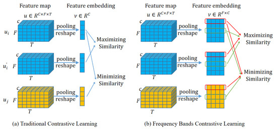
Figure 3.
Comparison between two contrastive learning methods.
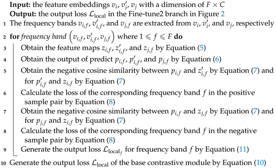
Based on the frequency bands contrastive approach illustrated in Figure 3b, we propose a base contrastive module, as depicted in Figure 4. For simplicity, we explain the implementation process of the contrastive learning module using the similarity calculation between negative sample pairs (i.e., and ), as shown in Figure 4b. The comparison within positive sample pairs follows a similar procedure as negative sample pairs. Algorithm 2 presents the implementation of the base contrastive module.
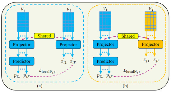
Figure 4.
Base contrastive module. (a) Calculation of frequency band similarity for positive sample pairs. (b) Calculation of frequency band similarity for negative sample pairs.
We extract frequency bands from and a corresponding frequency band from . These extracted frequency bands are then passed through a projector h to obtain the respective feature maps and using the formula
Then, we utilize a predictor to predict the final value and of and accordingly:
| Algorithm 2: Implementation of base contrastive module. |
 |
In Figure 4b, represents the computation of negative cosine similarity between and in the negative sample pair, as expressed by the formula
The notation “stopgrad” indicates that gradient computation is paused, considering as a constant value. Here, represents the norm. Similarly, let denote the negative cosine similarity between and , which can be computed by formula (7).
In reference to [30], we set the loss of frequency band f in negative sample pairs as
2.5. Loss Function
During the fine-tuning phase, the complete loss formula is as follows, where denotes a hyperparameter:
The term in the above equation refers to the cross-entropy loss function employed in Fine-tune1, as illustrated in Figure 2. On the other hand, represents the output loss in Fine-tune2. Specifically, can be expressed as
In the equation above, represents the output loss of the corresponding frequency band f within the base contrastive module and is expressed as
Furthermore, denotes the output loss of the corresponding frequency band f in a positive sample pair, exhibiting similarity to Formula (8).
3. Results
In this section, we assess the performance of the proposed few-shot UATR method using two ship-radiated noise datasets. Firstly, we introduce the two datasets and the experimental setup for the recognition task. Then, we present three data augmentation techniques employed for generating positive and negative sample pairs in the fine-tuning process of Fine-tune2, as depicted in Figure 2. These three methods are also applied in the training of all subsequent models. Next, we verify the effectiveness of the model in UATR by comparing it with some classic UATR methods. Additionally, we compare it with different FSL methods to demonstrate its superiority. Furthermore, we explore the cross-domain capabilities of the model by testing it on different datasets. We also analyze the recognition performance across four different levels of noise situations to evaluate the model’s robustness in noisy environments. Finally, we conduct ablation experiments to analyze the impact of different modules in the model on the final performance.
3.1. Datasets
We conduct a comprehensive evaluation of our model’s classification performance using two open-source datasets: ShipsEar [31] and DeepShip [32]. ShipsEar comprises ship-radiated noise recordings collected along the Atlantic coast of Spain in 2012 and 2013. The dataset includes 90 recordings, consisting of 11 different types of boats and a type of natural background noise. Each category contains one or more recordings, ranging in duration from 15 s to 10 min. We segment the recording of each vessel into 2-second durations, yielding a total of 3796 samples following segmentation. The number of samples for each ship category is shown in Table 1.

Table 1.
Number of samples in each category of ShipsEar after slicing.
Deepship is a dataset comprising recordings obtained from the Georgia Delta Node Strait between the years 2016 and 2018. The dataset consists of 47 h and 4 min of real-world underwater recordings from 265 different vessels belonging to 4 categories. These categories include tankers, tugs, passenger ships, and cargo ships, with the corresponding sample counts being presented in Table 2. Data are recorded for different seasons and sea conditions in real-world marine environments.

Table 2.
Number of samples in each category of DeepShip.
3.2. Data Augmentation
To generate the positive and negative sample pairs , , and shown in Figure 2, we employ three augmentation methods: temporal masking, frequency masking [33], and temporal Gaussian interference. These methods are consistently applied in the training of all subsequent models. In temporal Gaussian interference, Gaussian white noise is randomly introduced to the original ship signal, with the noise standard deviation being randomly selected from the range [0, 0.3] to constrain the intensity of the added Gaussian noise. The results of data augmentation for randomly selected ships are shown in Figure 5.
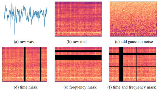
Figure 5.
Diagram with three types of data augmentation.
3.3. Experimental Settings
We conduct five sets of experiments to compare CDCF with classic UATR models and few-shot models. Subsequently, we evaluate its performance in cross-domain scenarios and noisy environments. Furthermore, we conduct ablation experiments to verify the effectiveness of self-supervised training and the base contrastive module.
To ensure consistency, all samples within both datasets are subjected to resampling, resulting in a standardized frequency of 16 kHz. We divide the 11 types of ships in ShipsEar into 2 distinct groups: the base set for pre-training and the novel set for fine-tuning. The base set consists of six ship types, while the novel set comprises five ship types. The categories in the base set are separate from those in the novel set, simulating real-world scenarios where new sample categories may emerge that are not represented in the training set. This division enables us to achieve favorable outcomes by fine-tuning the model on the novel set after pre-training, eliminating the need for retraining. This approach saves computational costs and time. We manually select the categories for the base set and novel set and experiment with three different partitioning methods. A detailed description of each scenario is presented in Table 3.

Table 3.
Categories of base set and novel set in three divisions.
During the fine-tuning phase, ensuring the stability of model results is crucial. We utilize a random selection method, choosing 50 combinations of support set and query set from the novel set. Specifically, for each fine-tuning, distinct samples are employed in the support and query set. The final model result is obtained by averaging all the combination results from the three divisions, as presented in Table 3.
In our experiments, we utilize 128 mel filters to extract mel spectrograms from the input samples as the model input. Specifically, the window length is set to 40 ms, and the frameshift is 20 ms. The loss function initializes the hyperparameter to 1. The AdamW optimizer is utilized for optimization. To evaluate the performance of CDCF, we use accuracy as the primary metric.
3.4. Experimental Results
We train all models using PyTorch on an NVIDIA GeForce RTX 2080 Ti. This section discusses some of the results obtained from the experiments to analyze the performance of the model in cross-domain and noisy environments.
3.4.1. Performance Comparison with State-of-the-Art UATR Models
We conduct experiments on the ShipsEar dataset to validate the effectiveness of FSL methods in UATR, comparing them with traditional methods. Specifically, we compare 1-shot, 3-shot, 5-shot, 10-shot, and 15-shot scenarios for a 5-way classification task. We employ the established UATR model, including ResNet18 [34], CRNN [35], and Transformer (STM) [14], as baseline comparisons. These models have achieved promising results in traditional UATR, and comparing them further highlights the potential of FSL methods. The experimental results are shown in Figure 6.
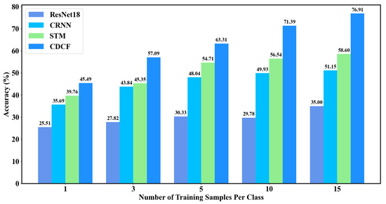
Figure 6.
Performance comparison with state-of-the-art UATR models.
As depicted in Figure 6, CDCF consistently achieves the highest recognition results across all 5-shot situations. With an increasing number of shots for each method, the recognition accuracy continues to improve, and the performance gap between CDCF and the other three traditional UATR methods gradually widens. Particularly, when there are 15 samples per category, CDCF attains an impressive accuracy of 76.91%. Comparing CDCF with the second-best model, CDCF demonstrates improvements of 5.73%, 11.74%, 8.6%, 14.85%, and 18.31% in 1-shot, 3-shot, 5-shot, 10-shot, and 15-shot scenarios, respectively. In contrast, the highest recognition rate achieved by the other three models across all shot situations only reaches 58.60%. Among these three traditional UATR methods, Resnet18 exhibits modest performance improvements as the number of shots increases, while demonstrating notable performance disparities compared to the other two models. When the number of shots increases from one to five for CRNN and STM, their performance experiences rapid enhancement; however, further increases in the number of shots yield minimal performance improvements for both models.
By comparing CDCF with the three traditional UATR methods, it becomes evident that the performance of conventional approaches on few-shot datasets is inadequate. This underscores the necessity of investigating few-shot methods in underwater target recognition scenarios. Concurrently, it validates the effectiveness of FSL in UATR. In practical application scenarios where data are scarce and with high data collection costs, FSL can enhance the model’s ability to generalize from limited samples, enabling it to effectively identify previously unseen categories. To validate the improvement of our approach under few-shot conditions, all subsequent experiments are conducted using the few-shot method.
3.4.2. Performance Comparison of Few-Shot Models
To further evaluate the performance of our model, we conduct a comparative analysis with four other popular few-shot models in the field of image. These models include RelationNet [36], RFS [37], ProtoNet [38], and LabelHallu [39]. Initially, we conduct a few-shot comparative experiment on the ShipsEar dataset. The base set and novel set are divided according to the three methods outlined in Table 3. Consequently, the base set consists of six ship types, while the novel set includes five ship types. The results of a comparison between the few-shot methods on the ShipsEar dataset are presented in Table 4.

Table 4.
Performance comparison of few-shot models on ShipsEar.
We compare the performance of CDCF with four other few-shot models under three scenarios: 1-shot, 3-shot, and 5-shot. In the 1-shot scenario, except for RelationNet, the other four models exhibit similar performance with minimal differences. However, our model consistently achieves optimal results in both the 3-shot and 5-shot scenarios. Specifically, in the 3-shot scenario, CDCF achieves an accuracy of 57.09%, which surpasses the sub-optimal model RFS by 2.02%. Furthermore, in the 5-shot scenario, CDCF’s accuracy further improves compared to the 3-shot scenario, outperforming the sub-optimal model LabelHallu by 3.24%. The observed results illustrate a progressive enhancement in the accuracy of CDCF as the number of shots increases, thereby highlighting its superiority in terms of model performance. These results confirm that CDCF is effective in extracting target features from the novel set in few-shot scenarios, demonstrating the model’s capability to transfer domain knowledge and underscore the potential of employing few-shot models for successful UATR in real-world underwater environments.
3.4.3. Performance Comparison of Few-Shot Models in the Novel Domain
In the experiments presented in Table 4, we perform pre-training and fine-tuning of the model on ShipsEar. In a real marine environment, the characteristics of the marine environmental noise field vary across different sea areas and seasons, leading to some differences in the data collected from different sea areas. To examine the model’s capabilities in cross-domain scenarios, we conduct pre-training on 11 types of ships within the ShipsEar dataset. Subsequently, we perform fine-tuning and evaluate the model’s performance on four types of ships from the DeepShip dataset. To ensure comparability, we employ the same four FSL methods used in Table 4. The experimental results are documented in Table 5.

Table 5.
Performance comparison of few-shot models in the novel domain.
The CDCF demonstrates optimal performance across all three scenarios, including 1-shot, 3-shot, and 5-shot. Notably, it exhibits remarkable improvements over the sub-optimal models, with increases of 4.79%, 5.29%, and 4.84% in accuracy for the 1-shot, 3-shot, and 5-shot cases, respectively. It is worth highlighting that in the challenging 5-shot scenario, CDCF achieves the highest accuracy of 76.93%, showcasing its impressive ability to bridge domain gaps and excel in cross-domain scenarios. The significant performance boost achieved by CDCF further validates its potential in overcoming challenges associated with limited samples learning tasks.
3.4.4. Performance Comparison in Noisy Environments
In UATR, noise interference is an inevitable factor when collecting data. Even the two datasets utilized in our experiments do not consist solely of clean ship-radiated noise; rather, they exhibit a high signal-to-noise ratio (SNR). Evaluating the model’s ability to effectively recognize targets in a noisy environment serves as a measure of its robustness. Hence, we introduce Gaussian white noise with different SNRs to the test data, aiming to assess the model’s anti-noise performance. All models are tested under 5-shot conditions, and the experimental results are illustrated in Figure 7.
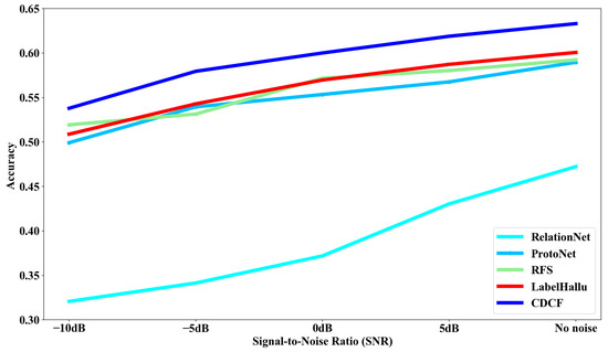
Figure 7.
Performance comparison of few-shot models in noisy environments.
The CDCF demonstrates superior performance compared to the other four models across different SNRs. A notable observation is that among all the models, the RelationNet model demonstrates the lowest performance, whereas the other three models exhibit comparable levels of performance. Even in scenarios with low SNR, CDCF maintains satisfactory recognition capabilities, and its performance steadily improves as the SNR increases. These findings emphasize the robustness of CDCF and its efficacy in effectively mitigating disturbances.
3.4.5. Ablation Experiments
To evaluate the performance improvement in different modules in CDCF, we conduct ablation analysis in 1-shot, 3-shot, and 5-shot scenarios by gradually adding each module to the model. We begin by performing experiments using the traditional FSL method, where the model is pre-trained on the base set, fine-tuned on the support set, and tested on the query set. This approach aligns with the principles outlined in the RFS [37] paper, which we refer to as “TFSL” for clarity and ease of comprehension. To evaluate the influence of self-supervised training on the performance of the model, we incorporate self-supervised training during the fine-tuning process in the traditional FSL framework. This approach is referred to as “CL”. Finally, we further enhance the model by incorporating the base contrastive mudule based on CL, resulting in our proposed CDCF. The ablation results, showcasing the effectiveness of each module, are presented in Table 6.

Table 6.
Experimental results for ablation study.
Ablation experiments validate the effectiveness of the two modules in CDCF. In the 3-shot and 5-shot scenarios, the model’s performance is continuously enhanced as the two modules are incorporated. It is important to note that the 1-shot task represents an extreme scenario, where only one sample per category is available for fine-tuning. The extremely limited amount of data presents challenges for the model to infer meaningful features, resulting in no performance improvement in the 1-shot scenario.
4. Conclusions
This paper presents a novel cross-domain contrastive learning-based few-shot underwater acoustic target recognition method (CDCF) to address the issue of overfitting in few-shot UATR models. CDCF incorporates a self-supervised training branch into traditional FSL to assist with fine-tuning, considering the significant disparity between the source and target domains in underwater scenes. By inputting samples from the target domain and partial samples from the source domain into the self-supervised training branch, the model’s ability to transfer knowledge across domains is enhanced. Additionally, a base contrastive module is introduced to improve the model’s capacity to discriminate spectral information by comparing the similarity of corresponding frequency bands in the feature maps of positive and negative sample pairs. This comparison enables the capture of more fine-grained features, thereby expanding the knowledge scope of the source domain and enhancing the model’s generalization ability.
CDCF is evaluated using two publicly available underwater ship-radiated noise datasets, namely, ShipsEar and DeepShip. The experimental results demonstrate the superior performance of our method in few-shot UATR. Our model achieves optimal performance not only in underwater scenes but also in few-shot cross-domain scenarios, thus confirming its effectiveness and highlighting its capability to transfer domain knowledge in new fields. Furthermore, the robustness of the model in noisy environments is assessed by testing its recognition performance under different SNRs. Overall, CDCF exhibits excellent performance across multiple underwater scenes and shows potential for real-world applications. In future work, we aim to further enhance the model’s performance to meet a wider range of UATR scenarios.
Author Contributions
Conceptualization, X.C., Z.H. and Y.X.; methodology, X.C., Z.H. and Y.X.; software, X.C., Z.H. and Y.X.; validation, X.C., Z.H., Y.X., K.T., P.Z. and J.H.; formal analysis, Z.H. and Y.X.; investigation, Z.H. and Y.X.; resources, X.C. and P.Z.; data curation, Z.H. and Y.X.; writing—original draft preparation, Z.H.; writing—review and editing, X.C., Z.H. and P.Z.; visualization, Z.H.; supervision, X.C. and P.Z.; project administration, X.C. All authors have read and agreed to the published version of the manuscript.
Funding
This project was supported by the National Science Foundation for Young Scientists of China (Grant No.: 62003273) and the Natural Science Basic Research Program of Shaanxi (Program No.: 2020JQ-217).
Institutional Review Board Statement
Not applicable.
Informed Consent Statement
Not applicable.
Data Availability Statement
Data are available in a publicly accessible repository. The data used in this study are openly available at https://underwaternoise.atlanttic.uvigo.es/ (accessed on 29 January 2024) and https://github.com/irfankamboh/DeepShip (accessed on 29 January 2024).
Conflicts of Interest
The authors declare no conflicts of interest.
Abbreviations
The following abbreviations are used in this manuscript:
| UATR | Underwater Acoustic Target Recognition |
| FSL | Few-shot learning |
| STFT | Short-time Fourier transform |
| MFCC | Mel-frequency cepstrum coefficient |
| CDCF | Cross-domain contrastive learning-based few-shot |
| SNR | Signal-to-noise ratio |
References
- Ji, F.; Ni, J.; Li, G.; Liu, L.; Wang, Y. Underwater Acoustic Target Recognition Based on Deep Residual Attention Convolutional Neural Network. J. Mar. Sci. Eng. 2023, 11, 1626. [Google Scholar] [CrossRef]
- Terayama, K.; Shin, K.; Mizuno, K.; Tsuda, K. Integration of sonar and optical camera images using deep neural network for fish monitoring. Aquac. Eng. 2019, 86, 102000. [Google Scholar] [CrossRef]
- Zhang, L.; Wu, D.; Han, X.; Zhu, Z. Feature extraction of underwater target signal using mel frequency cepstrum coefficients based on acoustic vector sensor. J. Sens. 2016, 2016, 7864213. [Google Scholar] [CrossRef]
- Zhu, P.; Zhang, Y.; Huang, Y.; Zhao, C.; Zhao, K.; Zhou, F. Underwater acoustic target recognition based on spectrum component analysis of ship radiated noise. Appl. Acoust. 2023, 211, 109552. [Google Scholar] [CrossRef]
- Azimi-Sadjadi, M.R.; Yao, D.; Huang, Q.; Dobeck, G.J. Underwater target classification using wavelet packets and neural networks. IEEE Trans. Neural Netw. 2000, 11, 784–794. [Google Scholar] [CrossRef] [PubMed]
- Wei, X.; Gang-Hu, L.; Wang, Z. Underwater target recognition based on wavelet packet and principal component analysis. Comput. Simul. 2011, 28, 8–290. [Google Scholar]
- Khishe, M. Drw-ae: A deep recurrent-wavelet autoencoder for underwater target recognition. IEEE J. Ocean. Eng. 2022, 47, 1083–1098. [Google Scholar] [CrossRef]
- Miao, Y.; Zakharov, Y.V.; Sun, H.; Li, J.; Wang, J. Underwater acoustic signal classification based on sparse time—Frequency representation and deep learning. IEEE J. Ocean. Eng. 2021, 46, 952–962. [Google Scholar] [CrossRef]
- Miao, Y.; Li, J.; Sun, H. Multimodal Sparse Time—Frequency Representation for Underwater Acoustic Signals. IEEE J. Ocean. Eng. 2020, 46, 642–653. [Google Scholar] [CrossRef]
- Doan, V.S.; Huynh-The, T.; Kim, D.S. Underwater acoustic target classification based on dense convolutional neural network. IEEE Geosci. Remote Sens. Lett. 2020, 19, 1–5. [Google Scholar] [CrossRef]
- Hong, F.; Liu, C.; Guo, L.; Chen, F.; Feng, H. Underwater acoustic target recognition with a residual network and the optimized feature extraction method. Appl. Sci. 2021, 11, 1442. [Google Scholar] [CrossRef]
- Yang, S.; Xue, L.; Hong, X.; Zeng, X. A Lightweight Network Model Based on an Attention Mechanism for Ship-Radiated Noise Classification. J. Mar. Sci. Eng. 2023, 11, 432. [Google Scholar] [CrossRef]
- Jin, A.; Zeng, X. A Novel Deep Learning Method for Underwater Target Recognition Based on Res-Dense Convolutional Neural Network with Attention Mechanism. J. Mar. Sci. Eng. 2023, 11, 69. [Google Scholar] [CrossRef]
- Li, P.; Wu, J.; Wang, Y.; Lan, Q.; Xiao, W. STM: Spectrogram Transformer Model for Underwater Acoustic Target Recognition. J. Mar. Sci. Eng. 2022, 10, 1428. [Google Scholar] [CrossRef]
- Zhang, M.; Luo, X. Underwater Acoustic Target Recognition Based on Generative Adversarial Network Data Augmentation. In Proceedings of the INTER-NOISE and NOISE-CON Congress and Conference Proceedings, Washington, DC, USA, 1–4 August 2021; Institute of Noise Control Engineering: Washington, DC, USA, 2021; Volume 263, pp. 4558–4564. [Google Scholar]
- Luo, X.; Zhang, M.; Liu, T.; Huang, M.; Xu, X. An underwater acoustic target recognition method based on spectrograms with different resolutions. J. Mar. Sci. Eng. 2021, 9, 1246. [Google Scholar] [CrossRef]
- Radford, A.; Metz, L.; Chintala, S. Unsupervised representation learning with deep convolutional generative adversarial networks. arXiv 2015, arXiv:1511.06434. [Google Scholar]
- Huang, G.; Liu, Z.; Van Der Maaten, L.; Weinberger, K.Q. Densely connected convolutional networks. In Proceedings of the IEEE Conference on Computer Vision and Pattern Recognition, Honolulu, HI, USA, 21–26 July 2017; pp. 4700–4708. [Google Scholar]
- Gao, Y.; Chen, Y.; Wang, F.; He, Y. Recognition method for underwater acoustic target based on DCGAN and DenseNet. In Proceedings of the 2020 IEEE 5th International Conference on Image, Vision and Computing (ICIVC), Beijing, China, 10–12 July 2020; pp. 215–221. [Google Scholar]
- Wang, Y.; Anderson, D.V. Hybrid attention-based prototypical networks for few-shot sound classification. In Proceedings of the ICASSP 2022—2022 IEEE International Conference on Acoustics, Speech and Signal Processing (ICASSP), Singapore, 22–27 May 2022; pp. 651–655. [Google Scholar]
- Wang, Y.; Stoller, D.; Bittner, R.M.; Bello, J.P. Few-shot musical source separation. In Proceedings of the ICASSP 2022—2022 IEEE International Conference on Acoustics, Speech and Signal Processing (ICASSP), Singapore, 22–27 May 2022; pp. 121–125. [Google Scholar]
- You, L.; Coyotl, E.P.; Gunturu, S.; Van Segbroeck, M. Transformer-Based Bioacoustic Sound Event Detection on Few-Shot Learning Tasks. In Proceedings of the ICASSP 2023-2023 IEEE International Conference on Acoustics, Speech and Signal Processing (ICASSP), Rhodes Island, Greece, 4–10 June 2023; pp. 1–5. [Google Scholar]
- Chen, Y.; Ma, Q.; Yu, J.; Chen, T. Underwater acoustic object discrimination for few-shot learning. In Proceedings of the 2019 4th International Conference on Mechanical, Control and Computer Engineering (ICMCCE), Hohhot, China, 24–26 October 2019; pp. 430–4304. [Google Scholar]
- Xue, L.; Zeng, X.; Yan, X.; Yang, S. Completion-Attention Ladder Network for Few-Shot Underwater Acoustic Recognition. Neural Process. Lett. 2023, 55, 9563–9579. [Google Scholar]
- Chungath, T.T.; Nambiar, A.M.; Mittal, A. Transfer Learning and Few-Shot Learning Based Deep Neural Network Models for Underwater Sonar Image Classification with a Few Samples. IEEE J. Ocean. Eng. 2023, 1–17. [Google Scholar] [CrossRef]
- Nie, L.; Li, C.; Wang, H.; Wang, J.; Zhang, Y.; Yin, F.; Marzani, F.; Bozorg Grayeli, A. A Contrastive-Learning-Based Method for the Few-Shot Identification of Ship-Radiated Noises. J. Mar. Sci. Eng. 2023, 11, 782. [Google Scholar] [CrossRef]
- Tian, S.; Bai, D.; Zhou, J.; Fu, Y.; Chen, D. Few-shot learning for joint model in underwater acoustic target recognition. Sci. Rep. 2023, 13, 17502. [Google Scholar] [CrossRef] [PubMed]
- Jaiswal, A.; Babu, A.R.; Zadeh, M.Z.; Banerjee, D.; Makedon, F. A survey on contrastive self-supervised learning. Technologies 2020, 9, 2. [Google Scholar] [CrossRef]
- Hua, J.; Cui, X.; Li, X.; Tang, K.; Zhu, P. Multimodal fake news detection through data augmentation-based contrastive learning. Appl. Soft Comput. 2023, 136, 110125. [Google Scholar] [CrossRef]
- Chen, X.; He, K. Exploring simple siamese representation learning. In Proceedings of the IEEE/CVF Conference on Computer Vision and Pattern Recognition, Nashville, TN, USA, 20–25 June 2021; pp. 15750–15758. [Google Scholar]
- Santos-Domínguez, D.; Torres-Guijarro, S.; Cardenal-López, A.; Pena-Gimenez, A. ShipsEar: An underwater vessel noise database. Appl. Acoust. 2016, 113, 64–69. [Google Scholar] [CrossRef]
- Irfan, M.; Jiangbin, Z.; Ali, S.; Iqbal, M.; Masood, Z.; Hamid, U. DeepShip: An underwater acoustic benchmark dataset and a separable convolution based autoencoder for classification. Expert Syst. Appl. 2021, 183, 115270. [Google Scholar] [CrossRef]
- Park, D.S.; Chan, W.; Zhang, Y.; Chiu, C.C.; Zoph, B.; Cubuk, E.D.; Le, Q.V. Specaugment: A simple data augmentation method for automatic speech recognition. arXiv 2019, arXiv:1904.08779. [Google Scholar]
- Hong, F.; Liu, C.; Guo, L.; Chen, F.; Feng, H. Underwater acoustic target recognition with resnet18 on shipsear dataset. In Proceedings of the 2021 IEEE 4th International Conference on Electronics Technology (ICET), Chengdu, China, 7–10 May 2021; pp. 1240–1244. [Google Scholar]
- Liu, F.; Shen, T.; Luo, Z.; Zhao, D.; Guo, S. Underwater target recognition using convolutional recurrent neural networks with 3-D Mel-spectrogram and data augmentation. Appl. Acoust. 2021, 178, 107989. [Google Scholar] [CrossRef]
- Sung, F.; Yang, Y.; Zhang, L.; Xiang, T.; Torr, P.H.; Hospedales, T.M. Learning to compare: Relation network for few-shot learning. In Proceedings of the IEEE Conference on Computer Vision and Pattern Recognition, Salt Lake City, UT, USA, 18–23 June 2018; pp. 1199–1208. [Google Scholar]
- Tian, Y.; Wang, Y.; Krishnan, D.; Tenenbaum, J.B.; Isola, P. Rethinking few-shot image classification: A good embedding is all you need? In Proceedings of the Computer Vision—ECCV 2020: 16th European Conference, Glasgow, UK, 23–28 August 2020; Proceedings, Part XIV 16. Springer: Cham, Switzerland, 2020; pp. 266–282. [Google Scholar]
- Snell, J.; Swersky, K.; Zemel, R. Prototypical networks for few-shot learning. Adv. Neural Inf. Process. Syst. 2017, 30, 4077–4087. [Google Scholar]
- Jian, Y.; Torresani, L. Label hallucination for few-shot classification. In Proceedings of the AAAI Conference on Artificial Intelligence, Online, 22 February–1 March 2022; Volume 36, pp. 7005–7014. [Google Scholar]
Disclaimer/Publisher’s Note: The statements, opinions and data contained in all publications are solely those of the individual author(s) and contributor(s) and not of MDPI and/or the editor(s). MDPI and/or the editor(s) disclaim responsibility for any injury to people or property resulting from any ideas, methods, instructions or products referred to in the content. |
© 2024 by the authors. Licensee MDPI, Basel, Switzerland. This article is an open access article distributed under the terms and conditions of the Creative Commons Attribution (CC BY) license (https://creativecommons.org/licenses/by/4.0/).