Numerical Simulation of Seakeeping Performance of a Barge Using Computational Fluid Dynamics (CFD)-Modified Potential (CMP) Model

Abstract

This paper explains the evaluation process of seakeeping performance for small vessels using a CFD-modified potential (CMP) model, a hybrid simulation model that modifies the damping ratio with computational fluid dynamics (CFD) after analyzing ship motion based on the linear potential theory. From the result of the motion analysis using the CMP model, the seakeeping performance of a small vessel (a barge here) was evaluated on the basis of the single significant amplitude (SSA) under the sea states 2~4. The results of the motion RAOs and seakeeping performance evaluation were verified through comparison with the results obtained by performing model tests and potential flow programs only. In all sea states, the relative errors (compared to the experiment) of roll motion using the CMP model were relatively small compared to the results using the potential flow program and tended to decrease more as the sea state increased. On the other hand, the results of pitch motion using the CMP model were underestimated in all sea states compared to the experiment. However, it is seen that they are relatively closer to the experiment compared to the results using a potential flow program only.

1. Introduction

Numerical simulations have become increasingly important in evaluating the seakeeping performance of both conventional and high-speed vessels, particularly as a valuable tool in ship design. Small vessels experience relatively large motions in marine environments compared to larger ships, which puts them at a greater risk of stability issues [1]. Therefore, conducting seakeeping analysis during the design stage is crucial. The motion analysis of small vessels requires considering not only the roll motion but also pitch and other motions that significantly affect stability. Consequently, studies on the six-degree-of-freedom (DOF) motion and seakeeping performance of small vessels primarily rely on a potential program in the frequency domain, allowing for efficient calculations. For instance, Prini et al. [2] investigated the heave and pitch motions of a search and rescue (SAR) craft in regular waves using linear potential theory, while Sclavounos and Borgen [3] employed a three-dimensional Rankine panel method based on linear potential theory to study the seakeeping performance of a foil-assisted high-speed monohull vessel. Lewandowski [4] calculated the wave-induced motion of two vessels in close proximity using linear potential theory. Zhang et al. [5] studied three-dimensional, time-domain, ship–wave interactions for problems with forward speed using potential theory. However, small vessels are subject to nonlinearity of damping effects caused by fluid viscosity, making it crucial to accurately estimate damping coefficients for predicting their hull stability and seakeeping performance. The commonly used linear potential theory has limitations in accurately predicting strong nonlinear viscous effects and determining suitable damping coefficients for ship motion analysis [6].

To address these limitations, computational fluid dynamics (CFD) simulations have been used in several studies. For example, Toxopeus et al. [7] conducted a validation study using various computational models, including a low-fidelity system-based model, potential model, and high-fidelity CFD, to solve ship hydrodynamics. Their findings indicated that high-fidelity CFD is necessary to accurately capture all the relevant physics during wave operations. Similarly, Niklas and Pruszko [8] employed comprehensive CFD simulations to evaluate seakeeping performance, validating the results against experimental testing in a towing tank. Moreover, Simonsen et al. [9] performed CFD simulations to predict the heave and pitch motion of the KRISO Container Ship (KCS) model, demonstrating good agreement with experimental results obtained in the towing tank. These examples highlight the consistent agreement between CFD studies and experimental data. Additionally, Im and Lee [10] evaluated the effects of wave height and forward speed on the seakeeping performance of a small fishing vessel in irregular waves using CFD. Ozturk et al. [11] studied the full-scale resistance and seakeeping performance of an awarded Double-M craft designed as a 15 m Emergency Response and Rescue Vessel (ERRV). Fitriadhy et al. [12] presents CFD analysis on the seakeeping performance of a training ship quantified through Response of Amplitude Operators (RAOs) for heave and pitch motions. However, CFD simulations require extensive simulations across various frequencies and wave directions, which can be computationally costly for seakeeping performance analysis. To overcome this limitation, Kim et al. [13] proposed a hybrid simulation model that utilizes CFD to calibrate the damping ratio at the peak point of the ship response spectrum, as analyzed by a potential-based model for seakeeping analysis. Nevertheless, challenges remain, such as the ambiguity in calculating the damping ratio when a double peak appears in the ship response spectrum and the need for further verification of the analysis results to ensure their reliability.

To address these concerns, Nam et al. [14] proposed a simulation procedure that modifies the model introduced by Kim et al. [13], resulting in the “CFD-Modified Potential (CMP) model”. Unlike the hybrid simulation model proposed by Kim et al. [13], the CMP model applied the damping ratio correction via the CFD result at the maximum peak frequency of the motion RAO, rather than on the ship response spectrum. This modification leads to a more accurate damping ratio, even when experimental data are unavailable. However, it is important to note that Nam et al. [14] applied this model exclusively to a barge operating under only sea state 2, which is considered one of the lowest sea conditions according to the Word Meteorological Organization (WMO) sea state classification standard [15]. For small ships, as their stability is significantly influenced by the marine environment, it is crucial to validate the CMP model under more severe conditions (i.e., sea states 3, 4, and beyond) to comprehensively assess their seakeeping performance. Additionally, Sariöz, and Narli [16] emphasized the importance of evaluating seakeeping performance for each combination of wave heading and sea states.

The main goal of this study was to evaluate the applicability and effectiveness of the CMP model in analyzing seakeeping performance of a barge under a wide spectrum of sea conditions. The analysis specifically targeted sea states 3 and 4, recognized for their higher wave heights as defined by the WMO sea state codes. For the seakeeping analyses, motion RAOs were predicted utilizing both potential flow programs and CFD simulations in a computational framework of the CMP model. To verify the accuracy and reliability of the CMP model, the results of the RAOs were compared with experimental data. This investigation helps to ascertain the CMP model’s suitability for evaluating the seakeeping performance of a barge across diverse and challenging marine environments. This encompasses both the moderate and rough conditions of sea states 3 and 4, as well as the calmer scenarios represented by sea state 2.

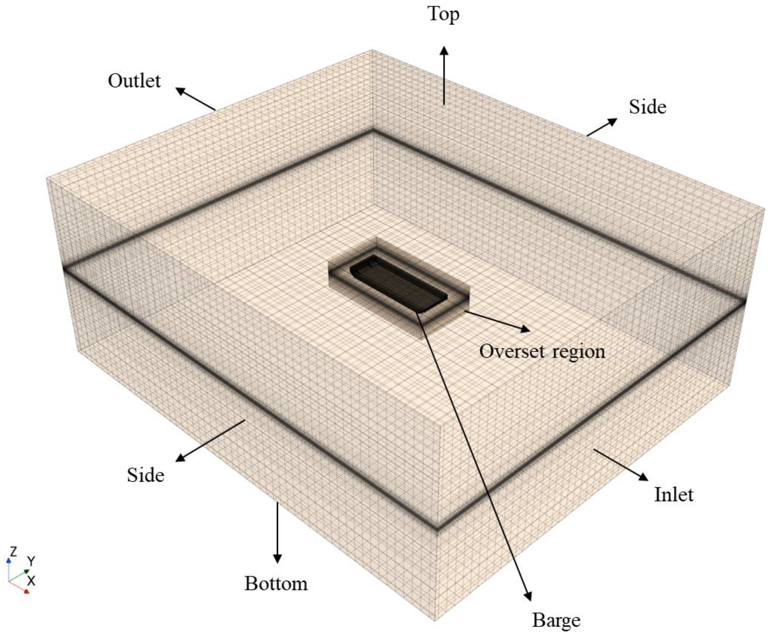
2. Simulation Modeling

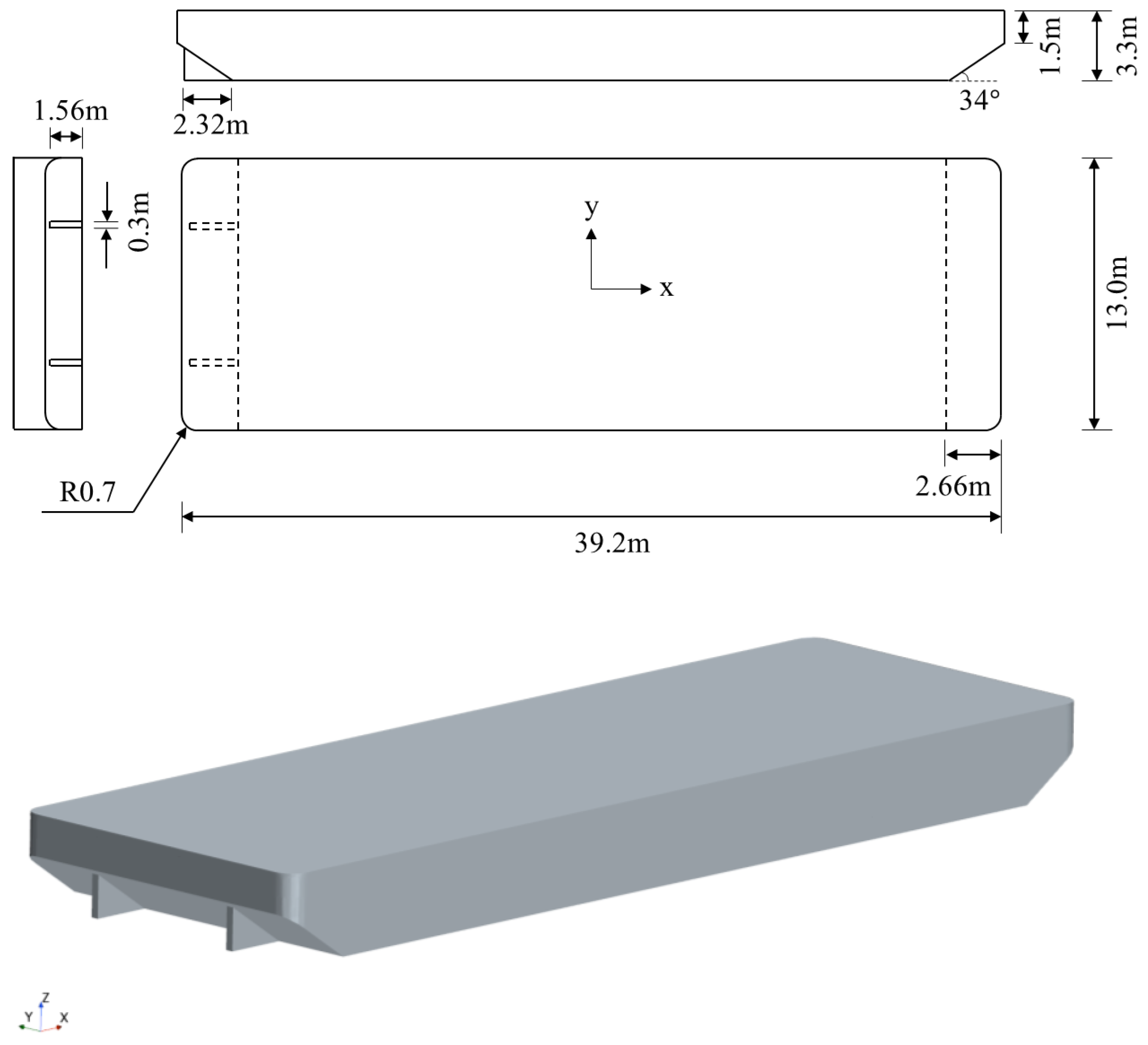
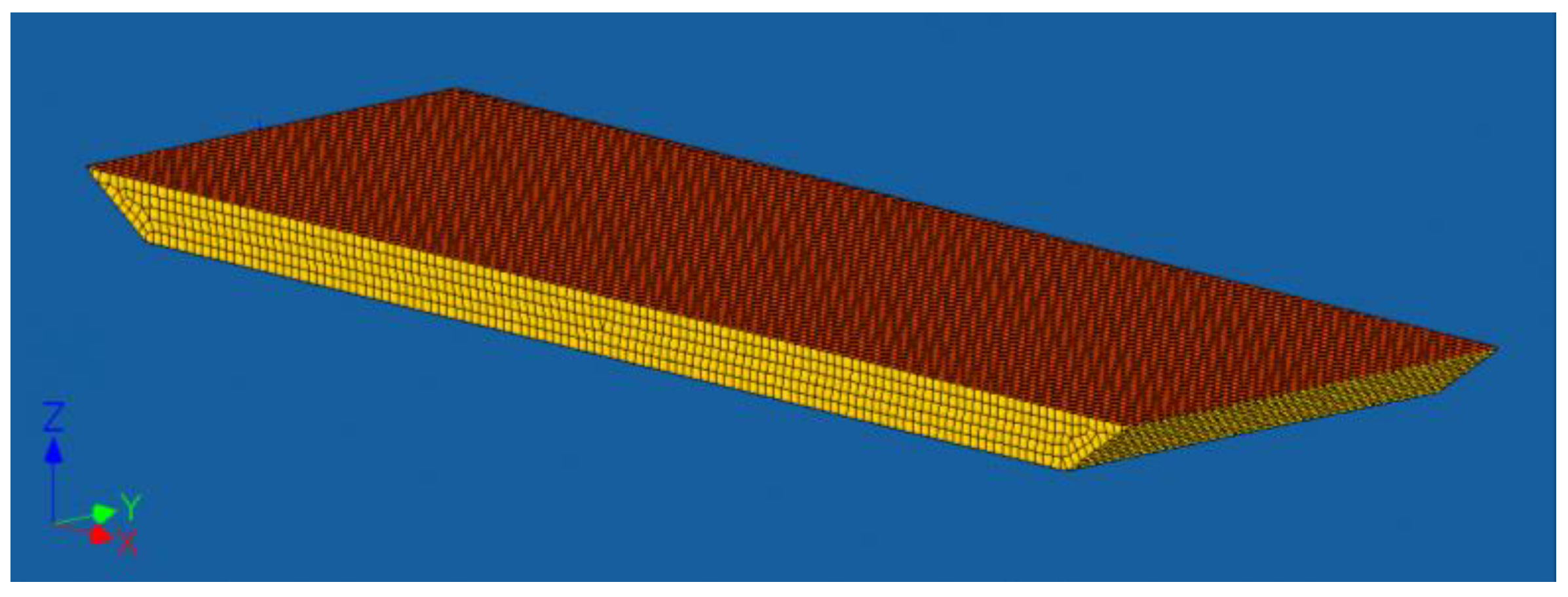
2.1. Target Model

The model selected for this study was a barge as depicted in Figure 1. The full-scale dimensions of the barge are provided in

Table 1. Principal dimensions of barge.

Principal Dimension	Full-Scale
Length between perpendicular, Lpp (m)	39.2
Breadth, B (m)	13.0
Depth, D (m)	3.3
Draft, T (m)	1.5
Displacement weight, W (kgf)	735,000
Longitudinal center of gravity, LCG from AP (m)	19.6
Vertical center of gravity, VCG from BL (m)	2.7
Moment of inertia, Ixx (kg·m2)	9,055,273
Moment of inertia, Iyy and Izz (kg·m2)	70,589,400
Speed, U (m·s−1)	3.0

. It measured 39.2 m in length. The barge exhibited a flat bottom and was symmetrical both from side to side and fore and aft, with two skegs installed at the stern. The velocity of the barge was set to 3.0 m·s⁻¹, which corresponds to its design speed. All simulations obtaining RAOs were performed using a model at a 1/39.2 scale to ensure fidelity to the experimental setup and to minimize scaling discrepancies.

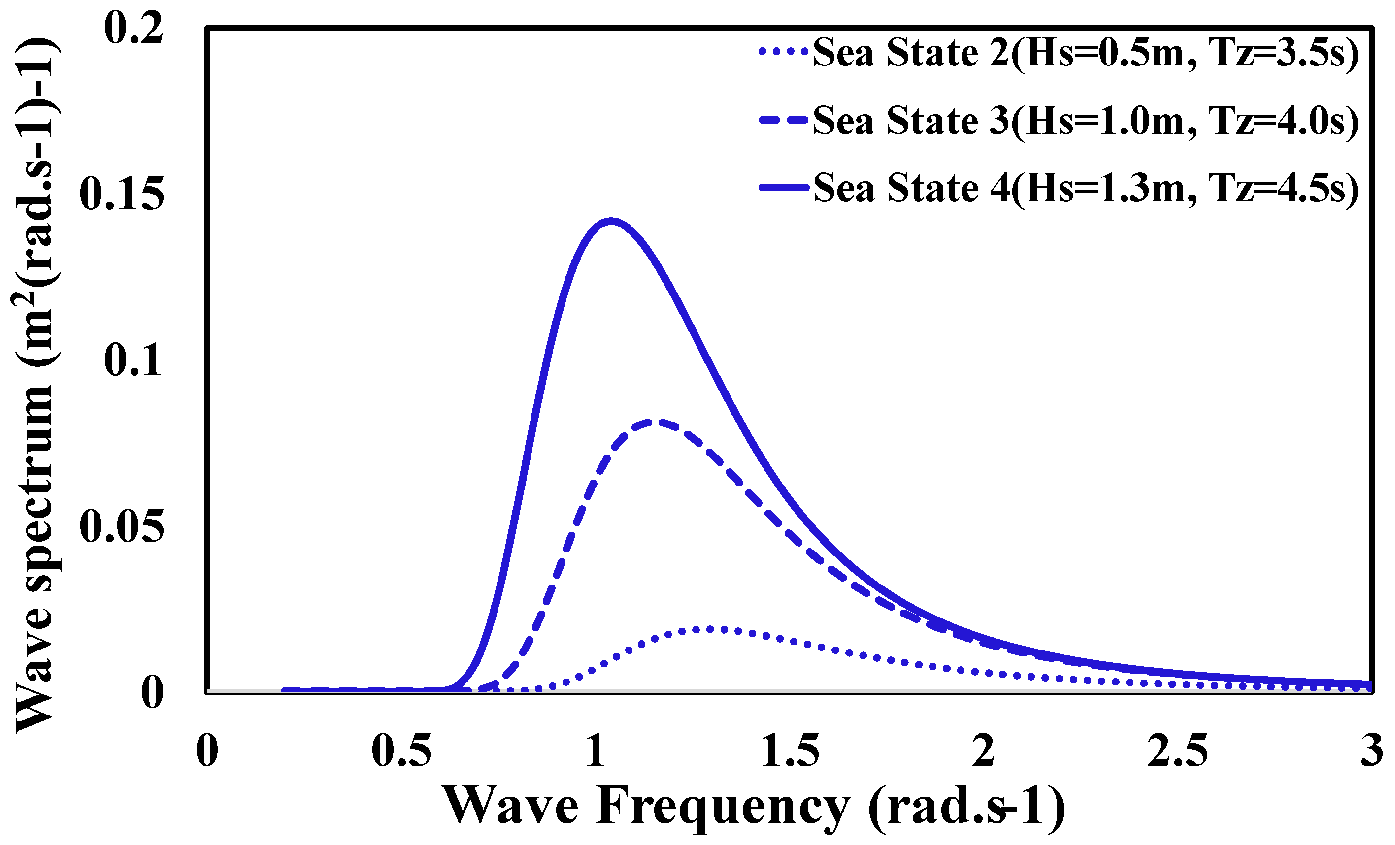
2.2. Sea Environmental Conditions and Wave Spectrum

The Shinan sea area, located in the southwest sea of Korea (34.73 N, 126.24 E), was selected as the target area for barge operation. Wave data comprising approximately 30,000 observations were collected over the past five years, providing information on the wave height and average zero-crossing wave period within the target sea [17]. These data were categorized based on the sea state code classification criteria established by the WMO. Significant wave height was classified at 0.1 m intervals, while the average zero-crossing wave period was classified at 0.5 s intervals. Seakeeping performance evaluation typically occurs under higher sea states, including extreme conditions. Therefore, this study focused on analyzing the barge’s seakeeping performance under the most critical conditions at the target sea site, aiming to demonstrate the applicability of the CMP model across various sea states. Consequently, the significant wave height and average zero-crossing wave period with the highest wave energy among those generated in each sea state were selected.

Table 2. Conditions of wave height and zero-crossing wave period.

Sea State Code	Hs (m)	Tz (s)
Sea State 2	0.5	3.5
Sea State 3	1.0	4.0
Sea State 4	1.3	4.5

presents the final conditions chosen for each sea state 2, 3, and 4.

For the selection of the wave spectrum, Suh et al. [18], who statistically analyzed examples of the wave spectrum suitable for the wave height and wave period conditions along the coast of Korea, were referred to. The TMA (Texel–Marsen–Arsloe) spectrum [19] was selected as the wave spectrum to be used in this study. The TMA spectrum incorporates the influence of a finite water depth by multiplying the shape function developed by Kitaigordskii et al. [20] with the JONSWAP spectrum. The JONSWAP spectrum was determined using the formula proposed by Goda [21], while Kitaigordskii’s shape function was approximated using the formulation proposed by Thompson and Vincent [22]. Equation (1) represents the formula for the TMA spectrum. The Phillips parameter $\mathsf{\alpha }$, which depends on the peak enhancement factor γ, can be calculated using Equation (2). As per DNV-OS-E301 [23], $\gamma$ can be defined using Equation (3), and we used a value of 1 for $\gamma$ in this particular sea area based on the formula. Moreover, $\omega$ represents the wave frequency and ${\omega }_p$ denotes the peak frequency. A variable parameter $\mathsf{\sigma }$ is defined based on the relationship between $\omega$ and ${\omega }_p$, as given in Equation (4). The transformation factor $\phi \left({\omega }_h\right)$ indicates the effect of the water depth $h$, and it can be determined by Equation (5). Here, ${\omega }_h$ can be derived by Equation (6), where $g$ is gravitational acceleration. The spectral peak period $T_P$ is estimated by Equation (7). Figure 2 illustrates the TMA spectrum of the Shinan sea calculated using these formulas.

$$\mathrm{S}\left(\omega \right)=\frac{\alpha H_s^2{\omega }_p^4}{\omega }\mathrm{e}\mathrm{x}\mathrm{p}\left[-1.25{\left(\frac{{\omega }_p}{\omega }\right)}^4\right]{\gamma }^{exp\left[-\frac{{(\omega -{\omega }_p)}^2}{2{\sigma }^2{\omega }_p^2}\right]}\phi \left({\omega }_h\right)$$

(1)

$$\mathsf{\alpha }=\frac{0.0624(1.094-0.01915\ln \gamma )}{0.23+0.0336\gamma -\frac{0.185}{1.9+\gamma }}$$

(2)

$$\gamma =\left\{\begin{array}{c}5,if(\frac{T_p}{\sqrt{H_s}}\le 3.6)\\ e^{5.75-1.15\frac{T_p}{\sqrt{H_s}}},if(3.6\le \frac{T_p}{\sqrt{H_s}}\le 5)\\ 1,if(5\le \frac{T_p}{\sqrt{H_s}})\end{array}\right.$$

(3)

$$\mathsf{\sigma }=\left\{\begin{array}{c}0.07,if(\omega \le {\omega }_p)\\ 0.09,if(\omega >{\omega }_p)\end{array}\right.$$

(4)

$$\phi \left({\omega }_h\right)=\left\{\begin{array}{c}0.5{\omega }_h^2,if({\omega }_h\le 1)\\ 1-0.5{\left(2-{\omega }_h\right)}^2,if(1<{\omega }_h\le 2)\\ 1,if({\omega }_h>2)\end{array}\right.$$

(5)

$${\omega }_h=\omega \sqrt{\frac{h}{g}}$$

(6)

$$T_P=\frac{T_z}{\sqrt{\frac{5+\gamma }{10.89+\gamma }}}$$

(7)

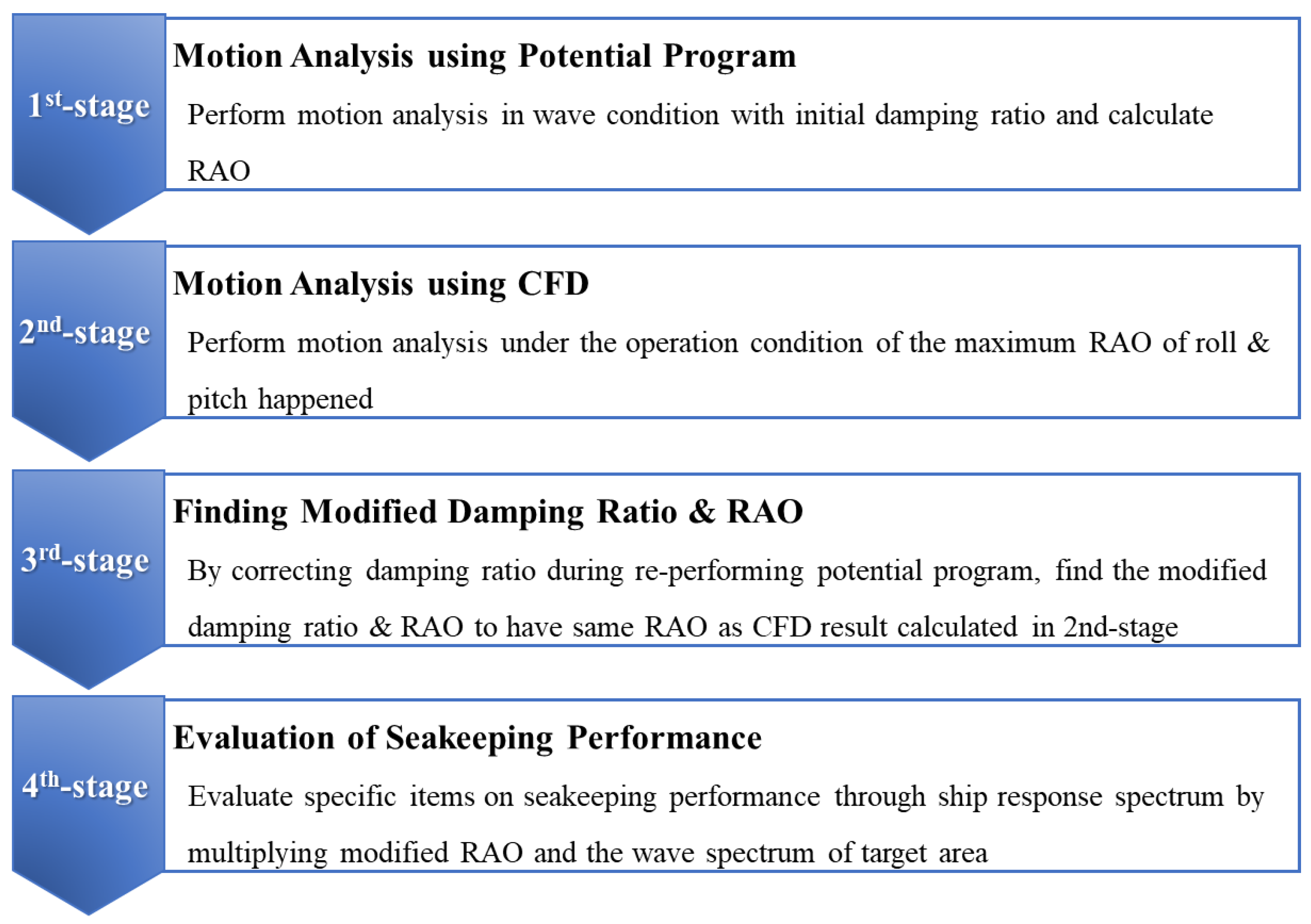
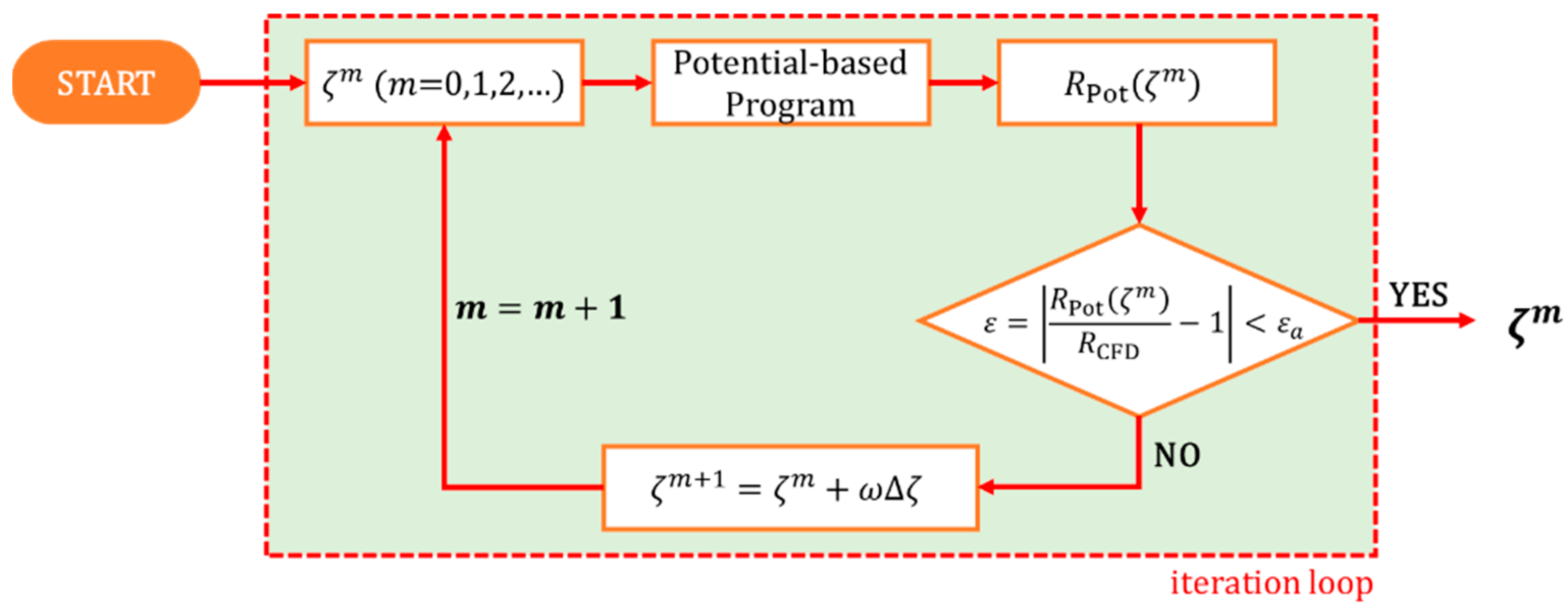
2.3. Simulation Procedure of CMP Model

In this study, numerical simulations were conducted to evaluate the motion and seakeeping performances of the barge under the given wave conditions, following the computational procedure of the CMP model as outlined in Figure 3. Please refer to [14] for detailed information on the procedure. Following each procedure, the simulation execution is briefly summarized in Figure 3.

• [First stage] Motion analysis using potential flow program

In the first stage of the CMP model, the hull motion RAO is calculated under zero-speed conditions using a potential flow program. In this study, WAVELOAD-FD, which is the potential flow program at Lloyd’s Register [24], was used. As shown in Figure 4, approximately 30,000 subsurface mesh cells were generated for the analysis. The directions were set at 30° intervals from 180° to 0°, and the frequency was set at 0.05 rad·s⁻¹ intervals from 0.2 rad·s⁻¹ to 3.0 rad·s⁻¹ based on the ABS Guidance Notes (2003) [25]. The water depth was set as 20 m, which is the average water depth in the target sea area. A specific roll damping ratio is required to perform hull motion analysis using a potential flow program. Typically, this damping ratio is determined by calculations derived from a free decay test, conducted either experimentally or through CFD. The first stage of the CMP model aims to obtain information about the frequency and wave direction where the maximum peak of the roll RAO occurs, and that information is generally not affected by the damping ratio. In the analysis process of the CMP model, the initial damping ratio applied at the first stage will be corrected in the subsequent third stage. For this study, the initial roll damping ratio was assumed to be 0.10, a commonly used value. Conversely, the initial pitch damping ratio was set to 0.

• [Second stage] Motion analysis using CFD

In the second stage, hull motion analysis through CFD is performed under a specific wave period and the wave direction conditions where the maximum value of RAO calculated in the previous step occurs. The motion of viscous fluid can be described with continuity and Navier–Stokes equations. They are derived from the law of conservation of momentum and by the introduction of constitutive equations. Constitutive equations divide stress in the fluid on the viscous and pressure terms [26]. The equations of continuity and Reynolds-averaged Navier–Stokes (RaNS) for incompressible and viscous fluid are given by Equations (8) and (9), respectively:

$$\frac{{\partial u}_i}{{\partial x}_j}=0$$

(8)

$$\frac{\partial }{\partial t}\left(\rho {\overline{u}}_i\right)+\frac{\partial }{{\partial x}_j}\left(\rho {\overline{u}}_i{\overline{u}}_j\right)=-\frac{\partial \overline{p}}{{\partial x}_i}+\frac{\partial }{{\partial x}_j}\left[\mu \left(\frac{\partial {\overline{u}}_i}{{\partial x}_j}+\frac{\partial {\overline{u}}_j}{{\partial x}_i}\right)-\rho \overline{u_i^{\prime }{u}_j^{\prime }}\right]$$

(9)

where, $\rho$ is the density, $\overline{u}$ is the mean velocity, $t$ is the time, $x$ is the coordinate, $\overline{p}$ is the mean pressure, $\mu$ is the dynamic viscosity, and $\overline{u_i^{\prime }{u}_j^{\prime }}$ is the Reynolds stress.

For the RaNS-based simulation, STAR-CCM+15.02 (Siemens PLM Software, Plano, TX, USA) was used in this study. The domain of a numerical tank for simulation is shown in Figure 5. Here, ship speed (design speed or target ship speed) must be considered for hull motion analysis using CFD. This is because the motion of an operating vessel is distinctly different from that of a vessel without forward speed. In addition, hull motion analysis through CFD is performed under conditions where maximum values occur in both RAOs of roll and pitch. This is because the roll motion is the most dominant value in the case of large ships, but in the case of small ships, excessive motion occurs not only in roll motion but also in pitch motion, which greatly affects stability and safety.

In the case of the mesh model, an overset mesh that can better control the local mesh characteristics when the geometry moves through the domain is used for the motion analysis of a ship with a lot of relative movement, which was selected for this study. Furthermore, a surface remesher and trimmed cell mesher were used for grid generation. To accurately capture the effects of fluid viscosity near the moving hull, a prism layer mesher was employed. A total of eight prism layers were applied around the hull to achieve a y+ value of 4 or less, utilizing a low y+ wall treatment to effectively resolve the viscous sublayer. As highlighted by [27], the mesh quality in the vicinity of the water–air interface significantly influences the precision of wave simulations in multiphase flows, suggesting that achieving satisfactory accuracy typically requires about 80 cells per wavelength and 15~25 cells per wave height. In alignment with these recommendations, the present CFD simulation was configured with approximately 65 cells per wavelength and 22 grids per wave height. Figure 6 provides a detailed view of the mesh configuration at this stage. For the simulation solvers, a second-order implicit unsteady solver for time and a second-order upwind/central scheme solver for space were used by referring to [28]. The Shear Stress Transport (SST) k − ω model was used for the turbulence model. The time step was adaptively adjusted to maintain the Courant–Friedrichs–Lewy (CFL) condition with a value less than 1.0 throughout the simulation process. The time histories of the roll and pitch RAOs were derived from the time-averaged responses after the transient range through simulation, referring to [29]. The boundary surface configuration of the finest mesh used is depicted in Figure 7, with the specific boundary conditions outlined in

Table 3. Boundary conditions.

Boundary	Condition Setting
Inlet, Top, Bottom	Velocity inlet
Outlet, Side	Pressure outlet
Overset region	Overset

.

At this stage, it is essential to verify the accuracy of the CFD simulation. Therefore, the Grid Convergence Index (GCI) must be calculated by performing a grid convergence test. The GCI theory uses the Richardson Extrapolation method according to the density of the grid, which is based on Taylor expansion as a method of obtaining a higher-order estimate of the continuum value from the discretization value [30,31]. In this simulation, a grid convergence test was conducted using five different grid sizes, as detailed in

Table 4. RAO results from grid convergence tests.

Grid Case	1	2	3	4	5
Grid Base Size	0.35	0.27	0.20	0.15	0.11
No. of Mesh	1,000,000	1,600,000	3,200,000	6,600,000	14,000,000
RAO	10.37	9.97	9.65	9.52	9.51

. The base sizes for each case were determined based on the methodologies described in references [30,31], with a refinement factor of 1.33. Utilizing the RAO results from these tests, four sets of mesh levels—(1, 2, 3), (2, 3, 4), (3, 4, 5), and (1, 3, 5)—were established to calculate the GCI. In Figure 8, the black symbols denote the RAO results for each grid case. The yellow circles represent the mesh level (1, 2, 3), orange diamonds represent the mesh level (2, 3, 4), red triangles represent the mesh level (3, 4, 5), and green stars correspond to the high-order estimates for the mesh level (1, 3, 5). The GCI values showed convergence at the mesh level (3, 4, 5). Consequently, the CFD simulations were performed using a grid comprising 6.6 million cells, corresponding to Grid Case 4.

• [Third stage] Finding modified damping ratio and RAO

The third stage involves determining the damping ratio to be adjusted. In order to determine the modified damping ratio, motion analysis is iteratively performed by adjusting the damping ratio applied to the potential flow program until the peak value of the RAOs matches the calculated results from the CFD in the second stage. The procedure for calculating the modified damping ratio, as suggested by Nam et al. [14], is illustrated in Figure 9. Here, the modified damping ratio (${\zeta }^m$) has a different value compared to the initial damping ratio used in the first stage. Furthermore, the final RAOs obtained in this stage differ from the initial RAOs in the first stage, as potential flow analysis is conducted under the operating condition of the barge.

• [Fourth stage] Evaluation of seakeeping performance

In the fourth stage, the seakeeping performance is evaluated based on the results of the final hull motion analysis. Firstly, the ship response spectrum is derived by multiplying the square of the final RAOs by the wave spectrum of the target sea, as described in Equation (10). In this equation, $S_{\alpha }\left(\omega \right)$ denotes the ship response spectrum, $S_{\omega }\left(\omega \right)$ is the wave spectrum, and $\omega$ is the wave frequency. To quantitatively evaluate the seakeeping performance, it is converted into the significant single amplitude (SSA) evaluation unit using Equation (11). The 0th moment of the response spectrum, denoted as $m_0$, is defined in Equation (12). For the specific evaluation of seakeeping performance in this study, roll and pitch were chosen as the criteria, which were determined by referring to the standards of NORDFORSK [32] and NATO [33] as shown in

Table 5. Evaluation of seakeeping performance criteria.

Motion Response	Reference Location	Units	Criterion
Roll	COG	SSA (deg)	8.0
Pitch	COG	SSA (deg)	3.0

.

$$S_{\alpha }(\omega )=S_{\omega }(\omega )\times {\left|RAO(\omega )\right|}^2$$

(10)

$$SSA=2\sqrt{m_0}$$

(11)

$$m_n={\int }_0^{\infty }{\omega }_e^n{S}_{\alpha }\left(\omega \right)\delta \omega$$

(12)

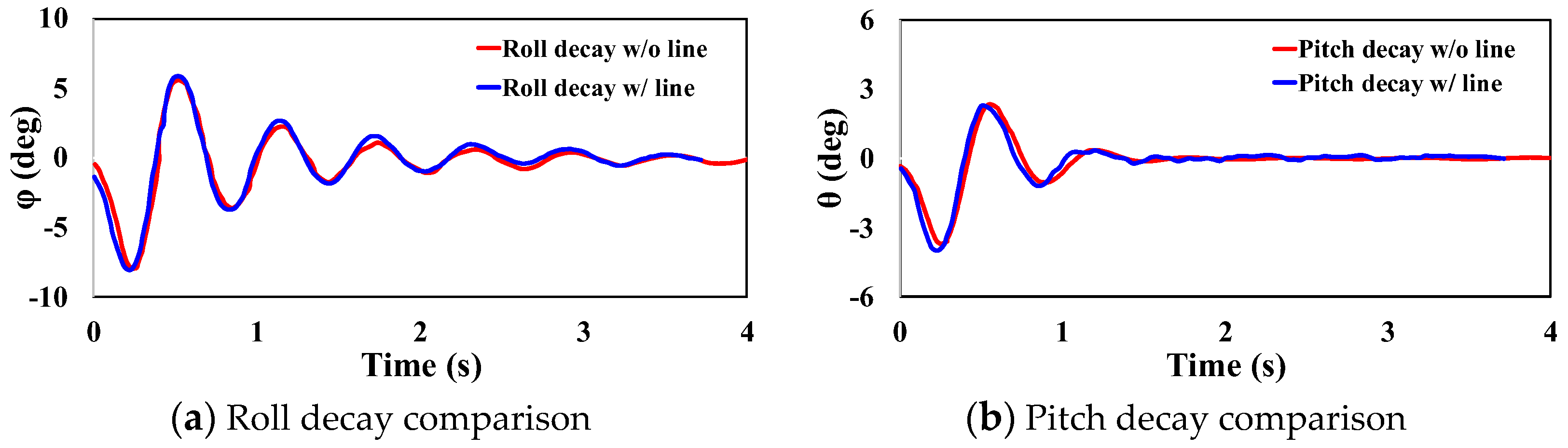
2.4. Experiment for Validation

The experiment was performed to verify the RAO predicted through CMP. The experiment was conducted in a physical wave tank with a length of 20 m, a width of 14 m, and a water depth of 19.5 m, consistent with Nam et al. [14]. The wave absorber was installed on the opposite side of the wave maker to prevent the reflection of incoming waves from the boundary of the wave basin and to implement the assumption of interaction between floating bodies and waves within the infinite range of the fluid [34]. The model scale was 1/49. As shown in Figure 10, a free-floating model was installed, allowing for unrestricted 6-DOF motion through the use of a soft spring. Tension gauges were employed to measure the wave forces acting on the ship model. These gauges were connected to the ship at four angle positions of the support frame to ensure balance. Once the tension gauges were installed, soft springs and lines were connected to the model ship. According to the International Towing Tank Conference (ITTC) recommendation [35], the model ship can be restrained in surge or towed using a spring system. The spring stiffness should be selected to result in a resonance frequency at least twice as low as the lowest wave encounter frequency. In compliance with this recommendation, a spring stiffness of 9 N/m was chosen, which satisfied the surge and sway motion compared to the reference encounter frequency. The experimental setup, including the connection equipment, may introduce factors that are not accounted for in simulations, particularly when considering a free-floating body. Therefore, a roll and pitch decay test was performed to compare the motion with or without lines. The results of the decay test are indicated in Figure 11, confirming that the motions align well irrespective of the presence of lines. For the measurement of 6-DOF motion in this experiment, an optics-based system (V120:TRIO, OptiTrack, Corvallis, OR, USA) and inertial measurement unit (IMU) sensors were used.

To conduct the tests on the model scale in regular waves, the full-scale conditions needed to be scaled accordingly. Following the principles of Froude similarity represented by Equation (13), a ship design speed condition of 0.441 m·s⁻¹ was employed at the model scale. In Equation (13), $V$ and $L$ are the velocity and length of a barge, respectively. The subscript $s$ indicates the full scale, while $m$ means the model scale parameter.

$$F_n=\frac{V_s}{\sqrt{g_s{L}_s}}=\frac{V_m}{\sqrt{g_m{L}_m}}$$

(13)

Regular waves within a range of 4.55–12.60 rad·s⁻¹ were generated at the model scale for the motion test. The determination of wave height for each frequency followed the recommendation of the ITTC for seakeeping experiments [35]. In this recommendation, the wave height must be chosen such that the condition ‘wave height/wavelength < 1/50’ (small wave slope) is satisfied, ensuring results consistent with linear surface-wave theory. The model ship, which is symmetrical along the x-axis, underwent testing in a total of seven directions at 30° intervals, ranging from 180° (bow) to 0° (stern). The waves were generated in the same direction using the wave maker, while the towing carriage was moved simultaneously in the forward, backward, left, and right directions within the tank to simulate multi-directional regular waves for the ship.

Figure 10. Model installation for experiment.

Figure 10. Model installation for experiment.

Figure 11. Comparison of motion with and without lines.

Figure 11. Comparison of motion with and without lines.

3. Results and Discussion

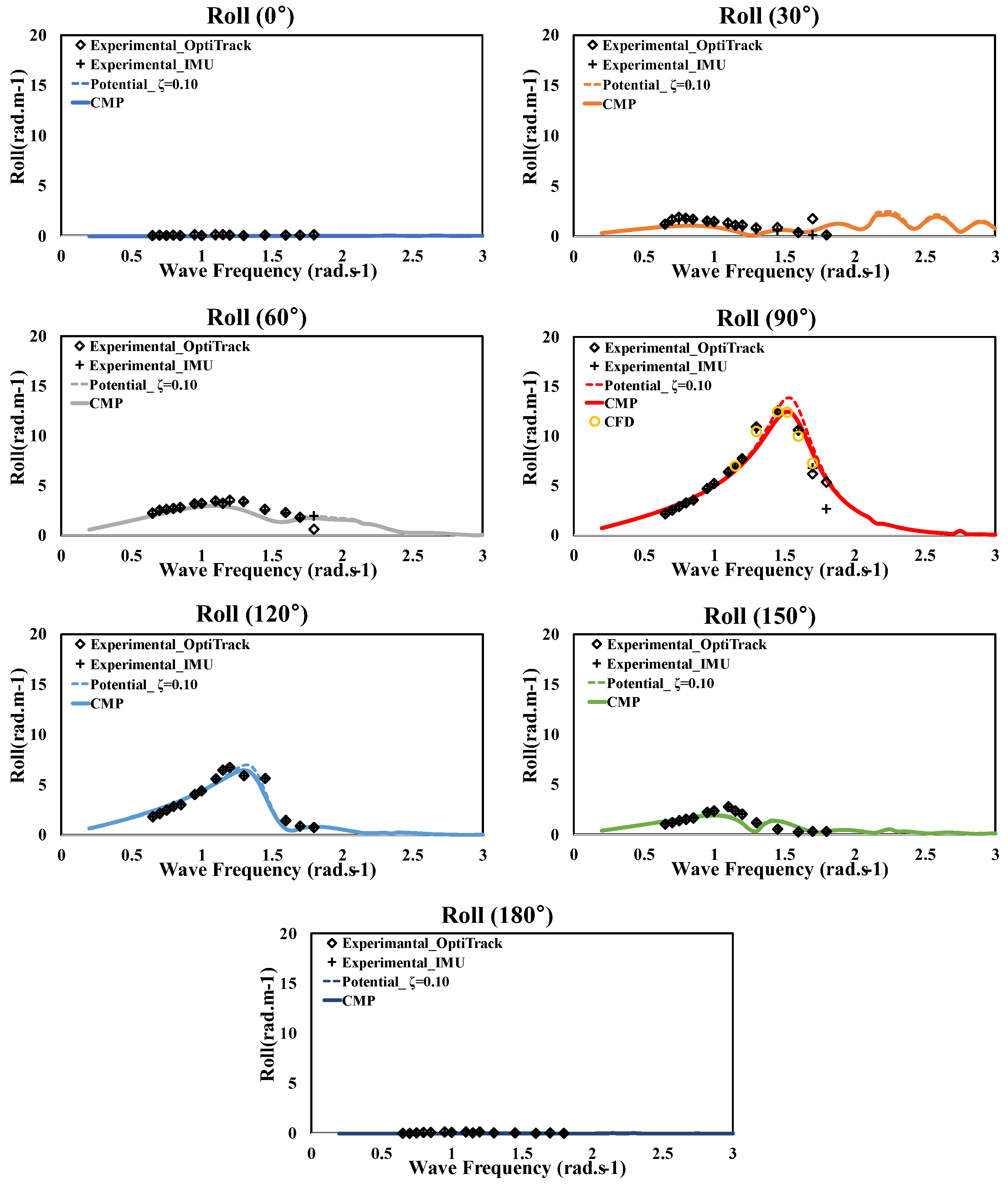
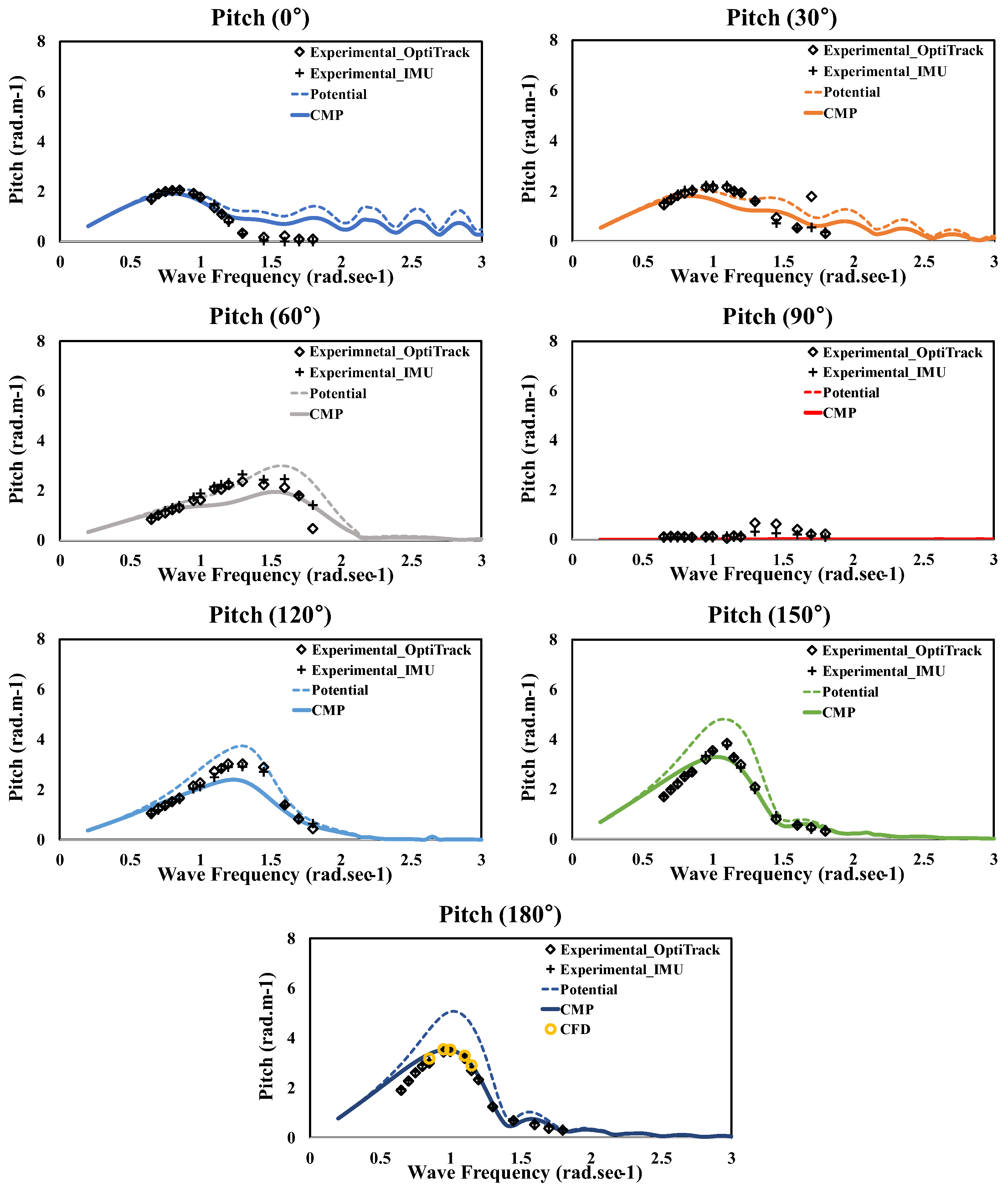
3.1. Results of RAOs

Figure 12 and Figure 13 illustrate the results of the RAOs of roll and pitch in each wave direction. In the experimental results, the circle represents the optics-based system, and the cross represents the motion test results for each frequency measured by the IMU sensor. Furthermore, a damping ratio of 0.1 for the potential flow program result is depicted by a dotted line, while the thickest solid line represents the analysis result using the CMP model. In the figures, “CFD”, indicated by yellow circles, refers to the results of full CFD simulations performed independently for roll and pitch at 90° and 180° wave directions, respectively. First, upon comparing the RAO results of the CMP model for 90° roll and 180° pitch with those from the potential flow program applying an initial damping coefficient of ζ = 0.10, it is observed that the CMP model more closely aligns with the experimental results. More specifically, the results of the CMP model show relative errors of approximately 3.5% in period and 1.2% in amplitude at the 90° roll peak (1.5 rad·s⁻¹), compared to the experimental data. At the pitch 180° peak (1.0 rad·s⁻¹), the period was exactly the same, and the amplitude showed a relative error of 5.2%. In other words, it can be confirmed that by using the CMP model, almost the same results as the experiment can be obtained even in situations where the damping ratio of the ship is unknown. For additional verification, the full CFD simulations were performed at four to five frequencies, including the peak frequencies for 90° roll and 180° pitch. These simulations confirmed that an error in the range of approximately 1 to 5% occurred. Through this, it was possible to cross-check that the results of motion analysis using CFD show relative reliability. However, as a full CFD simulation is time-intensive, the CMP model offers a faster and more reliable alternative when time constraints are present.

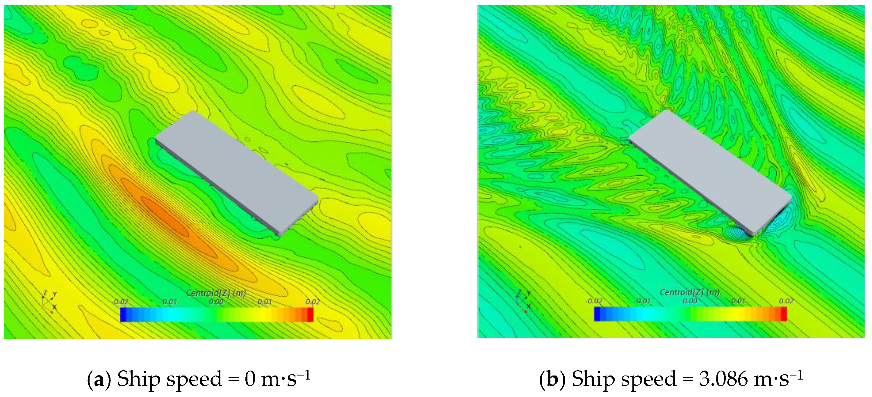
3.2. Results of Seakeeping Performance

Following the procedure outlined in the fourth stage of Section 2.3 above, seakeeping performance was evaluated in the target sea area. Figure 14 illustrates the seakeeping performance results for roll and pitch in various sea states. To validate the seakeeping performance using the CMP model, a comparison was made between these results and those obtained from a potential flow program incorporating an arbitrary damping ratio of 0.10, as well as the experimental model test results. The seakeeping performance achieved through the potential flow program is represented by the black dotted line, while the red line illustrates the intended result using the CMP model in this study. The green diamond symbols in each wave direction indicate the experimental results obtained from IMU. The analysis of seakeeping performance in this study was conducted from 0° to 180°. However, the wave directions from 180° to 360° are displayed symmetrically as the target barge is x-axis symmetric.

In the case of roll motion, it is seen clearly that the CMP results align more closely with the experimental results across all sea states, in contrast to the results yielded by the potential flow program. This implies that the CMP results can be deemed a more reliable model in comparison to prevalent potential flow programs that are currently employed in a plethora of seakeeping analyses. On the other hand, in the case of pitch, the CMP results show underestimated values in almost all wave directions compared to the experiments, and the results of the potential flow program are closer to the experimental results. In addition, for a wave direction of 90°, unlike the experiment, it can be confirmed that the values of both simulations are close to 0 across all sea states. Referring to Figure 15 for a wave direction of 90°, which reproduced by CFD the flow around the ship under the same conditions as the experiment, it can be observed that a difference in wave height generated at the bow and stern as the speed increases and the resulting pressure difference on the hull occur. In essence, it can be understood that when the ship is advanced and waves approach from a 90° direction, trimming occurs due to the disparity in hydrodynamic forces exerted on the stern and bow, consequently leading to an increase in pitch motion. Not adequately capturing these physical phenomena is recognized as a limitation of potential theory-based models, and it will require correction and supplementation in future research endeavors.

For a more comprehensive analysis of the results, the relative error was compared with the experimental results, particularly under conditions where the SSA was the most pronounced. It was confirmed that the wave direction of 90° for roll and 180° for pitch exhibited the highest SSA values based on the seakeeping performance analysis.

Table 6. Relative error of seakeeping performance result with experiment.

Evaluation Items (Wave Direction)	Analysis Method	Sea State 2 Relative Error (%)	Sea State 3 Relative Error (%)	Sea State 4 Relative Error (%)
Roll (90°)	Potential	80	59	68
	CMP	15	6	1
Pitch (180°)	Potential	27	22	37
	CMP	10	12	13

presents the relative error according to each sea state, compared to the corresponding wave direction conditions. In the case of a roll at 90°, the potential flow program results showed a substantial discrepancy ranging from 59% to 80% across all sea states. In contrast, CMP yielded an error of 1% to 15%, with a trend of decreasing errors as sea state increased. In pitch at 180°, the potential flow program results demonstrated a tendency to overpredict compared to the experiment, reflecting errors ranging from 22% to 37% across all sea states. Conversely, CMP showed smaller errors of 10% to 13% compared to the potential flow program, yet a tendency to underpredict was also observed.

4. Conclusions

In this study, the CMP method, a simulation procedure proposed by Nam et al. (2022) [14], was employed to predict the motion RAOs of a barge under a wide range of sea states, and then seakeeping performance was evaluated based on these motion results. The reliability of the motion analysis results obtained using CMP was verified by comparing them with the results from the experiments, potential flow program, and full CFD simulations. Specifically, at the peak where maximum motion occurs, the RAOs of the CMP model were compared with those of the potential flow program applying an initial damping coefficient determined empirically. As a result, in the case of roll, the potential flow program exhibited an error of 6.9% in period and 9.9% in amplitude, whereas the CMP model showed an error of 3.5% in period and 1.2% in amplitude. In the case of pitch, while all periods were consistently the same, the potential flow program demonstrated an error of 41.6% in amplitude, compared to 5.2% in amplitude for the CMP model. This suggests that more reliable results can be achieved through motion analysis of the barge using the CMP model, particularly when the initial damping ratio required for analysis using the potential flow program is not predetermined. Subsequently, seakeeping performance was analyzed based on SSA values. And the results were compared under specific wave direction conditions (90° for roll and 180° for pitch), where SSA was most prominent in each respective motion. For the 90° roll, the results from the potential flow program displayed significant discrepancies, with error margins reaching 59–80% across all sea states. Conversely, in the case of the CMP model, errors were more contained, ranging from approximately 1 to 15%. Notably, as the sea state intensified, the error margin demonstrated a tendency to decrease. For the 180° pitch, the potential flow program results tended to overpredict compared to the experiment, with errors ranging from 22% to 37% across all sea states. In contrast, the CMP model exhibited errors of 10–13% but showed a tendency to underpredict. Consequently, this demonstrates that applying the CMP model for analyzing seakeeping performance of barges under conditions where SSA is most prominent can yield more accurate results than those obtained from potential flow programs.

In this study, the CMP model was applied exclusively to a barge. However, future research could investigate its applicability to a broader spectrum of ship types and forms, offering a significant contribution to the field.

References

1. Chun, H.H.; Chun, S.H.; Kim, S.Y. Roll damping characteristics of a small fishing vessel with a central wing. Ocean. Eng. 2001, 28, 1601–1619. [Google Scholar] [CrossRef]
2. Prini, F.; Benson, S.; Birmingham, R.W.; Dow, R.S.; Phillips, H.J.; Sheppard, P.J.; Varas, J.M. Seakeeping analysis of a high-speed search and rescue craft by linear potential theory. In Proceedings of the International Conference on Lightweight Design of Marine Structures, Glasgow, UK, 9–11 November 2015; pp. 87–96. [Google Scholar]
3. Sclavounos, P.D.; Borgen, H. Seakeeping analysis of a high-speed monohull with a motion-control bow hydrofoil. J. Ship Res. 2004, 48, 77–117. [Google Scholar] [CrossRef]
4. Lewandowski, E.M. Multi-vessel seakeeping computations with linear potential theory. Ocean Eng. 2008, 35, 1121–1131. [Google Scholar] [CrossRef]
5. Zhang, X.; Bandyk, P.; Beck, R.F. Seakeeping computations using double-body basis flows. Appl. Ocean Res. 2010, 32, 471–482. [Google Scholar] [CrossRef]
6. Jung, K.H.; Chang, K.A.; Huang, E.T. Two-dimensional flow characteristics of wave interactions with a free-rolling rectangular structure. Ocean Eng. 2005, 32, 1–20. [Google Scholar] [CrossRef]
7. Toxopeus, S.; Sadat-Hosseini, H.; Visonneau, M.; Guilmineau, E.; Yen, T.G.; Lin, W.M.; Grigoropoulos, G.; Stern, F. CFD, potential flow and system-based simulations of fully appended free running 5415M in calm water and waves. Int. Shipbuild. Prog. 2018, 65, 227–256. [Google Scholar] [CrossRef]
8. Niklas, K.; Karczewski, A. Determination of seakeeping performance for a case study vessel by the strip theory method. Pol. Marit. Res. 2020, 27, 4–16. [Google Scholar] [CrossRef]
9. Simonsen, C.D.; Otzen, J.F.; Joncquez, S.; Stern, F. EFD and CFD for KCS heaving and pitching in regular head waves. J. Mar. Sci. Technol. 2013, 18, 435–459. [Google Scholar] [CrossRef]
10. Im, N.; Lee, S. Effects of Forward Speed and Wave Height on the Seakeeping Performance of a Small Fishing Vessel. J. Mar. Sci. Eng. 2022, 10, 1936. [Google Scholar] [CrossRef]
11. Ozturk, D.; Delen, C.; Mancini, S.; Serifoglu, M.O.; Hizarci, T. Full-scale CFD analysis of double-m craft seakeeping performance in regular head waves. J. Mar. Sci. Eng. 2021, 9, 504. [Google Scholar] [CrossRef]
12. Fitriadhy, A.; Dewa, S.; Mansor, N.A.; Adam, N.A.; Ng, C.Y.; Kang, H.S. CFD investigation into seakeeping performance of a training ship. CFD Lett. 2021, 13, 19–32. [Google Scholar] [CrossRef]
13. Kim, Y.; Park, J.B.; Park, J.C.; Park, S.K.; Lee, W.M. Development of an evaluation procedure for seakeeping performance of high-speed planing hull using hybrid method. J. Soc. Nav. Archit. Korea 2019, 56, 200–210. [Google Scholar] [CrossRef]
14. Nam, S.; Park, J.C.; Park, J.B.; Yoon, H.K. CFD-Modified Potential Simulation on Seakeeping Performance of a Barge. Water 2022, 14, 3271. [Google Scholar] [CrossRef]
15. Faltinsen, O.M. Sea Loads on Ships and Offshore Structures; Cambridge University Press: London, UK, 1990; p. 328. ISBN 0-521-45870-6. [Google Scholar]
16. Sariöz, K.; Narli, E. Effect of criteria on seakeeping performance assessment. Ocean Eng. 2005, 32, 1161–1173. [Google Scholar] [CrossRef]
17. Korea Maritime Safety Tribunal. Statistics of Marine Accident. 2020. Available online: https://www.kmst.go.kr/eng/com/selectHtmlPage.do?htmlName=m4_vesseltype (accessed on 1 December 2021).
18. Suh, K.D.; Kwon, H.D.; Lee, D.Y. Statistical characteristics of deepwater waves along the Korean Coast. J. Korean Soc. Coast. Ocean Eng. 2008, 20, 342–354. [Google Scholar]
19. Bouws, E.; Günther, H.; Rosenthal, W.; Vincent, C.L. Similarity of the wind wave spectrum in finite depth water: 1. Spectral form. J. Geophys. Res. Ocean. 1985, 90, 975–986. [Google Scholar] [CrossRef]
20. Kitaigordskii, S.A.; Krasitskii, V.P.; Zaslavskii, M.M. On Phillips’ theory of equilibrium range in the spectra of wind-generated gravity waves. J. Phys. Oceanogr. 1975, 5, 410–420. [Google Scholar] [CrossRef]
21. Goda, Y. Random seas and design of maritime structures. Adv. Ser. Ocean Eng. 2000, 15, 25–30. [Google Scholar]
22. Thompson, E.F.; Vincent, C.L. Prediction of Wave Height in Shallow Water. In Proceedings of the Specialty Conference on the Design, Construction, Maintenance, and Performance of Coastal Structures—Coastal Structures ’83, Arlington, TX, USA, 9–11 March 1983; pp. 1000–1008. [Google Scholar]
23. Det Norske Veritas. Offshore Standard DNV-OS-E301 Position Mooring; Det Norske Veritas: Bærum, Norway, 2010. [Google Scholar]
24. Lloyd’s Register. WAVELOAD-FD User Manual, Version 1.1 for User of ShipRight and ShipRight-FOI; Lloyd’s Register: Southampton, UK, 2015. [Google Scholar]
25. ABS (American Bureau of Shipping). Guidance Notes on ‘Dynamic Load Approach’ and Direct Analysis for High Speed Craft; ABS (American Bureau of Shipping): Houston, TX, USA, 2003. [Google Scholar]
26. Zaidi, H.; Fohanno, S.; Taiar, R.; Polidori, G. Turbulence model choice for the calculation of drag forces when using the CFD method. J. Biomech. 2010, 43, 405–411. [Google Scholar] [CrossRef] [PubMed]
27. Kim, J.I.; Park, I.R.; Suh, S.B.; Kang, Y.D.; Hong, S.Y.; Nam, B.W. Motion Simulation of FPSO in Waves through Numerical Sensitivity Analysis. J. Ocean Eng. Technol. 2018, 32, 166–176. [Google Scholar] [CrossRef]
28. Jiao, J.; Huang, S. CFD simulation of ship seakeeping performance and slamming loads in bidirectional cross wave. J. Mar. Sci. Eng. 2020, 8, 312. [Google Scholar] [CrossRef]
29. Jung, D.; Kim, S. Computational Investigation of Seakeeping Performance of a Surfaced Submarine in Regular Waves. J. Ocean. Eng. Technol. 2022, 36, 303–312. [Google Scholar] [CrossRef]
30. Roache, P.J. Perspective: A method for uniform reporting of grid refinement studies. J. Fluids Eng. 1994, 116, 405–413. [Google Scholar] [CrossRef]
31. Roache, P.J. Quantification of uncertainty in computational fluid dynamics. Annu. Rev. Fluid Mech. 1997, 29, 123–160. [Google Scholar] [CrossRef]
32. NORDFORSK. Assessment of Ship Performance in a Seaway, Nordic Cooperative Project: Seakeeping Performance of Ships; NORDFORSK: Copenhagen, Denmark, 1987; p. 32. [Google Scholar]
33. NATO (North Atlantic Treaty Organization). Common Procedures for Seakeeping in the Ship Design Process, 3rd ed.; STANAG 4154; NATO (North Atlantic Treaty Organization): Washington, DC, USA, 2000. [Google Scholar]
34. Youn, D.; Choi, L.; Kim, J. Motion Response Characteristics of Small Fishing Vessels of Different Sizes among Regular Waves. J. Ocean Eng. Technol. 2023, 37, 1–7. [Google Scholar] [CrossRef]
35. ITTC. Recommended Procedures and Guidelines. Seakeeping Experiments. In Proceedings of the 27th ITTC Seakeeping Committee, Copenhagen, Denmark, 1–5 September 2014; pp. 1–22. [Google Scholar]
Figure 1. Target barge.
Jmse 12 00369 g001
Figure 2. TMA spectrum.
Jmse 12 00369 g002
Figure 3. Computational procedure of CMP model by Nam et al. (2022) [14].
Jmse 12 00369 g003
Figure 4. Potential flow program mesh configuration.
Jmse 12 00369 g004
Figure 5. Numerical tank size CFD simulation.
Jmse 12 00369 g005
Figure 6. Detailed mesh scene of near the hull and free surfaces.
Jmse 12 00369 g006
Figure 7. Mesh configuration and boundary.
Jmse 12 00369 g007
Figure 8. Results of grid convergence test and calculated GCI.
Jmse 12 00369 g008
Figure 9. Procedure of finding final damping ratio.
Jmse 12 00369 g009
Figure 12. Comparison of roll RAO.
Jmse 12 00369 g012
Figure 13. Comparison of pitch RAO.
Jmse 12 00369 g013
Figure 14. Azimuth diagram of seakeeping performance.
Jmse 12 00369 g014
Figure 15. Wave contour in wave direction of 90°.
Jmse 12 00369 g015