Abstract
The digitization of catch information for the promotion of sustainable fisheries is gaining momentum globally. However, the manual measurement of fundamental catch information, such as species identification, length measurement, and fish count, is highly inconvenient, thus intensifying the call for its automation. Recently, image recognition systems based on convolutional neural networks (CNNs) have been extensively studied across diverse fields. Nevertheless, the deployment of CNNs for identifying fish species is difficult owing to the intricate nature of managing a plethora of fish species, which fluctuate based on season and locale, in addition to the scarcity of public datasets encompassing large catches. To overcome this issue, we designed a transferable pre-trained CNN model specifically for identifying fish species, which can be easily reused in various fishing grounds. Utilizing an extensive fish species photographic database from a Japanese museum, we developed a transferable fish identification (TFI) model employing strategies such as multiple pre-training, learning rate scheduling, multi-task learning, and metric learning. We further introduced two application methods, namely transfer learning and output layer masking, for the TFI model, validating its efficacy through rigorous experiments.
1. Introduction
With the dwindling of marine resources owing to overfishing, the fisheries industry is striving to conserve and rejuvenate these resources through resource management, ensuring that fishing activities do not exceed the limits of natural reproduction. In 2018, the Japanese Fishery Act was modified after 70 years, with the objective of fostering sustainable fisheries. The most notable feature of this modification was its commitment to preserving and restoring resources through scientifically backed resource management, which necessitates the establishment of objectives rooted in empirical evidence. As depicted in Figure 1, effective resource management comprises four critical components:
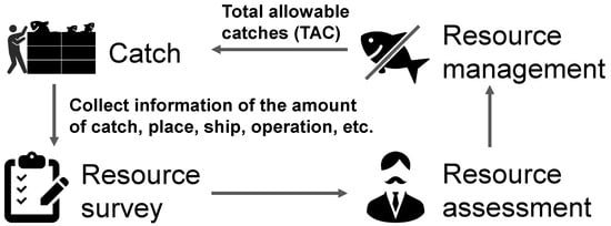
Figure 1.
Cycle of fish resource management.
- Resource survey:
- Collection of detailed catch information, including the quantity of fish, species, length, location, and fishing operations.
- Resource assessment:
- Estimating the condition of a fishery resource to determine its sustainability.
- Resource management:
- Coordinating with stakeholders and establishing control thresholds such as total allowable catch (TAC) based on various indicators.
- Catch:
- Fishing the following year in accordance with the resource management thresholds set.
The initial entry point into resource management, i.e., the collection of detailed catch information, is currently conducted manually by staff at each Prefectural Fisheries Experimental Station. To avoid obstructing the fisherman’s daily operations, the species type and length must be recorded in less than an hour from the time of landing to the auction. This small timeframe limits the number of samples that can be measured, considerably burdening the personnel. Moreover, under the revised Japanese resource management rule, the target species count has been expanded to 192. Manual data collection presents challenges in terms of both timeliness and accuracy in resource surveys.
The primary objective is to automate the task of recording the species and length of catches in resource surveys using image recognition. The proposed system aims to identify both species and length by capturing overhead imagery of each fish, as exemplified in Figure 2. Garcia et al. [1] employed Mask R-CNN for such measurements, albeit it necessitated extensive annotations (mask and species labels.) Alternatively, we [2] developed a system to automatically measure the number and length of fish through an instance segmentation technique using images of fish on a conveyor belt. Through copy–paste augmentation, the system can easily be specialized to various fishing grounds by preparing background images and a few annotated fish images, as shown in the lower left-hand corner of Figure 2. Our previous study [2] concentrated solely on detecting fish regions, thereby not incorporating the functionality to automatically identify fish species—critical for resource surveys. Additionally, identifying fish species, a task that involves distinguishing between species with highly similar appearances like Scomber japonicus Houttuyn and Scomber australasicus Cuvier, is classified as a fine-grained image recognition task—among the more challenging aspects of image recognition. Consequently, this study aims to develop a highly accurate model for identifying fish species from images, where fish regions have already been extracted by earlier studies, including [2]. By integrating a depth camera, the length of the fish can be estimated from the information on the fish region. While related studies, like those involving Mask R-CNN, employ a single model to estimate both fish species and regions [3], this study distinguishes itself by developing an independent model specifically designed for fish species identification. An advantage of this study is its requirement of only fish species labels, in contrast to related studies that necessitate preparing a large number of both fish species and region labels. Furthermore, another advantage is the superior detection performance of a model specialized in fish species identification, like the one developed in this study, compared to an all-in-one model like Mask R-CNN. On the downside, the model’s larger size and slightly increased inference time are drawbacks; however, these issues are not significant when considering the model’s application in resource surveys.
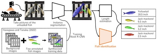
Figure 2.
Process flow of the system we are aiming to develop. This study focuses on only fish identification. Mask R-CNN is trained by the method we proposed previously [2].
In fishery resource surveys, the construction of individual datasets for various fishing grounds is impractical given that the fish types that can be caught fluctuate based on a multitude of factors, including season, location, and fishing method. As of 2023, more than 36,000 species of fish have been identified globally, with new species still being discovered. Over 4700 species of fish have been estimated to inhabit the waters around Japan. Even if the survey is narrowed to resource survey targets, staff must identify up to 192 species. Therefore, there is a demand for a model that covers a vast array of fish species or a base model that can easily be specialized to each fishing ground with minimal additional data training.
Fish species recognition can be conceptualized as an image classification challenge and can be addressed through the use of deep learning models typically applied to general image classification. As demonstrated in Table 1, image datasets of catches are gradually becoming more available. Preparing such image datasets has led to the development of many fish species identification models, as shown in Table 2. For instance, fish species identification models using original feature extraction or Convolutional Neural Networks (CNNs) have been developed [4,5,6]. Identification models by transfer learning using a pre-trained model of ImageNet [7] have also been developed [8,9,10,11,12,13]. These studies were conducted assuming that the training data, as shown in the column “target task”, are provided in each fishing ground; therefore, users need to prepare a new dataset and additionally train the model at the new fishing ground when they want to apply the model to a new place. Their research investigates unique techniques combined with CNNs; however, as far as we know, a transferable fish species identification model is yet to be developed using these datasets, partly because a large image dataset for landed fish has not yet been developed. In other words, most studies have assembled datasets specific to particular fishing grounds and trained models accordingly. In this study, we define a method that involves constructing a large dataset and training a specialized model for each fishing ground as a “specialized model”. In contrast, a method that either does not require additional training for each fishing ground or can be easily adapted by incorporating a small dataset is defined as a “transferable model”.
Moreover, biological image datasets frequently exhibit class imbalances, with varying numbers of data points per class. To address this issue, Alba et al. introduced a novel loss function for the single-shot multibox detector (SSD) powered by MobileNetV3, aimed at mitigating the class imbalance problem, and their evaluation confirmed its efficacy [14]. Additionally, Khan et al. developed FishNet, a comprehensive and varied aquatic species dataset designed to facilitate the creation of an automated monitoring system for aquatic species [15]. FishNet encompasses not only bio-class information but also supplementary data like bounding box (bbox) annotations as accurate labels. They also assessed the performance of CNN architectures such as ConvNeXt across various loss functions—cross-entropy loss (CE Loss), focal loss, and class balanced loss—specifically designed to address class imbalances.

Table 1.
Detailed information of public fish datasets.
Table 1.
Detailed information of public fish datasets.
| Citation | Dataset | # of Species | # of Images | Labels | Location |
|---|---|---|---|---|---|
| [16] | fish4Knowledge | 23 | 27,142 | S | Underwater |
| [17] | LifeCLEF 2015 Fish | 15 | >20,000 | S, B | Underwater |
| [18] | WildFish | 1000 | 54,459 | S | Underwater |
| [19] | WildFish++ | 2348 | 103,034 | S, D | Underwater |
| [20] | Fish-Pak | 6 | 915 | S | Landed |
| [21] | LargeFish | 9 | 430 | S, I | Landed |
| [22] | URPC | 4 | 3701 | S | Underwater |
| [23] | DeepFish | 59 | 1291 | S, I | Landed |
| [24] | SEAMAPD21 | 130 | 28,328 | S, B | Underwater |
| [15] | FishNet | 17,357 | 94,778 | S, B | Underwater, Landed |
S: species; B: bounding box; D: descriptions; I: instance mask.
Table 2.
Examples of fish species identification model development.
Table 2.
Examples of fish species identification model development.
| Citation | Target Task | Model | Pre-Train |
|---|---|---|---|
| [4] | Original | NN | None |
| [5] | Fish4Knowledge | CNN (2 layers) | None |
| [8] | Original | Inception v3 | ImageNet |
| [6] | Fish-Pak | CNN (32 layers) | None |
| [9] | Fish4Knowledge | ResNet50 | ImageNet |
| [10] | Fish4Knowledge | Inception v3 | ImageNet |
| [11] | LifeCLEF 2015 Fish | ResNet50 | ImageNet |
| [12] | LifeCLEF 2015 Fish & URPC | ResNet50 | ImageNet |
| [25] | Original | VGG16 | Unknown |
| [13] | Large Fish | MobileNetV2 | ImageNet |
| [14] | SEAMAPD21 | MobileNetV3 | Unknown |
| [15] | FishNet | ConvNeXt | ImageNet |
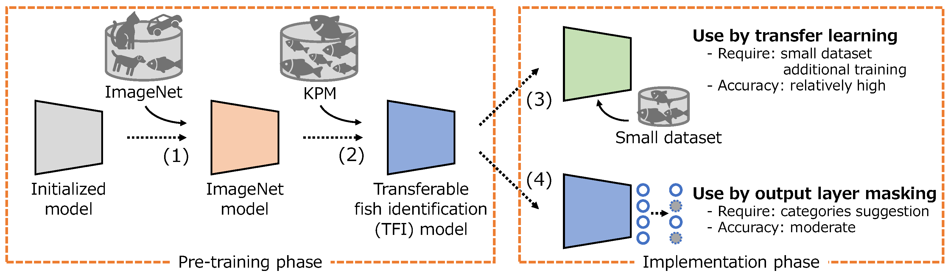
Based on the above, we develop a new transferable fish identification (TFI) model that can be easily applied to various fishing grounds as shown in Figure 3. The proposed method consists of two phases: pre-training and implementation. In the implementation phase, after training the deep learning model using the general object recognition dataset ImageNet1k ([7]), the TFI model is developed by additionally training on a large dataset of fish identification. The TFI model can be adapted for various fishing grounds using transfer learning. This necessitates further training with a modest dataset to achieve a relatively high accuracy. Alternatively, output layer masking can be used, in which case a fish species identification model can be developed without additional training, just using category suggestion of the target species. The detailed procedures are described in Section 2.2.1 and Section 2.2.2. In conventional research cases, fish identification models are developed using models pre-trained using ImageNet and conducting additional training at each fishing ground. However, as ImageNet only has a few fish classes, it is difficult to use a model pre-trained on ImageNet as a fish species classifier without additional training. Therefore, in the pre-training phase, we attempted to acquire feature representations specific to fish species identification using a large-scale dataset provided by the Kanagawa Prefectural Museum of Natural History (hereinafter, we call this dataset KPM), which contains approximately 200,000 images of 2826 fish species.
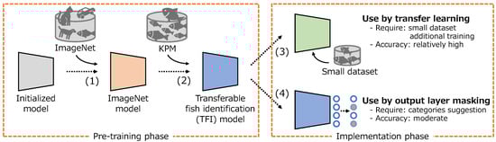
Figure 3.
Process flow to develop the transferable fish identification model and to apply to the various fishing grounds.
Extensive research has been conducted using multi-stage pre-training methods, especially in the medical field. Suzuki et al. [26] proposed a method to retrain models that have been pre-trained on ImageNet by using a textured image dataset, CUReT [27]. Transfer learning was then performed using a medical image classification dataset of CT. Zhang et al. [28] also proposed a multi-stage pre-training method to realize an image recognition model to support tongue examination, a traditional Chinese medical treatment. The concept of the aforementioned studies is based on two backgrounds. First, the cost of constructing a medical image dataset is extremely high. In addition, ImageNet is a general object recognition dataset, whereas medical image classification is a significantly different domain, and thus negative transfer is possible. Negative transfer [29] occurs when there exists a large divergence between the source and target domains, and, in this phenomenon, transfer learning inversely deteriorates the final accuracy of the target task. In contrast, our two-stage pre-training (ImageNet1k and KPM) could function similarly to curriculum learning [30], which is a kind of training strategy for deep learning models in which better feature representations are eventually obtained by sequentially training from easier tasks instead of randomly training a dataset.
The three main contributions of this study are as follows.
- We constructed a large fish identification dataset from images and labels provided by the Kanagawa Prefectural Museum of Natural History (KPM) and Zukan.com, Inc. KPM comprises approximately 200,000 images, each labeled with a type of fish species (Japanese name). Using this dataset with some training strategies, we developed a TFI model for various deep learning architectures.
- For the fish species identification task, the experimental results, using publicly available datasets, demonstrated that the developed model has better transfer performance than common pre-trained models using ImageNet.
- Experiments conducted on a subset of fish species of the Japanese resource survey revealed 129 fish species, with the proposed model achieving 72.9% accuracy without additional training.
2. Materials and Methods
2.1. Dataset Description
Before describing the proposed method, we describe the five datasets shown in Table 3 for model training and evaluation used in this study. These datasets were prepared by third parties and provided with permission; data availability is described at the end of this manuscript. We describe detailed collection methods in the following subsections.
Table 3.
Datasets we used in this study.
2.1.1. KPM
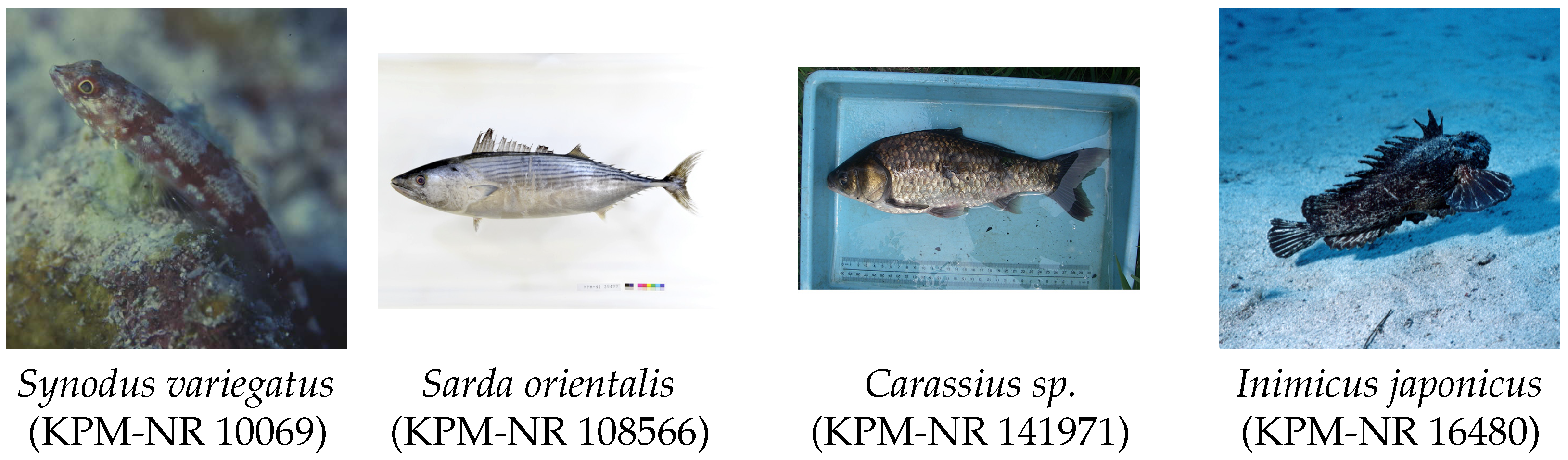
The KPM dataset was created from data registered in the fish photographic database1, which is managed and operated by KPM. We organized the registered fish photos and their metalabels to construct the dataset. By cooperating with the museum, we received all images and metalabels registered as of 25 August 2022. The resolution of all images is [px], and the dataset includes a wide range of images from specimens to underwater fishes. Essentially, while the images are primarily captured digitally, some data are converted from analog photographs. As depicted in Figure 4, the photographic environment, encompassing background and lighting, varies; hence, the images were captured under diverse conditions.
Figure 4.
Sample images of KPM dataset.
The total number of images are 287,587 images of 6708 species, including unidentified species; however, 196,293 images (2826 species) with at least 10 images of each species were selected for use. We resized all the images to [px]. The Japanese name of the species registered in the metalabels was used as the correct label. The fish species were manually identified by an ichthyologist; therefore, accuracy is guaranteed. In this study, the dataset was split into training and test sets using the hold-out method, with approximately 10% of the images from each species randomly selected for testing. This process yielded 176,819 images for training and 19,474 images for testing.
Biological classifications include class, order, family, genus, and species. Based on the Japanese names of the species, we manually labeled class, order, family, and genus of all 2826 target fish species using information from the Webfish dataset (described below) and manual references to databases outside Japan. The definitions of these classes may change from time to time, depending on ichthyological studies; however, we defined the labels based on the information available as of 2023.
2.1.2. Webfish
The Webfish dataset was created from data registered in the “Web Sakana Zukan” (visual dictionary of fish on Web)2, which is managed and operated by Zukan.com, Inc. With permission from the management company, images and information about the fish species were collected through scraping, around February 2023, and converted into a dataset. The images are not uniform in resolution and contain different backgrounds. Several images are of fish caught by anglers, and many were taken individually on the ground. However, some images show only a portion of the fish’s body, while others show multiple fish simultaneously.
As with KPM, we resized all images to [px]. Additionally, we used the Japanese names of the class, order, family, genus, and species provided in the service as the correct labels. In general, ichthyological experts evaluated the species identification to be accurate. Similarly to the KPM dataset, the Webfish dataset underwent a random division into training and test sets via the hold-out method, with about 25% of the images from each species selected randomly for testing. This division resulted in 29,134 images allocated for training and 10,335 images for testing.
Furthermore, we constructed a Webfish-small dataset by selecting fish species from the 192 included in Webfish and KPM, targeted for resource management in Japan. The Webfish-small dataset was used for the validation of the output layer masking and comprises 1171 images with 129 fish species (60 families and 106 genera).
2.1.3. Fish-Pak
The Fish-Pak dataset is a public dataset provided by Shah et al. [20]. It comprises 915 images of 6 fish species found in the waters of Pakistan. The dataset includes images of the entire body (body), face only (head), and scales only (scales). In the current study, we used only 271 images of the body. From this dataset, we randomly selected five images per class for testing, a total of 30 images. In addition, from the remaining images, we randomly selected k images from each class for training. The image resolution was 5184 × 3456 [px], and most of the images were taken in a monochromatic background environment. The name of the fish species (English name) was used for labeling, and all the images were resized to [px].
2.1.4. LargeFish
The LargeFish dataset is a public dataset provided by Ulucan et al. [21]. Here, 410 images of 9 fish species were gathered in a project at the Izmir University of Economics. We randomly selected 10 images per class for testing, 90 images in total, and then randomly selected k images from each class from the remaining images for training. The image resolution was set at 5184 × 3456 [px], and most were taken in a monochromatic background environment. Although segmentation labels were originally assigned, we used the name of the fish species (English name) as the correct label. All the images were then resized to [px].
2.2. Proposed Method
In this study, as described in the Introduction, the TFI model is developed using the pre-training phase (Figure 2). In addition, we propose a method to introduce the TFI model to various fishing grounds using a method such as the implementation phase (Figure 2). By conducting the pre-training phase on a high-performance server in advance, the TFI model can be applied to various fishing grounds for low-cost model adaptation by transfer learning and output layer masking, which can be used in different ways depending on specific circumstances of the fishing grounds. It should be noted that the purpose of this study is not to introduce a novel deep learning model architecture. Consequently, the accuracy might be enhanced further by employing techniques like DeepMAD [31] and BASIC-L [32], which have been posited as state-of-the-art for image recognition. Foundation models, such as CLIP [33], have been proposed recent year. However, fish identification model is difficult to adopt a foundation model because they are specialized to the general object classification task. We discuss about this in the Appendix A.
2.2.1. Pre-Training Phase
In the pre-training phase, we train a deep learning model two times as shown in Figure 2. Since we propose a training procedure, any deep learning model can be adopted, such as ResNet [34] and Swin Transformer [35]. The first pre-training of the 2-stage PT uses ImageNet, and the pre-trained weights have already been published in various deep learning libraries3. During the pre-training using ImageNet, various strategies have been employed, including RandAugment [36], cosine annealing warm restarts (CAWR, [37]), and label smoothing [38]. The training strategy and detailed hyperparameters for pre-training with ImageNet depend on the model provided by Pytorch and can be found in the official reference4. The second pre-training uses KPM dataset, and we employed training strategies such as RandAugment, CAWR, multi-task learning (MLT, [39]), and ArcFace Loss (AF Loss, [40]).
RandAugment [36] is a method of randomly applying various data augmentations with two hyperparameters: the number of applications, n, and their magnitude, m. This enab;es more efficient data augmentation than constant data augmentation.
CAWR [37] is a type of learning rate scheduler that decays the learning rate during learning according to a cosine curve, returns the learning rate to its original value after a certain period, and decays it again; this process is repeated. The method is expected to achieve the optimal solution to rapidly determine the local optimum solution and then exit it by returning the learning rate to reconduct the search.
MTL [39] is used to obtain better feature representation by using multiple outputs and multiple types of label information. In particular, the estimation accuracy may be improved using MTL for the biological classification of organisms, as proposed by Dhall et al. [41]. In addition, they compared a multi-output model with simultaneous class labels (called hierarchy-agnostic baseline classifier; HAB), an MTL method in which each class is trained in separate fully connected layers (called per-level classifier; PLC), and a method to compute the loss in the upper hierarchy by combining output values based on the hierarchical structure (called marginalization classifier; MC), with MC showing superior results. In contrast, our preliminary experiments using the fish dataset showed optimal results by using PLC. Therefore, MTL was adopted in this study with the hierarchical structure based on PLC.
AF Loss [40] is an angle-based metric learning method that can be implemented by adding a fully connected layer and using an improved softmax function. Based on angle between the feature map and weights of the fully connected layer, the loss function is such that the intraclass and interclass variances are small and large, respectively. In this study, we employed the AF Loss with 1024 dimensional embeddings, scale = 30 and margin = 0.5, for the mapping destination transformed in the fully connected layer. Although examples of metric learning applied to appearance-based fish species identification have not been found, Chen et al. [42] employed triplet loss, which is a type of metric learning method, for identifying fish species based on otoliths of fish. Yang et al. [43] adopted a supervised contrastive loss for plankton identification. Metric learning methods, such as ArcFace, were developed for detailed image classification tasks, such as human face recognition, and are expected to effectively identify fish species with similar appearances.
2.2.2. Implementation Phase
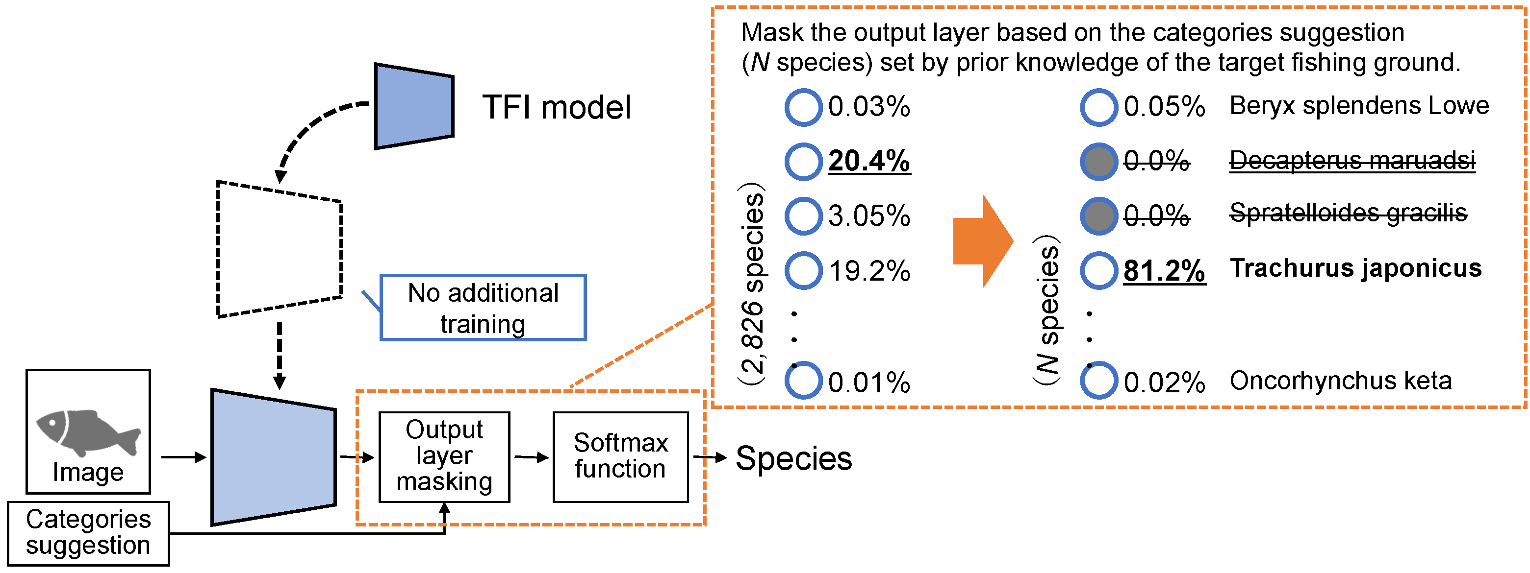
In the implementation phase, we adapted the TFI model for use across various fishing grounds. As depicted in Figure 2, this study proposes two strategies for adjusting the TFI model. One is fine-tuning, a type of transfer learning, while the other is output layer masking based on category suggestion.
In transfer learning, the TFI model is trained by fine-tuning using an additional dataset. Fine-tuning is a method for adjusting the pre-trained model to enhance its performance for a specific task. In this case, the specific task means the fish identification specified in the target fishing ground; therefore, we suppose that some images and correct labels in the target fishing ground are required as the additional dataset. This method can be used when users want to identify species other than the 2826 species that the TFI model can identify, or when users want to achieve a more accurate identification model for a few specific fish species. This method is inspired by Suzuki’s two-stage transfer learning [26]. In this study, we used CE loss, RandAugment, and CAWR in transfer learning.
In output layer masking, the TFI model is used without additional training. As shown in Figure 5, TFI model is used to identify species by masking the output layer to narrow down the output categories based on the category suggestion. Category suggestion is defined based on the expert’s knowledge for each fishing ground. For example, as Decapterus maruadsi and Trachurus japonicus are similar in appearance, the identification model could misclassify. However, based on a priori knowledge of the fishing ground, if Decapterus maruadsi cannot likely be caught, then a unit for this species is essentially not required in the output layer. Therefore, the output layer masking is a method in which only the category suggestion set based on prior knowledge is used as the output layer.
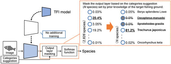
Figure 5.
Process outline of the output layer masking based on the category suggestion.
Output layer masking can be implemented with a simple process. First, a mask vector is created in advance based on category suggestion, with 1 for fish species that can be caught in the target fishing grounds and 0 for those that cannot be caught. The Adamar product of the mask vector and the scores of the 2826 fish species output by the TFI model are computed just before the softmax function is passed. The probability can be calculated appropriately by performing the masking just before the softmax function.
2.3. Experimental Settings
We outline the experimental setup used to assess the proposed method’s effectiveness. The experiments were conducted on a HPCDIY-ERMGPU8R4S workstation (HPC SYSTEMS Inc., Tokyo, Japan) equipped with dual AMD EPYC 7302 CPUs (Advanced Micro Devices, Inc., Santa Clara, CA, USA), 2TB of RAM, and six NVIDIA RTX A6000 GPUs (NVIDIA Corporation, Santa Clara, CA, USA). Our experiments utilized a conda Python (3.9.7) environment with the PyTorch (1.13.1) library for implementation. The model’s architecture and pre-trained weights were sourced from the standard torchvision library (0.14.1) offerings5. Pre-training on the KPM dataset, within this setup, varied from four to six hours per session, contingent on the chosen model architecture.
3. Results
We assessed the proposed method’s efficacy across multiple datasets from three distinct angles:
- Potential performance evaluation:
- We gauge the proposed model’s potential by examining its estimation accuracy on the KPM test set during pre-training with the KPM dataset (Section 3.1).
- Impact of pre-training:
- The effect of pre-training methods on transfer performance is evaluated. The robustness of our approach is showcased through the transfer performance analysis, comparing scenarios with large (Webfish dataset) versus small (Fish-pak and LargeFish datasets) additional training data, reflecting a “few-shot learning” context (Section 3.2).
- Performance without additional training:
- Our method’s performance is analyzed without additional training. This includes comparing direct inference using the TFI model to inference with output layer masking, incorporating prior knowledge (Section 3.3).
We first describe the common experimental setup used in the experiments to evaluate the effectiveness of each method. In the following experiments, unless otherwise noted, Adam was used as the optimizer with the learning rate of 5 × . The training was conducted for 100 epochs, and the results were evaluated using the micro F1-score6 on the test data after the last epoch of training. These experimental settings were established following basic hyperparameter tuning conducted during preliminary experiments. In this experiment, we used six model architectures: ResNet [34], EfficientNet [44], EfficientNet V2 [45], RegNet [46], Swin Transformer (Swin_T, [35]), and ConvNeXt [47]. Each model possesses different numbers of parameters; however, in this study, we used a model of a similar or smaller size compared to ResNet50. In each model, the encoder was used up to the output layer, and only the fully connected layer was replaced by a new single output layer.
3.1. Evaluation of Pre-Training Phase
We first evaluated the pre-training accuracy (2826 classifications) of the KPM dataset. Table 4 shows the results of training the KPM dataset under various conditions using ResNet50 (we used ResNet50’s weights of IMAGENET1K_V17) and CE Loss. The “KPM” and “WebFish” columns indicate the test scores in pre-training (KPM) and transfer learning (Webfish), respectively. We describe the results of transfer learning in the next section. Bold and underlined values indicate the best results for each condition. In terms of effectiveness, the following factors were compared: the presence or absence of ImageNet pre-training (Source), CAWR, and MTL. The results showed the practical effectiveness of ImageNet pre-training and CAWR, whereas the effect of the MTL was not significant. MTL can be used to simultaneously estimate the biological classifications and the species; therefore, it can be used to estimate the family and order, even when a detailed estimation of species is not necessary for operational purposes.
Table 4.
Performance comparison results for different pre-training strategies in pre-training (KPM) and transfer learning (Webfish) [%] (ResNet50 and CE Loss and lr = 5 × ).
Table 5 shows the results of evaluating the differences in model architecture and the number of parameters for each model provided by Pytorch. There are two types of ResNet50 in this table, meaning weights for which ResNet50 was trained with different training strategies (V1 and V28). Clearly, CAWR is still effective and Swin_T demonstrated the highest estimation accuracy for approximately the same model size.
Table 5.
Performance comparison results for different model architectures in pre-training (KPM) and transfer learning (Webfish) [%] (CE Loss and lr = 5 × ). The (8) KPM column means that each model is pre-trained under condition (8) in Table 4.
Furthermore, the results of validating AF Loss are shown in Table 6. Based on the results of prior validation, the learning rate was changed to 0.0001 when using both CE and AF Losses. When using AF Loss, the trend of CAWR and MTL contributing to improve the score remains consistent. Notably, the test score of KPM is marginally better with AF Loss than with CE Loss. On the other hand, in the context of ImageNet’s impact, pre-training with ImageNet significantly enhances performance when using CE Loss (Table 5). In contrast, with AF Loss, ImageNet pre-training appears to have little to no influence on performance improvement.
Table 6.
Performance comparison results for different loss functions in pre-training (KPM) and transfer learning (Webfish) [%] (Swin_T and lr = 1 × ).
3.2. Evaluation of Transfer Learning
3.2.1. Scenario When Relatively Large Dataset Is Available
We evaluated the effectiveness of the TFI model in transfer learning. First, we evaluated the transfer performance when a large number of data, such as 30,000 images of 1212 fish species, can be prepared in the target fishing ground, as in the case of the Webfish dataset. Table 4 shows the results with respect to the Webfish dataset. Fine-tuning was performed from the model corresponding to the “KPM-train strategy” columns. The table shows that a higher performance was achieved by fine-tuning the TFI model using ImageNet and KPM (5–8). The models with no pre-training (none) and fine-tuning from ImageNet achieved an accuracy of approximately 73%, whereas the model using only KPM without ImageNet in the pre-training resulted in lower estimation accuracy. Similarly, the comparison results of the impact of different model architectures are shown in Table 5. The estimation accuracy shown in Table 5 is almost of the same order as that of the pre-training, and the method using TFI model of Swin_T demonstrated the highest accuracy.
The “Webfish” column in Table 6 shows the comparative results of fine-tuning the Swin_T model with AF Loss. Interestingly, although AF Loss did not significantly affect pre-training, it contributed to an overall improvement in accuracy during fine-tuning, thus improving the accuracy by up to approximately 2% compared to the case of using the CE Loss. Highlighting the impact of pre-training, by adjusting the learning rate to 1 × , the un-pre-trained model faced challenges in effective learning, but incorporating ImageNet’s pre-training yielded an 81.8% accuracy. The TFI model, as shown, enhances the score by 2% with CE Loss and 4% with AF Loss. Remarkably, with AF Loss, a high score can be achieved without ImageNet’s pre-training weights, but a minor uptick of approximately 0.5% is observed when using ImageNet’s weights. Consistently, employing MTL and CAWR during pre-training improves transfer performance.
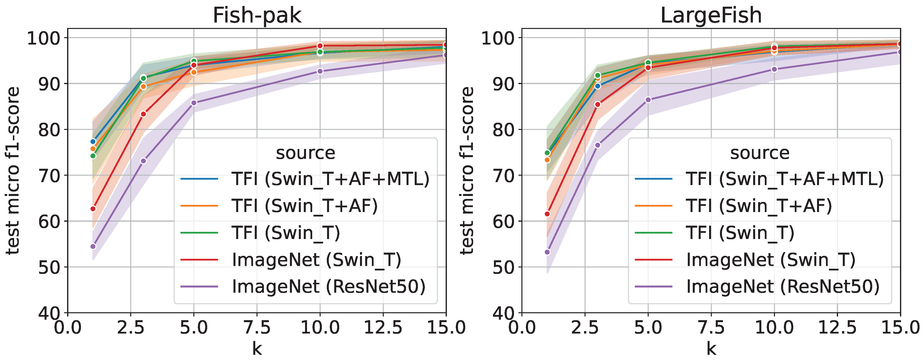
3.2.2. Scenario Involving Few-Shot Learning
To evaluate the performance of transfer learning by using the “few-shot” method, we evaluated the k-shot transfer performance using the Fish-Pak and LargeFish datasets, as shown in Figure 6. The term “few-shot” refers to the case where only a small amount of training data for each class are provided, and the parameter k denotes the number of images per class used for training. Originally, these two datasets did not have much training data; therefore, in this experiment, we conducted an evaluation experiment assuming a case in which only a small amount of training data can be prepared at the target fishing ground. The vertical axis of the figure is the micro F1-score [%] for the test data, and the horizontal axis is k for k-shot. Moreover, 10-trial means and 95% confidence intervals are shown because the results are sometimes unstable in the case of the “few-shot” dataset.
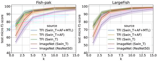
Figure 6.
Comparison results of k-shot fine-tuning using Fish-Pak and LargeFish datasets [%] (CAWR).
As shown in the figure, the TFI model is effective even in the case of few-shot learning. In this dataset, the overall estimation accuracy was higher for fine-tuning than for feature extraction; however, the trend remained the same. In both cases, the accuracy was improved by changing the encoder to Swin_T. In addition, the introduction of the TFI model, AF Loss, and MTL improved the estimation accuracy, especially when k was small.
3.3. Evaluation of Output Layer Masking
Table 7 shows the validation results, in which the TFI model was used in another fishing ground without additional training. In this experiment, we used the Webfish-small dataset as the test dataset, and Swin_T was trained using CAWR as the model. The center two columns show the test accuracy (micro F1-score) of identifying 2826 fish species by using the model as is. The right two columns show the accuracy (micro F1-score) of 129 fish species classified using the output layer masking.
Table 7.
Comparison results of output layer masking using the Webfish-small dataset (Swin_T, CAWR, Top N accuracy [%]).
The table shows that most of the 2826 fish identification models have an accuracy of approximately 50%, with the TFI model (AF+MTL) achieving the highest accuracy of 58.5%. The 2826 fish species include deep-sea fish and fish species not found around Japan, and the number of target fish species is extremely large to validate the result. Therefore, we believe that this result is reasonable. In contrast, the output layer masking, which simply masks the output layer, achieves an accuracy of 72.9 %. Furthermore, if the top five predictions are assumed to be acceptable, an accuracy of 90.2 % can be achieved. Although there is room for debate as to whether this accuracy is practical, the result is favorable for a model that can be used without additional training. The further discussion are described in Appendix B and Appendix C.
4. Conclusions
In this study, we developed a transferable fish species identification model that can easily be deployed in various fishing grounds through a TFI model trained by using our fish image dataset. In particular, we extensively validated the effectiveness of introducing CAWR, MTL, and AF Loss during pre-training. In contrast to the conventional method, which requires the preparation of additional training datasets for each fishing ground, the output layer masking can identify up to 2826 fish species by simply selecting the target species, without additional training. The transfer learning also demonstrates higher accuracy than the conventional approach. In particular, our TFI model based on Swin_T successfully improves the transfer performance by more than 10% in Webfish compared to ResNet50 pre-trained on ImageNet, which was commonly used in related studies. Therefore, improved accuracy can be expected when transferring in different fishing grounds compared to conventional methods. While some scenarios indicated that ImageNet pre-training was not pivotal in improving transfer performance, broadly, integrating all the proposed strategies consistently delivered superior results. Furthermore, the TFI model can be used simply by selecting the target species. Our experimental results indicate that, for the Webfish-small dataset, the TFI model achieved a micro f1-score of 72.9% in identifying 129 species. The methodology we proposed offers contributions beyond simply automating resource surveys; it also holds promise for marine biology research in several ways: (1) rapid species identification from collected samples and underwater footage; (2) real-time monitoring of ecosystems via periodic underwater camera surveillance analyzed; and (3) employing AI to accurately identify habitats of endangered species and detect instances of illegal fishing.
In addition, the evaluation dataset used in this study comprises data obtained on the ground in anticipation of its application to resource surveys; however, the accuracy of fish species identification must be validated under more severe conditions, such as images taken on board ships and in seine nets. Moreover, the optimum accuracy of a practical fish species identification method must be demonstrated from the viewpoint of the automation field of resource surveys and include a fail-safe operation method.
Author Contributions
Conceptualization, T.H.; Data curation, H.S.; Formal analysis, T.H.; Funding acquisition, T.H.; Investigation, T.H.; Methodology, T.H.; Project administration, T.H.; Resources, T.H.; Software, T.H. and K.K.; Supervision, T.H.; Validation, T.H. and K.K.; Visualization, T.H.; Writing—original draft, T.H.; Writing—review and editing, K.K. and H.S. All authors have read and agreed to the published version of the manuscript.
Funding
This work was supported in part by JST ACT-X grant number JPMJAX20AJ.
Institutional Review Board Statement
Not applicable.
Informed Consent Statement
Not applicable.
Data Availability Statement
The data underlying this article were provided by some organizations (KPM, Webfish, Fish-pak, and LargeFish datasets were provided by Kanagawa Prefectural Museum of Natural History, zukan.com, Inc., Shah et al. [20], and Ulucan et al. [21], respectively) via permission. Data will be shared directly from each organization by request to them.
Acknowledgments
The datasets used in this study were provided by the Kanagawa Prefectural Museum of Natural History and Zukan.com, Inc. The authors would like to express their gratitude to them.
Conflicts of Interest
The funders had no role in the design of the study; in the collection, analyses, or interpretation of data; in the writing of the manuscript; or in the decision to publish the results.
Appendix A. Verification of CLIP as an Image Classifier
In recent scholarly discussions, foundation models [48] have garnered significant attention. Foundation models, trained on comprehensive datasets, exhibit versatility across numerous tasks. However, our preliminary experiments revealed that, even though these foundation models are trained on extensive image datasets, their direct application to fish species identification is challenging. This difficulty arises as the datasets are not annotated with detailed information, such as fish species names [49]. In general, the training data for foundation models are constructed by crawling data that exist on the web. Therefore, foundation models are good at recognizing generic names, such as airplane and dog, but not good at classifying detailed classes, such as airplane models and dog breeds, because detailed class name information is difficult to obtain by crawling.
A salient exemplar of foundation models is CLIP [33]. Distinctively, while conventional image recognition models are constrained by their training classes, CLIP introduces an innovative approach, discerning new class definitions through textual prompts, underscoring its prowess in synthesizing image–text associations. Notably, it has the capability to construct a Zero-Shot image classification model, merely by defining specific prompts. On the other hand, Foundation models are generally trained using data sourced from web crawling. While this affords them impressive zero-shot performance, they often struggle with recognizing information that is infrequently found on the web, such as specific species names. Consequently, we discuss CLIP’s performance in classifying fish species, briefly.
The experiment is conducted as follows:
- Prepare image data taken in the lab of flathead flounder, black scraper, yellowback seabream, and ukkari scorpionfish.
- The CLIP prompt is “This is xxx” (where xxx is the name of each fish species).
- In addition to the four species mentioned above, “John dory”, which is somewhat similar in appearance to black scraper, is added to the species name.
- The scores from 0 to 1 output by CLIP are used to evaluate the accuracy of the fish species estimation.
Table A1 shows the experimental results. Overall, there was no significant difference in the similarity scores, with “black scraper” scoring relatively low and “John dory” scoring relatively high among input images. We suspect that the CLIP does not have the knowledge to discriminate detailed fish species and the more text that is included in the training data, the higher the score. Although this experiment was conducted using the generic name of the species as the prompt, a similar trend was observed when the scientific name was specified.
Table A1.
CLIP score for each fish. The color of the highlight means the magnitude of each value.
Table A1.
CLIP score for each fish. The color of the highlight means the magnitude of each value.
| Input | ||||
|---|---|---|---|---|
 |  |  |  | |
| (Flathead Flounder) | (Black Scraper) | (Yellowback Seabream) | (Ukkari Scorpionfish) | |
| flathead flounder | 0.326 | 0.317 | 0.284 | 0.286 |
| black scraper | 0.239 | 0.227 | 0.236 | 0.205 |
| yellowback seabream | 0.318 | 0.297 | 0.317 | 0.316 |
| ukkari scorpionfish | 0.282 | 0.257 | 0.259 | 0.263 |
| John dory | 0.336 | 0.338 | 0.315 | 0.297 |
Appendix B. Visualization of Feature Maps
Herein, we discuss how the proposed TFI model was used to map each fish species into the latent space by visualizing the feature maps. As there exist a large number of fish species, we extracted only Perciformes (76 species, 36 families, and 709 images) from the Webfish-small dataset. Additionally, after extracting feature maps for each model, we used t-distributed stochastic neighbor embedding (tSNE, [50]) to reduce the dimension of feature maps into 2D results, as shown in Figure A1. The color was changed for each fish species, and the markers were changed for frequently appearing families. For reference, a web service that enables interactive confirmation of TFI model (AF+MTL) is made available at our website9 to the public.
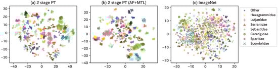
Figure A1.
Visualization of feature maps for each model using Perciformes images from the webfish-small dataset.
Figure A1.
Visualization of feature maps for each model using Perciformes images from the webfish-small dataset.
As a general trend, similar-appearing fish species were mapped close to each other in the latent space. In Figure A1b, Carangidae (•) with Scombridae (×) and Sparidae (⋆) with Lutjanidae (⧫) are placed close to each other in family. In terms of species, Trachurus japonicus and Decapterus maruadsi (of the Carangidae species) are placed close, while the groups to their left (Seriola quinqueradiata, Seriola dumerili, and Seriola lalandi) have very similar appearance. In addition, the two species on the right side of Scombridae (Scomber japonicus Houttuyn and Scomber australasicus Cuvier) and the left side of the Sparidae group (Pagrus major, Dentex hypselosomus Bleeker, and Evynnis tumifrons), as well as the two species of Other (Sphyraena pinguis Gunther and Sphyraena japonica Bloch and Schneider) in the lower center, have very similar appearances. (c) ImageNet indicates the distribution of feature maps outputted from ImageNet pre-trained model. The distribution of the various fish species is mixed, indicating that this is a latent space that does not take into account the similarity of the appearance of the fish. Thus, the model was able to steadily capture the similarity in the appearance of the fish species.
Figure A1a,b show the differences between models. In general, metric learning, such as AF Loss, was used to reduce the intraclass variance and increase the distance between classes. Although this is a qualitative assessment, it was observed, for example, in the Scombridae and Other species. The difference between the presence or absence of MTL is whether the loss function includes biological classifications. By including the biological classifications in the loss function, for example, in Figure A1a, the Serranidae were nearly placed into two groups (group 1: Plectropomus leopardus and Epinephelus akaara; group 2: Hyporthodus septemfasciatus, Epinephelus bruneus Bloch, and Niphon spinosus Cuvier), whereas, as shown in Figure A1b, they are placed closer together. Hexagrammidae, which were also placed far apart in (a), are placed relatively closer in (b). Thus, the latent space is constructed by using the AF Loss to accurately place the distance between fish species and the MTL to combine with the biological classifications.
In addition, determining whether a latent space based on the biological classifications defined by humans or a latent space obtained using end-to-end machine learning is better depends on the application. For example, although the latter model is less accurate in identifying fish species, it has potential for use in ichthyological research because it enables feature extraction based on appearance alone, without prior knowledge; this is more ideal during the discovery of new fish species.
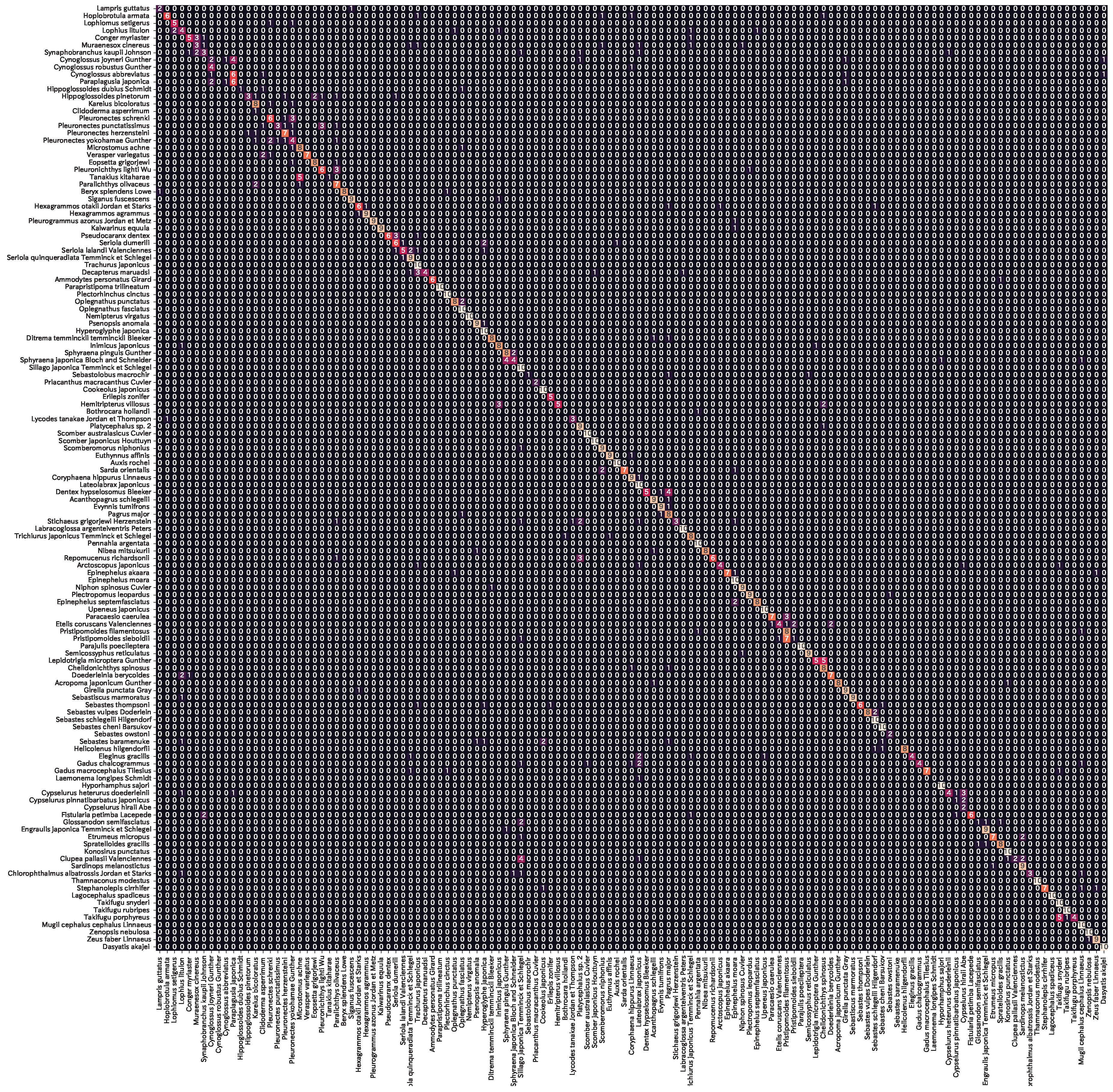
Appendix C. Confusion Matrices of Our Model
Figure A2 shows the confusion matrix of the prediction results for the output layer masking model (AF + MTL) of Swin_T, which achieved the highest accuracy. The accuracy of 72.9% indicates that the majority of the fish species were successfully classified. In terms of error patterns, Cynoglossidae, Pleuronectidae, Lutjanidae, and Exocoetidae tended to be misclassified within the same family. As error patterns were observed for fish species with similar appearance, the prediction is based on the similarity of appearance even when using the output layer masking.
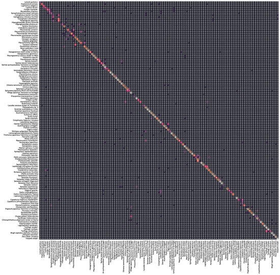
Figure A2.
Prediction results of Webfish-small dataset by output layer masking (Swin_T + AF + MLT).
Figure A2.
Prediction results of Webfish-small dataset by output layer masking (Swin_T + AF + MLT).
Notes
References
- Garcia, R.; Prados, R.; Quintana, J.; Tempelaar, A.; Gracias, N.; Rosen, S.; Vågstøl, H.; Løvall, K. Automatic segmentation of fish using deep learning with application to fish size measurement. ICES J. Mar. Sci. 2019, 77, 1354–1366. [Google Scholar] [CrossRef]
- Hasegawa, T.; Tanaka, M. Few-shot Fish Length Recognition by Mask R-CNN for Fisheries Resource Management. IPSJ Trans. Consum. Devices Syst. 2022, 12, 38–48. (In Japanese) [Google Scholar]
- Tseng, C.H.; Kuo, Y.F. Detecting and counting harvested fish and identifying fish types in electronic monitoring system videos using deep convolutional neural networks. ICES J. Mar. Sci. 2020, 77, 1367–1378. [Google Scholar] [CrossRef]
- Pornpanomchai, C.; Lurstwut, B.; Leerasakultham, P.; Kitiyanan, W. Shape- and Texture-Based Fish Image Recognition System. Agric. Nat. Resour. 2013, 47, 624–634. [Google Scholar]
- Rathi, D.; Jain, S.; Indu, S. Underwater Fish Species Classification using Convolutional Neural Network and Deep Learning. In Proceedings of the 2017 Ninth International Conference on Advances in Pattern Recognition (ICAPR), Bangalore, India, 27–30 December 2017; pp. 1–6. [Google Scholar] [CrossRef]
- Rauf, H.T.; Lali, M.I.U.; Zahoor, S.; Shah, S.Z.H.; Rehman, A.U.; Bukhari, S.A.C. Visual features based automated identification of fish species using deep convolutional neural networks. Comput. Electron. Agric. 2019, 167, 105075. [Google Scholar] [CrossRef]
- Deng, J.; Dong, W.; Socher, R.; Li, L.-J.; Li, K.; Li, F.-F. ImageNet: A large-scale hierarchical image database. In Proceedings of the 2009 IEEE Conference on Computer Vision and Pattern Recognition, Miami, FL, USA, 20–25 June 2009; pp. 248–255. [Google Scholar] [CrossRef]
- Allken, V.; Handegard, N.O.; Rosen, S.; Schreyeck, T.; Mahiout, T.; Malde, K. Fish species identification using a convolutional neural network trained on synthetic data. ICES J. Mar. Sci. 2018, 76, 342–349. [Google Scholar] [CrossRef]
- Mathur, M.; Goel, N. FishResNet: Automatic Fish Classification Approach in Underwater Scenario. SN Comput. Sci. 2021, 2, 273. [Google Scholar] [CrossRef]
- Murugaiyan, J.; Palaniappan, M.; Durairaj, T.; Muthukumar, V. Fish species recognition using transfer learning techniques. Int. J. Adv. Intell. Inform. 2021, 7, 188–197. [Google Scholar] [CrossRef]
- Ben Tamou, A.; Benzinou, A.; Nasreddine, K. Live Fish Species Classification in Underwater Images by Using Convolutional Neural Networks Based on Incremental Learning with Knowledge Distillation Loss. Mach. Learn. Knowl. Extr. 2022, 4, 753–767. [Google Scholar] [CrossRef]
- Zhou, Z.; Yang, X.; Ji, H.; Zhu, Z. Improving the classification accuracy of fishes and invertebrates using residual convolutional neural networks. ICES J. Mar. Sci. 2023, 80, 1256–1266. [Google Scholar] [CrossRef]
- Dey, K.; Bajaj, K.; Ramalakshmi, K.S.; Thomas, S.; Radhakrishna, S. FisHook—An Optimized Approach to Marine Species Classification using MobileNetV2. In Proceedings of the OCEANS 2023, Limerick, Ireland, 5–8 June 2023; pp. 1–7. [Google Scholar]
- Alaba, S.Y.; Nabi, M.M.; Shah, C.; Prior, J.; Campbell, M.D.; Wallace, F.; Ball, J.E.; Moorhead, R. Class-Aware Fish Species Recognition Using Deep Learning for an Imbalanced Dataset. Sensors 2022, 22, 8268. [Google Scholar] [CrossRef] [PubMed]
- Khan, F.F.; Li, X.; Temple, A.J.; Elhoseiny, M. FishNet: A Large-scale Dataset and Benchmark for Fish Recognition, Detection, and Functional Trait Prediction. In Proceedings of the 2023 IEEE/CVF International Conference on Computer Vision (ICCV), Paris, France, 1–6 October 2023; pp. 20439–20449. [Google Scholar]
- Boom, B.J.; Huang, P.X.; He, J.; Fisher, R.B. Supporting ground-truth annotation of image datasets using clustering. In Proceedings of the 21st International Conference on Pattern Recognition (ICPR2012), Tsukuba, Japan, 11–15 November 2012; pp. 1542–1545. [Google Scholar]
- LifeCLEF. LifeCLEF 2015 Fish Task. Available online: https://www.imageclef.org/lifeclef/2015/fish (accessed on 9 October 2023).
- Zhuang, P.; Wang, Y.; Qiao, Y. WildFish: A Large Benchmark for Fish Recognition in the Wild. In Proceedings of the 2018 ACM Multimedia Conference on Multimedia Conference, Seoul, Republic of Korea, 22–26 October 2018; pp. 1301–1309. [Google Scholar]
- Zhuang, P.; Wang, Y.; Qiao, Y. Wildfish++: A Comprehensive Fish Benchmark for Multimedia Research. IEEE Trans. Multimed. 2021, 23, 3603–3617. [Google Scholar] [CrossRef]
- Shah, S.Z.H.; Rauf, H.T.; IkramUllah, M.; Khalid, M.S.; Farooq, M.; Fatima, M.; Bukhari, S.A.C. Fish-Pak: Fish species dataset from Pakistan for visual features based classification. Data Brief 2019, 27, 104565. [Google Scholar] [CrossRef] [PubMed]
- Ulucan, O.; Karakaya, D.; Turkan, M. A Large-Scale Dataset for Fish Segmentation and Classification. In Proceedings of the 2020 Innovations in Intelligent Systems and Applications Conference (ASYU), Istanbul, Turkey, 15–17 October 2020; pp. 1–5. [Google Scholar]
- Liu, C.; Li, H.; Wang, S.; Zhu, M.; Wang, D.; Fan, X.; Wang, Z. A Dataset and Benchmark of Underwater Object Detection for Robot Picking. In Proceedings of the 2021 IEEE International Conference on Multimedia & Expo Workshops (ICMEW), Shenzhen, China, 5–9 July 2021; pp. 1–6. [Google Scholar]
- Garcia-d’Urso, N.; Galan-Cuenca, A.; Pérez-Sánchez, P.; Climent-Pérez, P.; Fuster-Guillo, A.; Azorin-Lopez, J.; Saval-Calvo, M.; Guillén-Nieto, J.E.; Soler-Capdepón, G. The DeepFish computer vision dataset for fish instance segmentation, classification, and size estimation. Sci. Data 2022, 9, 287. [Google Scholar] [CrossRef]
- Boulais, O.E.; Alaba, S.Y.; Yu, J.; Iftekhar, A.T.; Zheng, A.; Prior, J.; Moorhead, R.; Ball, J.; Primrose, J.; Wallace, F. SEAMAPD21: A large-scale reef fish dataset for fine-grained categorization. In Proceedings of the FGVC8: The Eight Workshop on Fine-Grained Visual Categorization CVPR 2021, Online, 25 June 2021. [Google Scholar]
- Ou, L.; Liu, B.; Chen, X.; He, Q.; Qian, W.; Zou, L. Automated Identification of Morphological Characteristics of Three Thunnus Species Based on Different Machine Learning Algorithms. Fishes 2023, 8, 182. [Google Scholar] [CrossRef]
- Suzuki, A.; Sakanashi, H.; Kido, S.; Shouno, H. Feature Representation Analysis of Deep Convolutional Neural Network using Two-stage Feature Transfer—An Application for Diffuse Lung Disease Classification. IPSJ Trans. Math. Model. Its Appl. 2018, 11, 74–83. [Google Scholar]
- Dana, K.J.; van Ginneken, B.; Nayar, S.K.; Koenderink, J.J. Reflectance and Texture of Real-World Surfaces. Acm Trans. Graph. 1999, 18, 1–34. [Google Scholar] [CrossRef]
- Zhang, X.; Chen, Z.; Gao, J.; Huang, W.; Li, P.; Zhang, J. A two-stage deep transfer learning model and its application for medical image processing in Traditional Chinese Medicine. Knowl.-Based Syst. 2022, 239, 108060. [Google Scholar] [CrossRef]
- Zhang, W.; Deng, L.; Zhang, L.; Wu, D. A Survey on Negative Transfer. IEEE/CAA J. Autom. Sin. 2023, 10, 305–329. [Google Scholar] [CrossRef]
- Soviany, P.; Ionescu, R.T.; Rota, P.; Sebe, N. Curriculum Learning: A Survey. Int. J. Comput. Vis. 2022, 130, 1526–1565. [Google Scholar] [CrossRef]
- Shen, X.; Wang, Y.; Lin, M.; Huang, Y.; Tang, H.; Sun, X.; Wang, Y. DeepMAD: Mathematical Architecture Design for Deep Convolutional Neural Network. In Proceedings of the IEEE/CVF Conference on Computer Vision and Pattern Recognition (CVPR), Vancouver, BC, Canada, 17–24 June 2023; pp. 6163–6173. [Google Scholar]
- Chen, X.; Liang, C.; Huang, D.; Real, E.; Wang, K.; Liu, Y.; Pham, H.; Dong, X.; Luong, T.; Hsieh, C.J.; et al. Symbolic Discovery of Optimization Algorithms. arXiv 2023, arXiv:2302.06675. [Google Scholar]
- Radford, A.; Kim, J.W.; Hallacy, C.; Ramesh, A.; Goh, G.; Agarwal, S.; Sastry, G.; Askell, A.; Mishkin, P.; Clark, J.; et al. Learning Transferable Visual Models from Natural Language Supervision. In Proceedings of the 38th International Conference on Machine Learning, Virtual, 18–24 July 2021; Volume 139, pp. 8748–8763. [Google Scholar]
- He, K.; Zhang, X.; Ren, S.; Sun, J. Deep Residual Learning for Image Recognition. In Proceedings of the 2016 IEEE Conference on Computer Vision and Pattern Recognition (CVPR), Las Vegas, NV, USA, 27–30 June 2016; pp. 770–778. [Google Scholar] [CrossRef]
- Liu, Z.; Lin, Y.; Cao, Y.; Hu, H.; Wei, Y.; Zhang, Z.; Lin, S.; Guo, B. Swin Transformer: Hierarchical Vision Transformer Using Shifted Windows. In Proceedings of the IEEE/CVF International Conference on Computer Vision (ICCV), Montreal, BC, Canada, 11–17 October 2021; pp. 10012–10022. [Google Scholar]
- Cubuk, E.D.; Zoph, B.; Shlens, J.; Le, Q. RandAugment: Practical Automated Data Augmentation with a Reduced Search Space. In Advances in Neural Information Processing Systems; Larochelle, H., Ranzato, M., Hadsell, R., Balcan, M., Lin, H., Eds.; Curran Associates, Inc.: Nice, France, 2020; Volume 33, pp. 18613–18624. [Google Scholar]
- Loshchilov, I.; Hutter, F. SGDR: Stochastic Gradient Descent with Warm Restarts. In Proceedings of the International Conference on Learning Representations, Toulon, France, 24–26 April 2017. [Google Scholar]
- Szegedy, C.; Vanhoucke, V.; Ioffe, S.; Shlens, J.; Wojna, Z. Rethinking the Inception Architecture for Computer Vision. In Proceedings of the 2016 IEEE Conference on Computer Vision and Pattern Recognition (CVPR), Las Vegas, NV, USA, 27–30 June 2016; pp. 2818–2826. [Google Scholar] [CrossRef]
- Zhang, Y.; Yang, Q. An overview of multi-task learning. Natl. Sci. Rev. 2017, 5, 30–43. [Google Scholar] [CrossRef]
- Deng, J.; Guo, J.; Xue, N.; Zafeiriou, S. ArcFace: Additive Angular Margin Loss for Deep Face Recognition. In Proceedings of the 2019 IEEE/CVF Conference on Computer Vision and Pattern Recognition (CVPR), Long Beach, CA, USA, 15–20 June 2019; pp. 4685–4694. [Google Scholar] [CrossRef]
- Dhall, A.; Makarova, A.; Ganea, O.; Pavllo, D.; Greeff, M.; Krause, A. Hierarchical Image Classification using Entailment Cone Embeddings. In Proceedings of the 2020 IEEE/CVF Conference on Computer Vision and Pattern Recognition Workshops (CVPRW), Seattle, WA, USA, 14–19 June 2020; pp. 3649–3658. [Google Scholar] [CrossRef]
- Chen, Y.; Zhu, G. Using machine learning to alleviate the allometric effect in otolith shape-based species discrimination: The role of a triplet loss function. ICES J. Mar. Sci. 2023, 80, 1277–1290. [Google Scholar] [CrossRef]
- Yang, Z.; Li, J.; Chen, T.; Pu, Y.; Feng, Z. Contrastive learning-based image retrieval for automatic recognition of in situ marine plankton images. ICES J. Mar. Sci. 2022, 79, 2643–2655. [Google Scholar] [CrossRef]
- Tan, M.; Le, Q. EfficientNet: Rethinking Model Scaling for Convolutional Neural Networks. In Proceedings of the 36th International Conference on Machine Learning, Long Beach, CA, USA, 9–15 June 2019; Chaudhuri, K., Salakhutdinov, R., Eds.; Volume 97, pp. 6105–6114. [Google Scholar]
- Tan, M.; Le, Q. EfficientNetV2: Smaller Models and Faster Training. In Proceedings of the 38th International Conference on Machine Learning, Virtual, 18–24 July 2021; Meila, M., Zhang, T., Eds.; Volume 139, pp. 10096–10106. [Google Scholar]
- Xu, J.; Pan, Y.; Pan, X.; Hoi, S.; Yi, Z.; Xu, Z. RegNet: Self-Regulated Network for Image Classification. IEEE Trans. Neural Netw. Learn. Syst. 2022, 34, 1–6. [Google Scholar] [CrossRef]
- Liu, Z.; Mao, H.; Wu, C.Y.; Feichtenhofer, C.; Darrell, T.; Xie, S. A ConvNet for the 2020s. In Proceedings of the 2022 IEEE/CVF Conference on Computer Vision and Pattern Recognition (CVPR), New Orleans, LA, USA, 18–24 June 2022; pp. 11966–11976. [Google Scholar] [CrossRef]
- Bommasani, R.; Hudson, D.A.; Adeli, E.; Altman, R.; Arora, S.; von Arx, S.; Bernstein, M.S.; Bohg, J.; Bosselut, A.; Brunskill, E.; et al. On the Opportunities and Risks of Foundation Models. arXiv 2021, arXiv:2108.07258. [Google Scholar]
- Tanaka, M.; Hasegawa, T. Explainable Few-Shot fish classification method using CLIP. In Proceedings of the 85th National Convention of IPSJ, Tokyo, Japan, 2–4 March 2023; Volume 2023. (In Japanese). [Google Scholar]
- van der Maaten, L.; Hinton, G. Visualizing Data using t-SNE. J. Mach. Learn. Res. 2008, 9, 2579–2605. [Google Scholar]


Disclaimer/Publisher’s Note: The statements, opinions and data contained in all publications are solely those of the individual author(s) and contributor(s) and not of MDPI and/or the editor(s). MDPI and/or the editor(s) disclaim responsibility for any injury to people or property resulting from any ideas, methods, instructions or products referred to in the content. |
© 2024 by the authors. Licensee MDPI, Basel, Switzerland. This article is an open access article distributed under the terms and conditions of the Creative Commons Attribution (CC BY) license (https://creativecommons.org/licenses/by/4.0/).