Abstract
With the development of bridge crossings over rivers, the accident of the vessel–bridge collision is increasing as well. It is important to assess probability of bridges colliding with passing ships. Firstly, the AIS (Automatic identify system) data was collected and decoded to obtain the dynamic information of the ships passing the bridge including the distributions of ships position, speed, and yaw angle, which are then compared with the value recommended by the AASHTO (American Association of State Highway and Transportation Officials) specification. The mainly influential parameters of ship–bridge collision obtained from AIS data are used to correct the variables in the risk assessment of AASHTO specification, which intends to improve the assessment accuracy by considering the actual information of passing vessels. The collision probability with and without considering the actual situations of passing ships are compared. It is found that the distribution and transit path of passing ships significantly influence the collision probability. To improve the risk assessment accuracy, it is suggested to use the actual distributions of passing ships from AIS data.
1. Introduction
With increasing transportation, more bridges crossing rivers have been built, which could be artificial obstacles in the channel of ships [1] and would increase the allision risk between ship and bridge. Although several rules are required to comply for reducing the risk associated with collision during the bridge design stage, many kinds of reason still could cause ship impact accident, which is impossible to avoid completely [2]. In 2007, a general cargo ship impacted the pier of Jiujiang Bridge and caused a collapse in Guangdong Province, China, as shown in Figure 1 [3].
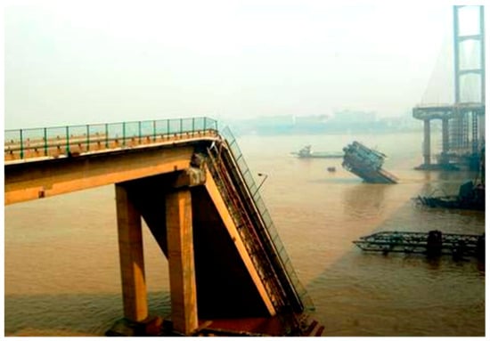
Figure 1.
Collapse of Jiujiang Bridge under errant ship impact in Guangdong Province, China (2007).
Gholipour and Zhang [4] investigated the progressive damage behaviours and nonlinear failure modes of a cable-stayed bridge pier subjected to ship collisions using finite element (FE) simulations. An analytical simplified model with two-degree-of-freedom (2-DOF) was proposed to formulate the strain rate effects of the concrete materials as the dynamic increase factors in the global responses of the impacted pier. However, the impact accident between the ship and bridge is an occasional event. It is necessary to use risk analysis to assess the actual the safety level of bridge against ship collision. The probability of a collision accident can be assessed by the historical data, expert opinions, and predictive calculations [5]. The statistical method uses the existing accident data of ship–bridge collision to predict the allision probability of ship–bridge. The statistical method is reasonable, but it needs a lot of accident data that might be absent and is not practical. There exists very few relevant statistical data for the ship–bridge allision accident, since that is a small probability event or even does not occur for a newly designed bridge. Hence, the statistical method is limited to some extent for the assessment of allision risk between the ship and bridge.
The mathematical models for predicting frequency of the collision occurrence are an important first step in the risk assessment of bridge against ship allision. The method of probabilistic analyses should consider the scenario of actual passing ships. Based on the occurrence mechanism of ship–bridge allision accident, Kunz [6] studied the failure trajectory of aberrancy ship and the collision probability of ship–bridge, which provided a risk analysis method and procedure. Pedersen et al. [7,8] presented a basis for the estimation of collision forces between conventional merchant vessels and large-volume offshore structures in the form of bridges crossing international shipping routes and gravity-supported offshore installations. The crushing forces are determined as functions of vessel size, vessel speed, bow profile, collision angles and eccentric impacts.
The collision probability was quantitatively evaluated according to the maritime traffic distribution by Lee [9] and Son and Cho [10] according to the AASHTO (American Association of State Highway and Transportation Officials) requirement [11]. The corresponding results showed that the annual collision frequency of once every 50–100 years was suitable depending on the ship size. In the risk analysis of ship collisions, it is very important to obtain the distributions of the speed, position, and angle of passing ship during a certain time period. However, due to the limitation of data collection conditions, the values of relevant parameters in the requirement might be different from the actual scenarios. The application of AIS data makes it possible to investigate accurate and actual behavior of collision-involved ships, and benefits vessel traffic management and waterways design for special areas [12,13]. Hansen et al. [14] carried out ship collision risk studies for different bridge designs for the Sognefjorden Strait, which demonstrated that the use of AIS data forms a solid basis for establishing a ship collision risk model that can evaluate ship collision frequencies. Zeman [15,16] used the AIS data in Japan and Malaysia to establish the risk identification and evaluation model by fuzzy mathematics method. Xiao et al. [17] also adopted AIS data to characterize the lateral position, speed, heading direction for different types and sizes of ships, and then compared the ship traffic characteristics between the Netherlands and the Yangtze River in China, which shows that the distributions of ship characteristics differ significantly in various waterways. Wu et al. [18] used AIS data to study the travel behavior of vessels when passing through a hotspot in a narrow waterway. The findings reveal the travel patterns of inbound and outbound trips passing these three hotspots in the SNWW (Sabine–Neches Waterways), and more than 10% of total vessel conflicts occurred within these three hotspots. Fiorini et al. [19] conducted a related study on the spatial planning of ship traffic flow by analyzing ship AIS data.
Horteborn and Ringsberg [20] presented a methodology that uses AIS data and a ship maneuvering simulator to simulate and analyze marine traffic schemes regarding accidents risks. The historical multi-ship encounter scenarios involved ferries from AIS data. The values of RIFs (Risk Influencing Factors) between ships were calculated according to their cumulative distribution, and their corresponding weights are determined using entropy theory [21]. Cauteruccio et al. [22] propose a framework that aims at handling metrics among strings defined over heterogeneous alphabet.
The AASHTO specification [11] provides a convenient procedure to assess the collision risk between ship and bridge, in which the relevant parameters are assumed based on the historical statistical data from the information in the USA. However, the recommended variables might be different from the actual situation, and thus the results of risk analysis in the AASHTO specification cannot reflect the actual situation.
The purpose of present paper is to figure out a method that is easy to carry out and could reflect the actual scenarios. Based on the AIS data of ships passing Tongling Bridge of Yangtze River, the distributions of type, tonnage, speed, and yaw angle of the passing ship are investigated first. To consider the actual situation, the variables in the risk assessment method of the AASHTO specifications [10] are corrected by statistical analysis of AIS data, and then the allision probability between ship and bridge is investigated as well.
2. Statistical Analysis of Traffic Flow of Ships
2.1. Bridge Condition and AIS Data Collection
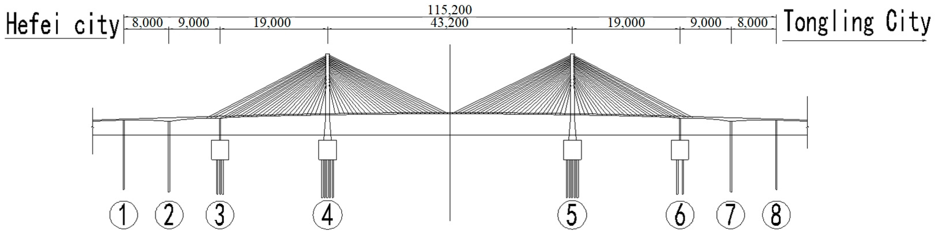
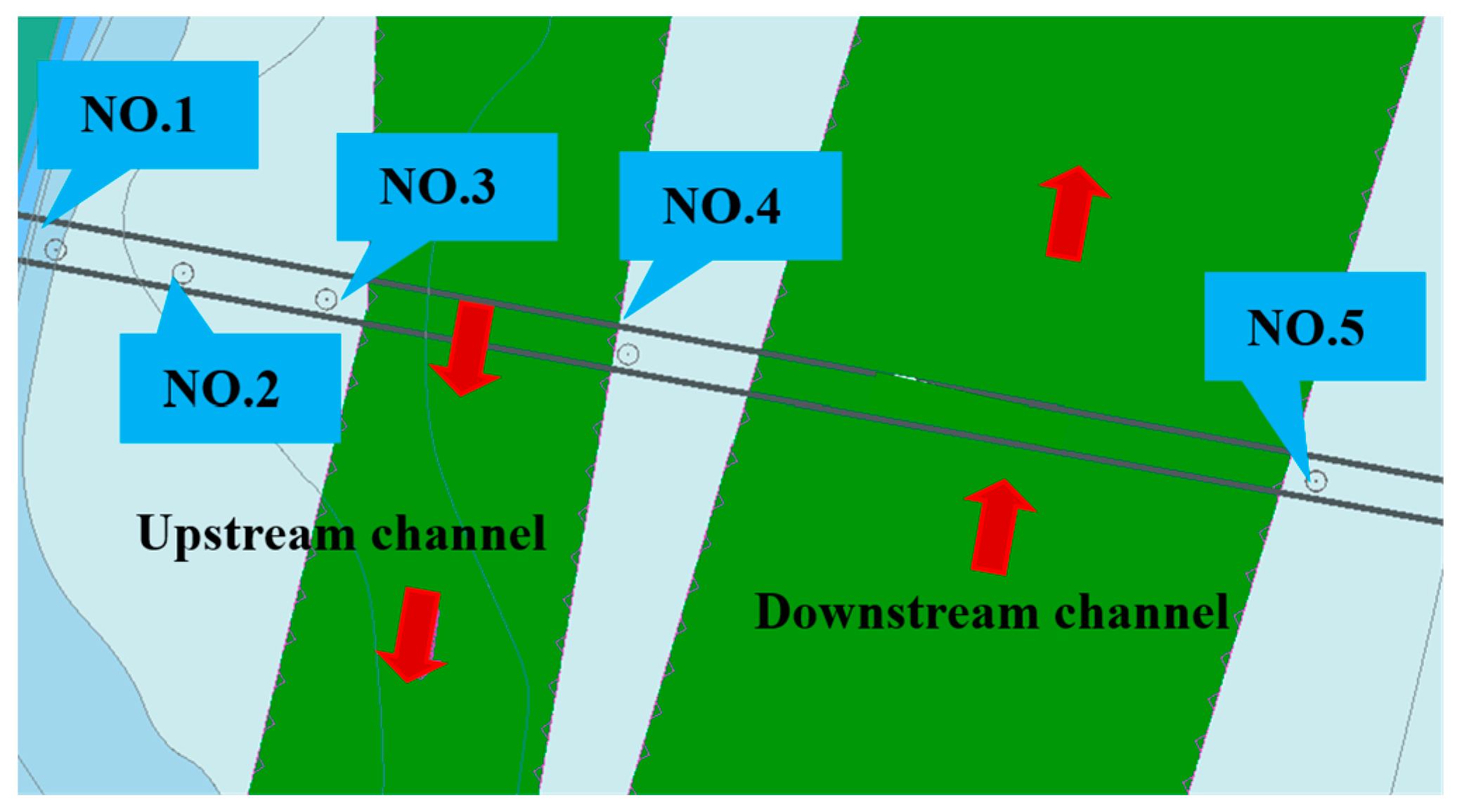
The total length of Tongling Bridge crossing Yangtze River is 2592 m, and the corresponding span arrangement is 80 + 90 + 190+ 432 + 190 + 90 + 80 m as shown in Figure 2. The piers number of bridge from Hefei to Tongling city are from NO.1 to NO.8. The upstream channel is between NO.3 and NO.4, and the downstream channel is between the two main tower piers NO.4 and NO.5 as shown in Figure 3, respectively.
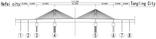
Figure 2.
Tongling Bridge of Yangtze River (Unit: cm, ① to ⑧ means the piers number).
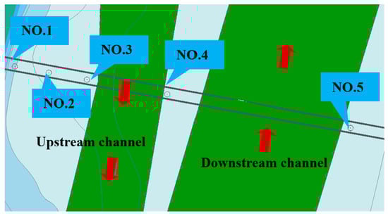
Figure 3.
Arrangement of bridge piers and traffic flow channels (The red arrow means the direction of ship passing under bridge).
The accuracy of ship collision risk significantly relies on several variables, including the layout of navigable channel, the traffic flow and characteristics of ships passing bridge. Using high frequency information, AIS data is transmitted from ships to ashore. The frequent interval of sending information is approximately 3–10 s, which make it possible to track every passing ship and then provide influential parameters for the risk analysis of ship and bridge collision. According to international SOLAS requirement [12] since 2002, AIS equipment have been required to install on the ships with larger 300 t displacement and all passenger ships, which make it possible to collect most information of ships that could be used in the risk analysis. The AIS data includes the principal dimensions, position, heading direction and speed of passing ships, which provides a flexible and comprehensive method to provide the statistical data for ship traffic flow. AIS equipment was set up near the bridge to collect the signal of passing ships and decoded for obtaining mainly information of ships passing the Tongling Bridge of Yangtze River.
2.2. Traffic Flow of Passing Ships
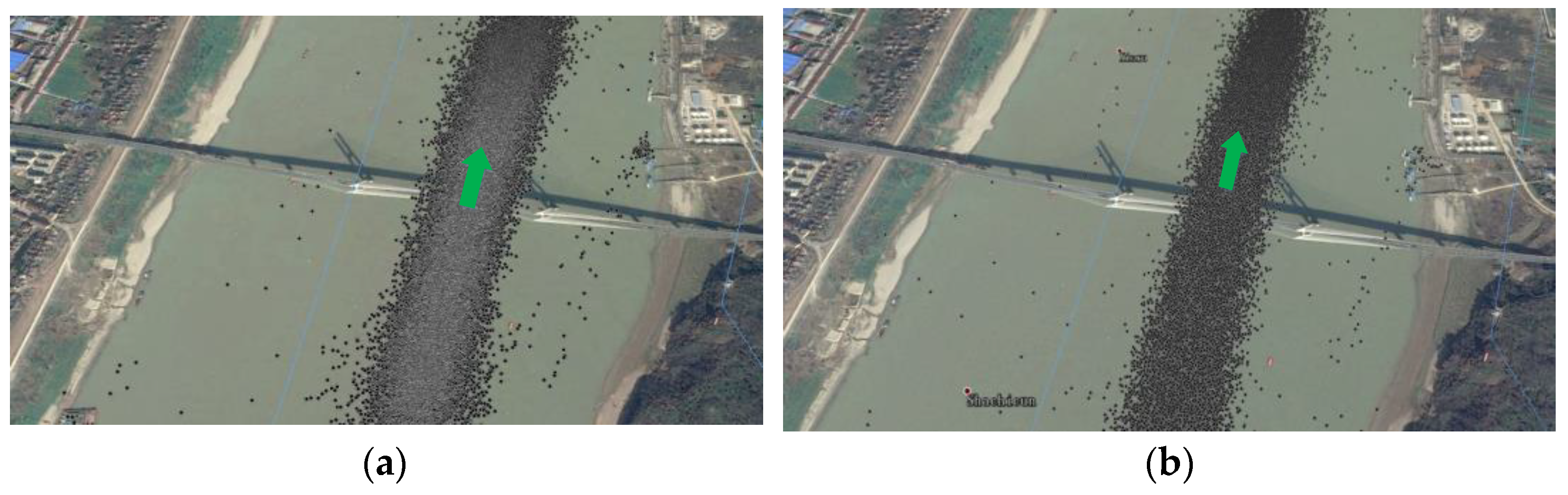
The information of ships passing the bridge were collected during March 2013 and March 2016 based on AIS data. The water level could influence the navigation behaviors of ships. Moreover, since the speed of water flow and water level in tide period are generally higher than that in the dry season, it necessary to discuss the ship traffic in different periods separately. The traffic flows of the passing ships in different periods are shown in Figure 4 and Figure 5, in which the green arrow presents the navigation direction. The flood season period is set as between June and September, and the low water period is set as during October and May of the following year. The green arrows present the navigation direction of ships passing under bridge in Figure 4 and Figure 5.

Figure 4.
Traffic flow of downstream ships: (a) During flood season period; (b) During low water period.
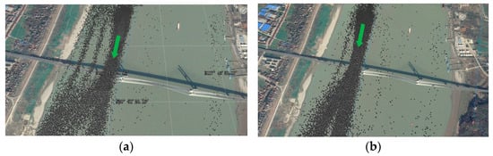
Figure 5.
Traffic flow of upstream ships: (a) During flood season period; (b) During low water period.
Since the navigable area for ships during flood season period with high water level is wider than that during low water period, the traffic flows of passing ships varies in different periods as expected, especially for the upstream ships. The transit paths and distribution of the downstream ships are similar during both the flood season period and the low water period in Figure 4, because of the water between piers NO.4 and NO.5 of the designed navigation channel is deep enough to pass for most of the downstream ships. However, the vessel transit path during the flood season period is slightly wider than that during the low water period.
For upstream ships, the distribution of traffic flow during the flood season period is more scattered than that during the low water period in Figure 5. During the low water period, the traffic flow of the upstream ships is close to the designed channel between piers NO.3 and NO.4. During the flood season period with high water levels, although most of the upstream ships navigates the designed channel between piers NO.3 and NO.4, some of them passed nearby piers NO.1 and NO.2. Some upstream ships do not follow the traffic rules, which is not expected and then would increase probability of ships colliding with the piers NO.1 and NO.2 during the flood season period. This phenomenon should be considered in the assessment of allision risk between ship and bridge.
2.3. Statistic Analysis of Passing Ships
The cubic spline interpolation with 10 s-interval is adopted for data synchronization regarding ship position (longitude and latitude), ship speed and heading. According to protocol ITU-RM.1371, the information decoded from AIS data includes the length, breadth and draught, velocity, yaw angle, and type of passing ships, which are important parameters in the risk assessment of ship–bridge collision.
Table 1 shows the number of various types of ships passing under bridge between March 2013 and March 2016. The average number of passing ships per day is 1019. Most of the ships passing the bridge (around 90%) are general cargo ships. The proportions of the containers and bulk carriers are both close to 5%. Hence, the general cargo ship could be assumed as the principal ship type in the anti-collision analysis of the bridge.

Table 1.
Number of passing ships.
- Distributions of ship dimensions
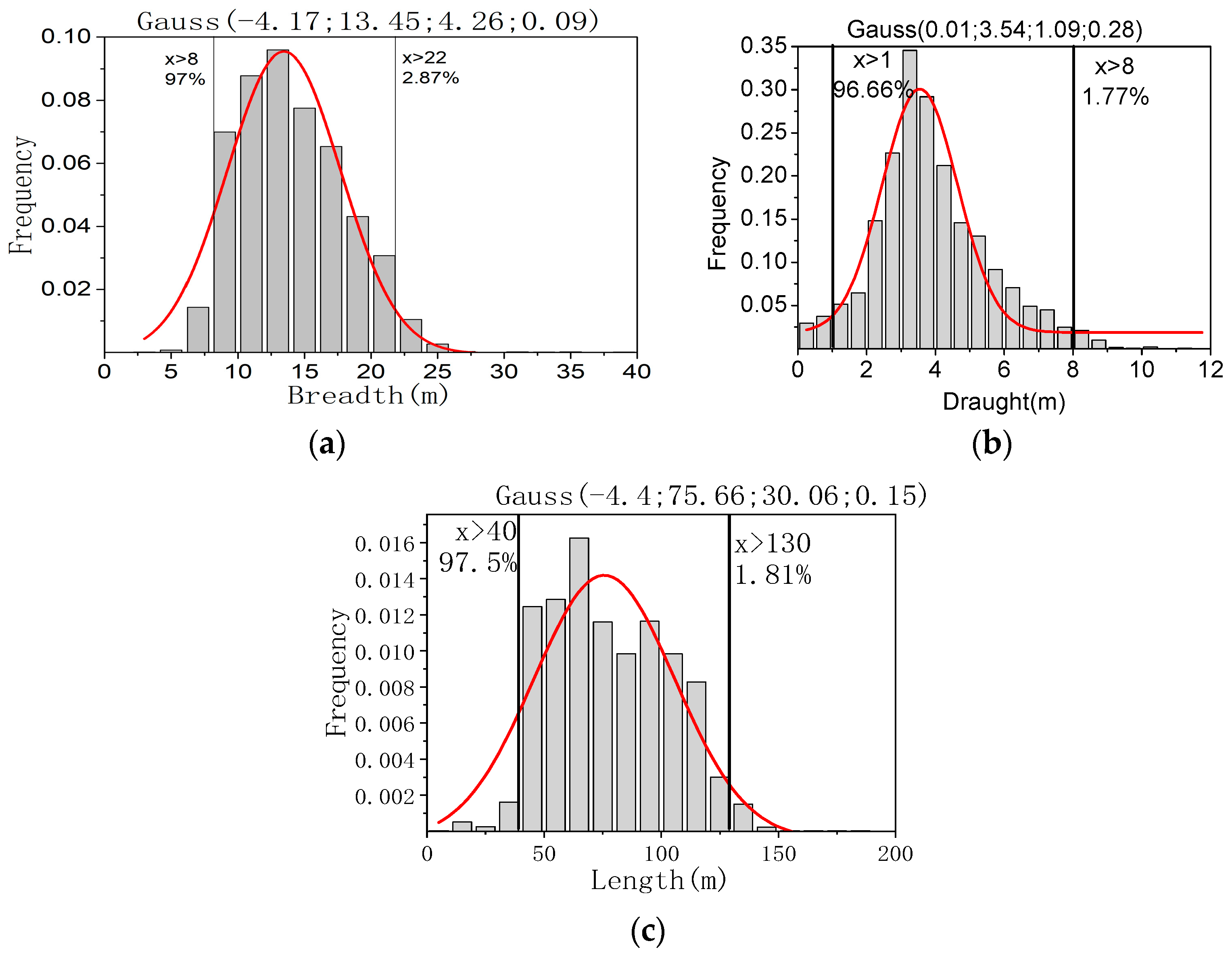
The distributions of length, breadth, and draught of passing ships obtained from AIS data collected from March 2013 to March 2016 are shown in Figure 6. According to the statistical analysis, the mean value of length, breadth, and draught of passing ships are 78.1 m, 13.3 m, and 3.8 m. As for 95% of ships, the dimensional ranges are between 40 m and 130 m for length, between 8 and 25 m for breadth, and between 1 m and 8 m for draught.
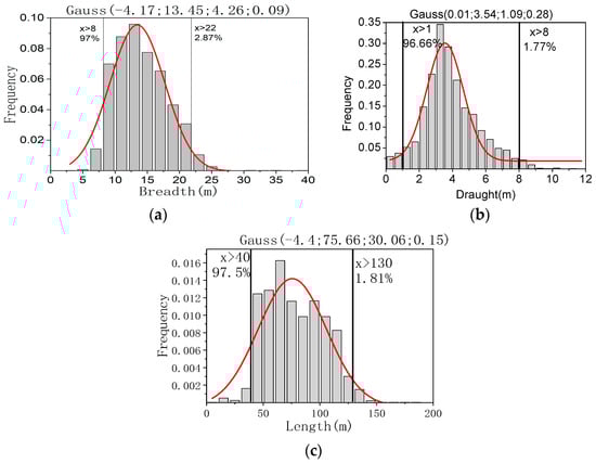
Figure 6.
Dimensional distributions of passing ships: (a) Distribution of length; (b) Distribution of breadth; (c) Distribution of draught.
From the observation of the distributions in Figure 6 and the statistical data, the distribution of ship principal dimensions is assumed as Gauss distribution, and the expression of the regression equation is given as follows.
where y0, xc, w, a are the fitting parameters in the Gauss distribution function and x is the independent variable.
The regression equations are expressed by.
The approximating accuracy of the regression function can be estimated by the coefficient of multiple determinations, which is statistical data that give the measurement of the correlation between the referential results and the assessment of the regression function and is given by following expression.
where
R: coefficient of determination
: total number of samples
: value of sample
y: theoretical value calculated by the regression equation
The coefficients of determination of regression function are 0.858, 0.955, and 0.933 for length, breadth, and draught in Table 2, respectively. The distributions of regression formulae for breadth and draught are very close to the statistical data (see Figure 6b,c), which illustrates that the regression equation is in good agreement with the measured data. The value of R for ship length is 0.858, which means that the fitting accuracy is not very good, which also can be observed in Figure 6a.
Table 2.
The distributions of ship principal dimensions.
The displacement weight of the ships passing the bridge is also an important parameter in the risk assessment of bridge safety. For vessels transiting in other than a fully loaded condition, the displacement weight can be estimated by following formula [11].
where
W: displacement weight of vessel
Cb: block coefficient (dimensionless)
Lw: length of vessel waterline
DM: mean draft of ship
BM: mean breadth of ships
Ww: 34.4 for saltwater, and 35.4 for freshwater
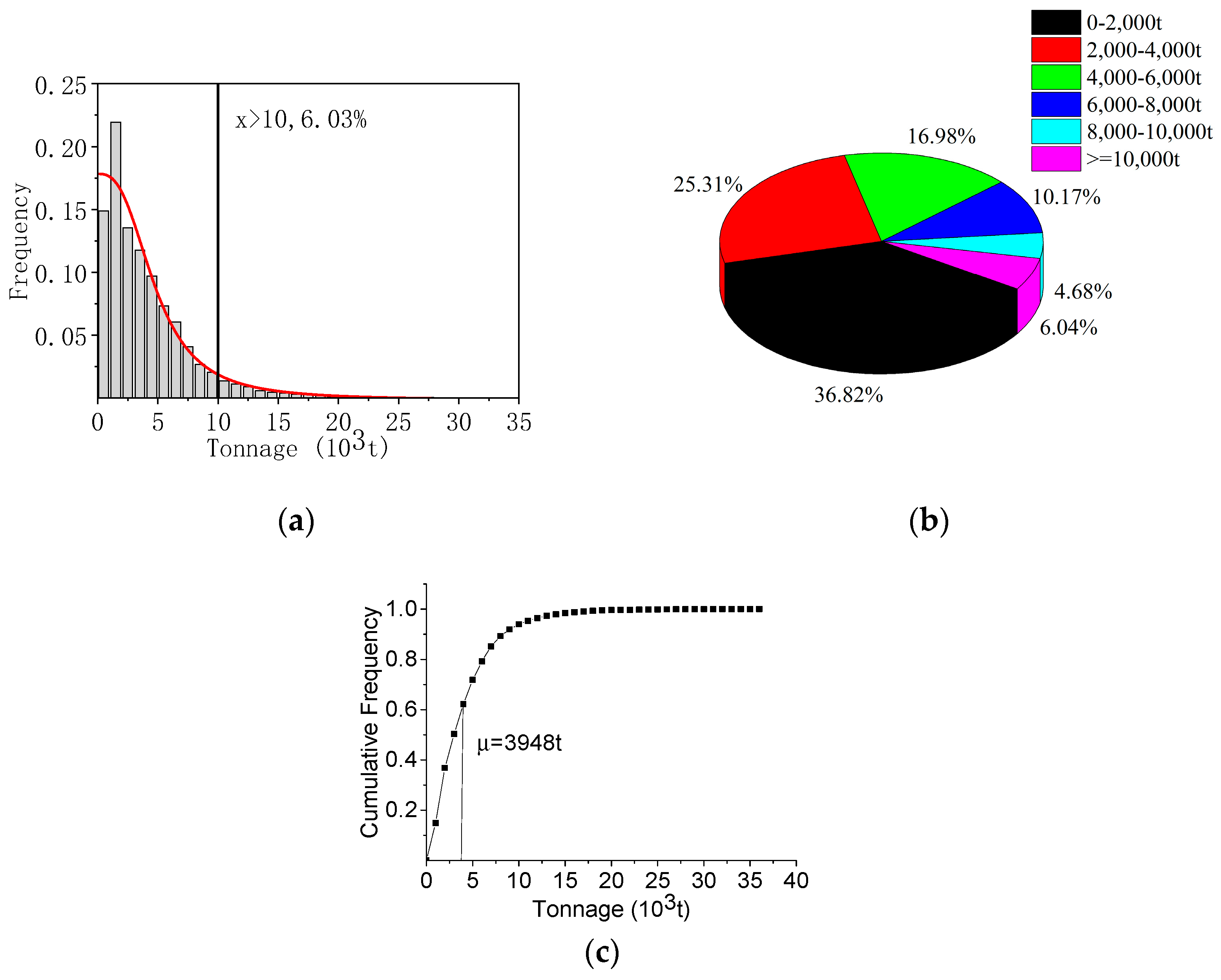
The statistical results of ship displacement weight are plotted in Figure 7. From the statistical data, the mean displacement weight of the ships passing under bridge is 3948 t, and 94% ships are smaller than 10,000 t. The maximum displacement weight of the ships is around 20,000 t.
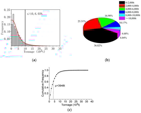
Figure 7.
Statistical results of ship displacement weight: (a) Distribution; (b) Proportion; (c) Cumulative frequency.
The accuracy of regression also depends on the assumed expression. Hence, three formulae are used to regress the distribution of ships displacement, which includes Gauss distribution with Equation (1), Gumbel distribution and Logistic distribution that are expressed as follows.
For Gumbel distribution:
where a, u are the fitting parameters, and x is the independent parameter.
For Logistic distribution:
where , p are the fitting parameters, and x is the independent parameter.
Figure 7 shows the statistical results of ship displacement. The coefficients of determination of regression function are 0.831, 0.911 and 0.959 for Gauss, Gumbel and Logistic functions in Table 3, respectively, which means that the Logistic distributions are more suitable to fitting the ship displacement than that of Gauss and Gumbel functions. The regression equation using Logistic distribution for ship displacement weight is given as follows.
Table 3.
The distributions of ship displacement weight.
- Distribution of velocity
The speed, weight, and heading direction of the passing ship are important factors in risk analysis of the ship–bridge collision, which determines the collision energy of ships. From the view of marine traffic engineering, the distribution and average of a ship’s speed passing through a certain water area or channel are of more concern. The average speed of the ship relative to ground is calculated by the following expression.
where Vi is the speed of ship i; ni is the number of AIS data sent by ship i; and SOGij means the speed to ground for ship i at the moment j decoded from AIS data.
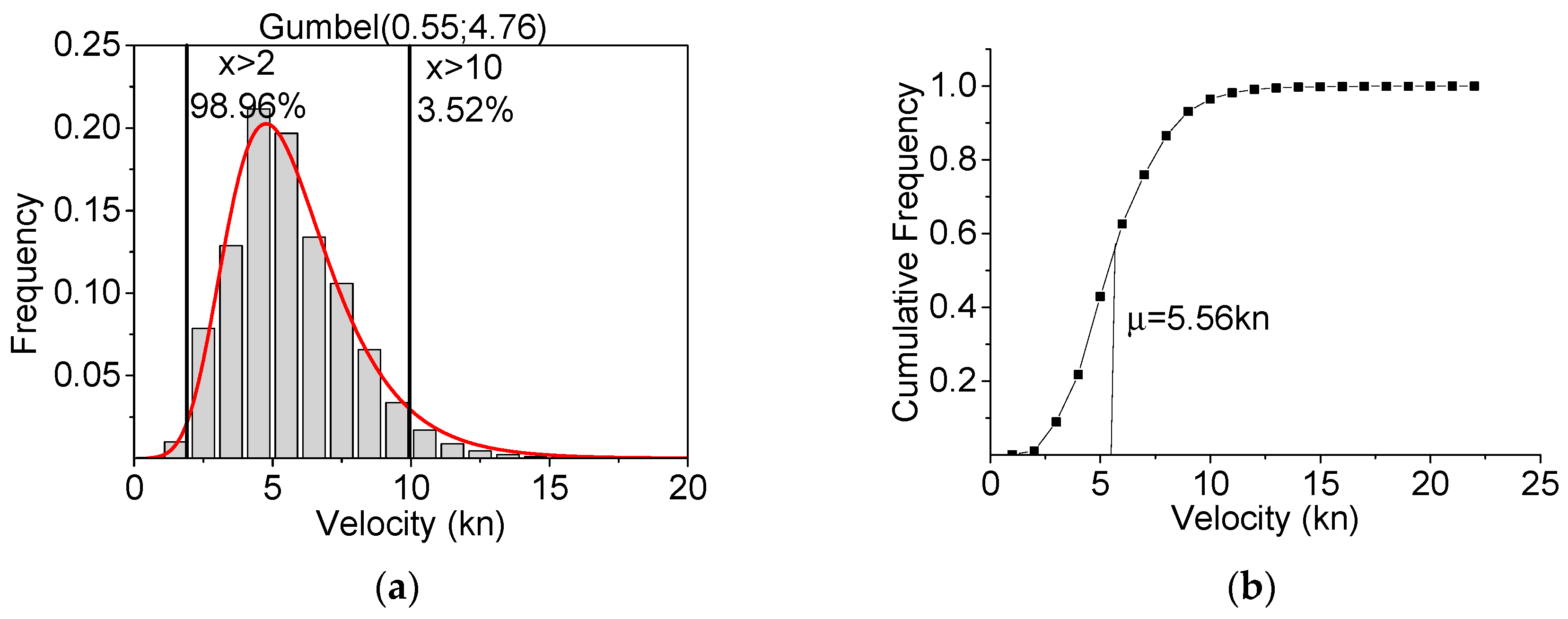
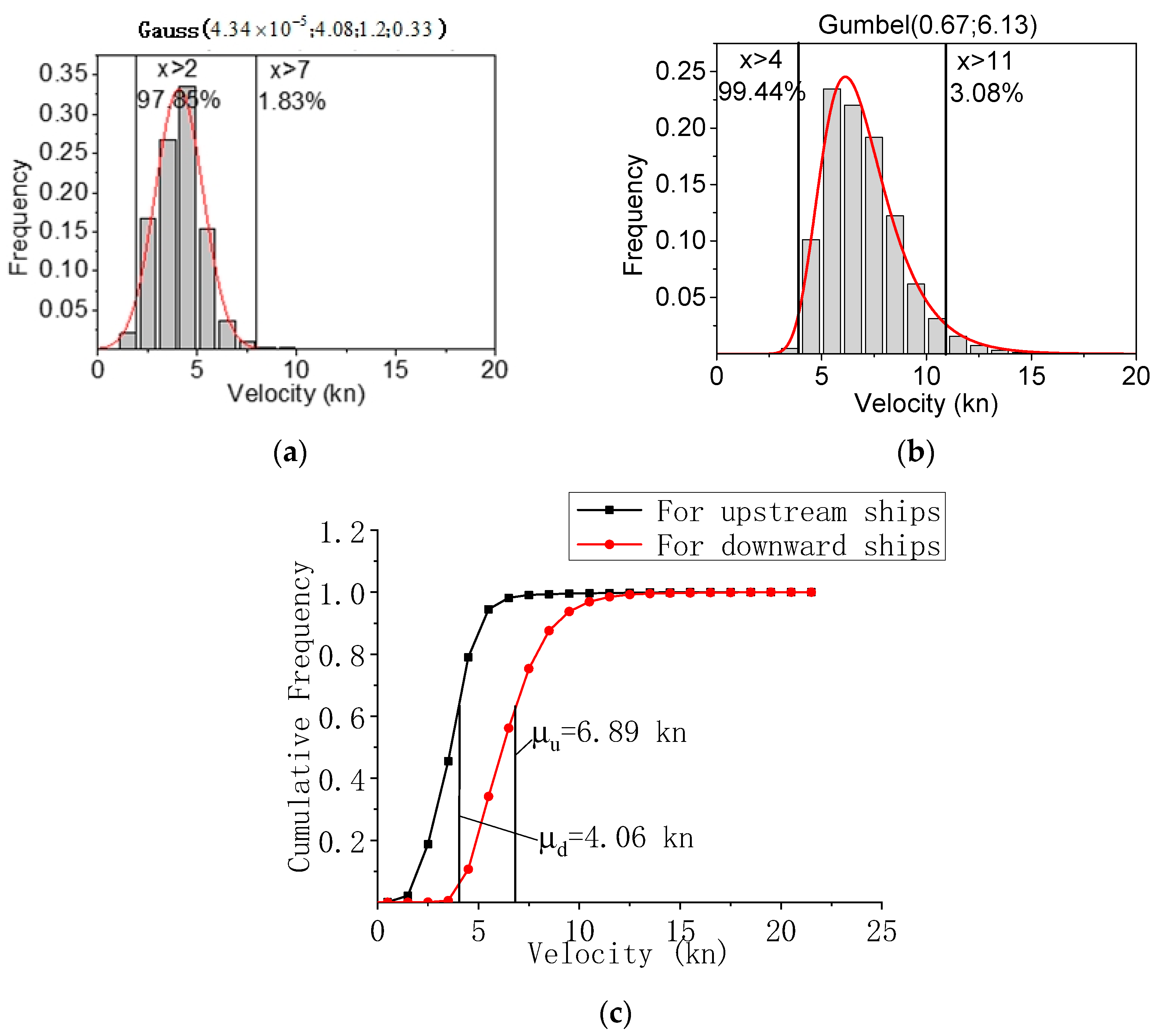
The statistical results of the ships’ velocity are shown in Figure 8. The maximum velocity of ship is 15 kn., 95% of the ships’ speed are less than 10 kn and the mean velocity is about 5.56 kn. The velocities in upstream and downstream channels are shown in Figure 9. The mean velocities of the downstream and upstream ships are 6.89 kn and 4.06 kn, respectively.

Figure 8.
Statistical results of ship velocity: (a) Frequency; (b) Cumulative frequency.
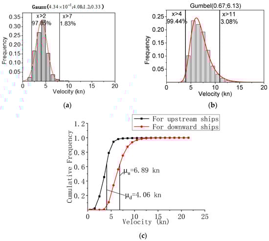
Figure 9.
Statistical results of ship velocity in both upstream and downstream channels: (a) For upstream ships; (b) For downstream ships; (c) Cumulative frequency of velocity.
The mean velocities for 99% of ships are less than 8 kn and 13 kn in upstream and downstream channels, respectively. The water flow has a great impact on the speed of passing ships, which causes that the velocity for upstream and downstream ships are very different and should be considered separately in the risk analysis of bridge anti-collision.
The Gauss and Gumbel distributions are both used to regress the ship velocities, expressed as follows.
For upstream ships with Gauss distribution:
For downstream ship with Gumbel distribution:
Velocity for both upstream and downstream ships with Gumbel distribution:
The distributions of ship velocity are given in Table 4. The minimum coefficient of determination using Gauss and Gumbel distributions is 9.48, which illustrates that the two type distributions can both regress the velocity well, but they are slightly different. It seems that the Gumbel distribution is more suitable for regressing ship velocity.
Table 4.
The distributions of ship velocity.
- Distribution of yaw angle
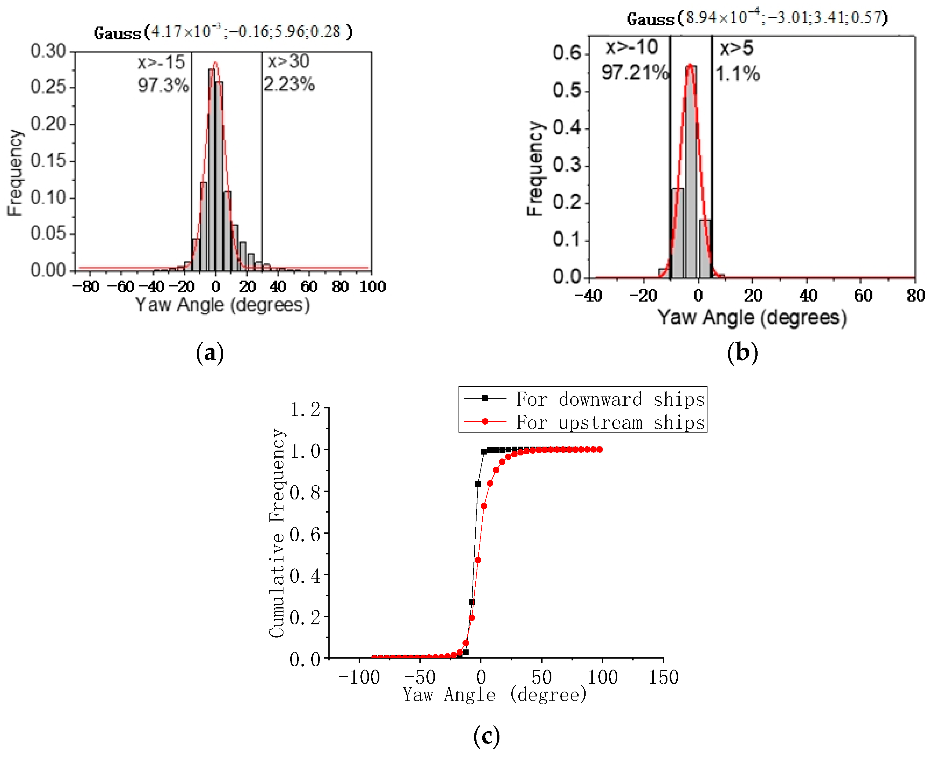
The yaw angle of the ship is defined as the intersection angle between the ship’s heading direction and the centerline of the channel. It directly relates to the angle of the ship that might strike the bridge pier. The statistical results of yaw angle are shown in Figure 10. The yaw angle of downstream ships is more concentrated than upstream ships. The yaw angles of 95% ships are between −10° and 5° for downstream ships and are between −20° and 20° for the upstream ships, hence the impact angle could be assumed as 20° in the oblique collision scenarios. The Gauss distribution is used to fit the distribution of yaw angle, and the regression equations are given as follows.
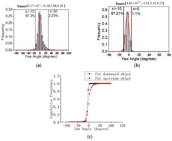
Figure 10.
Statistical results of ships yaw angle: (a) For upstream ships; (b) For downstream ships; (c) Cumulative frequency.
The coefficient of determination gives a statistical measurement that reflects the correlation between the design point and result assessed by the proposed formula. The coefficients of determination with 0.975 and 0.99 for passing ships in upstream and downstream are both close to one, which means that the Gauss distribution can fit the distribution of yaw angle very well. The statistical information including the weight, velocity, length and yaw angle of the passing ships would be used in the risk assessment of ship–bridge collision in Equation (16).
3. Risk Analysis of Ship–Bridge Collision
3.1. Risk Assessment Method
In the risk assessment of bridge against ship allision, the most important factor is the allision probability between ship and bridge. The most accurate way to calculate the collision probability is the long-term accident statistics method. But the ship–bridge allision accident is a small probability event, and the corresponding statistical data is generally not available during the design stage of bridge. The other method is using a mathematical model to calculate the allision probability between ships and bridges.
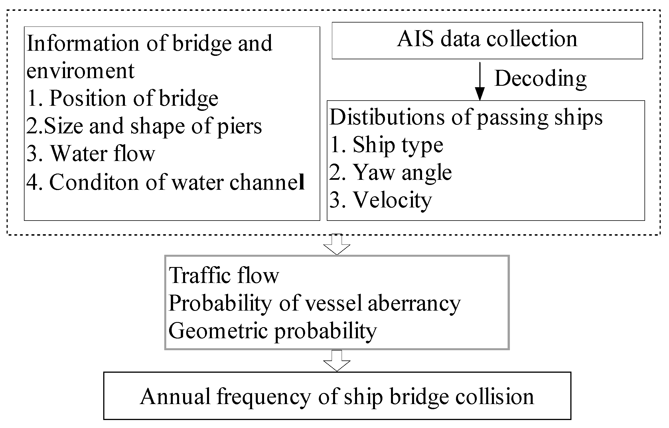
The AASHTO specification [11] provides a risk assessment method for ship–bridge allision, in which the probability of vessel aberrancy and geometric probability of sailing ships need to be determined first. The aberrancy probability refers to the abnormal navigation of the ship due to various reasons. Figure 11 shows the analysis flow chart of annual frequency of ship–bridge allision. The calculation method of the collision probability between ships and bridge in the AASHTO specification [11] is given as following expression.
where

Figure 11.
Analysis flow chart of annual frequency of ship–bridge collision.
AF: annual frequency of ship–bridge collision
N: annual number of ships classified by type, size, and load condition which could strike the bridge
PA: probability of vessel aberrancy
PG: geometric probability of a collision between an aberrant vessel and a bridge pier or span
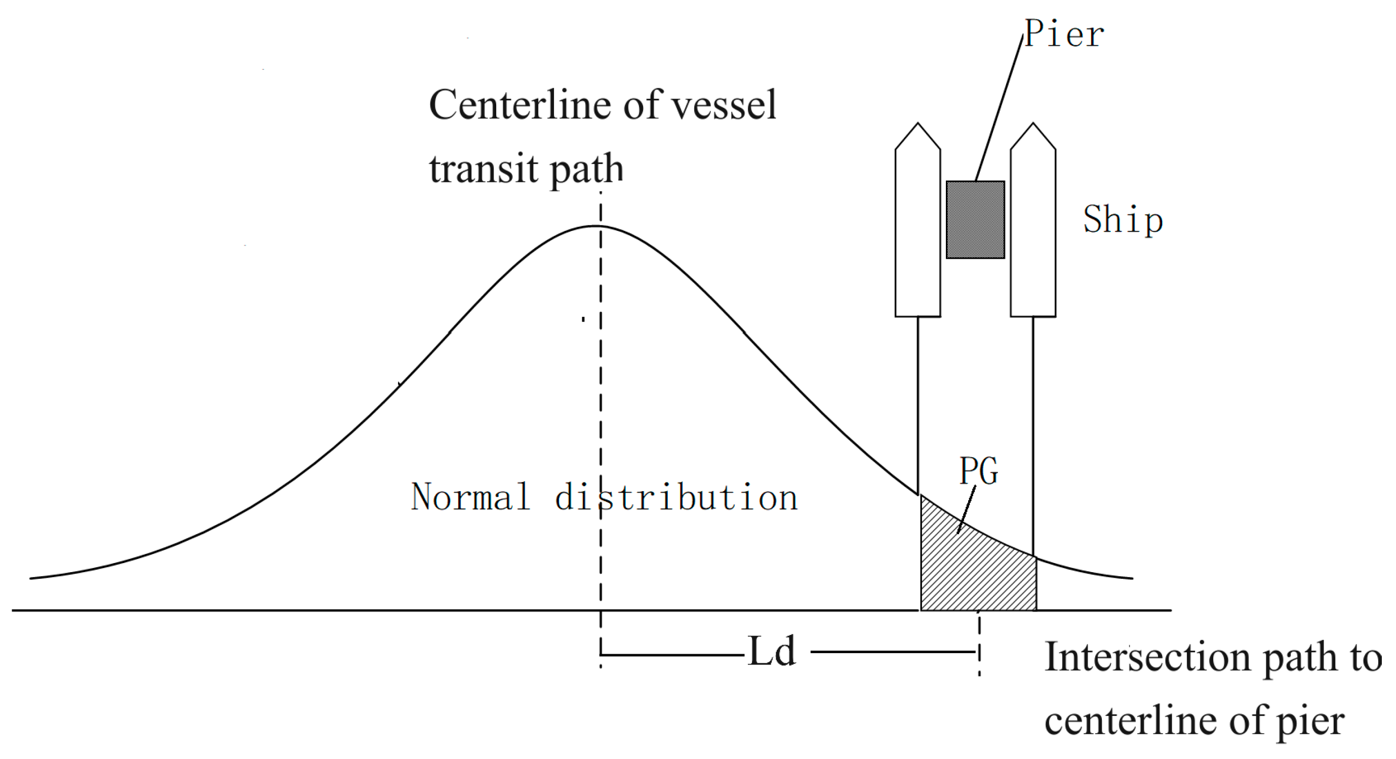
The geometric probability PG is determined by lateral distribution of ship traffic flow. The geometric probability PG is computed based on a normal distribution of vessel accidents about the centerline of the vessel transit path as shown in Figure 12. The lateral distribution () of ships in Figure 12 is defined as the distance between the centerline of vessel transit path and intersection path to centerline of pier. The standard deviation is assumed as length overall () of design ship for computing PG. The mean value and standard deviation of the ships from the statistical analysis of the AIS data are used to determine the distribution function, which is used to determine the lateral distribution (). The probability of vessel aberrancy PA is estimated by the following expression.
where
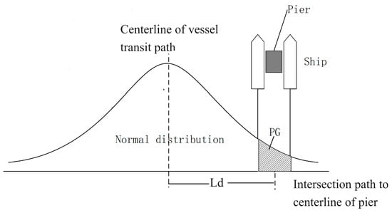
Figure 12.
Geometric probability (PG) of pier collision.
BR: the aberrancy base rate, which is 1.2 × 10⁻⁴ for barge and 0.6 × 10⁻⁴ for the other types of ship
RB: correction factor for bridge location;
RC: correction factor for current acting parallel to vessel transit path
RXC: correction factor for crosscurrents acting perpendicular to vessel transit path
RD: correction factor of vessel traffic flow density.
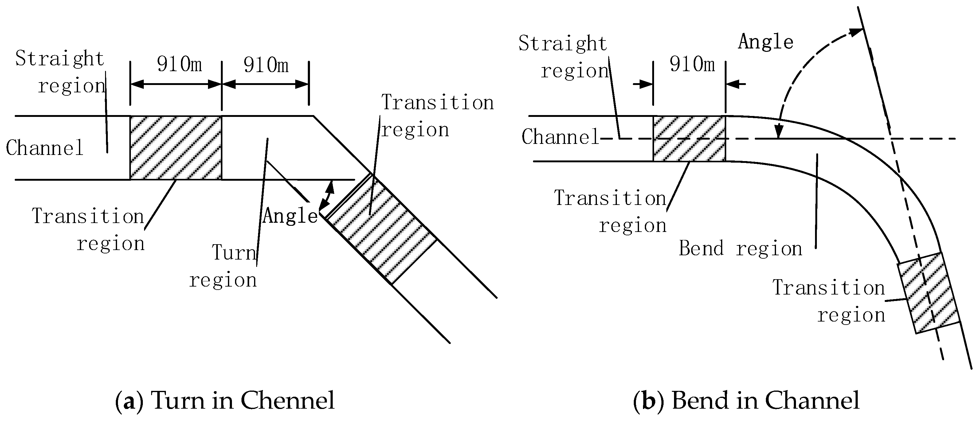
The bridge correction factor RB is related to the position of bridge in curving channel and the bending angle of channel, the relative relationship is shown in Figure 13. When the bridge is in the straight region, RB = 1.0, and for other areas, the bridge correction factor is calculated by the following expression.
where θ is the turn angle of channel and the measuring method of θ is shown in Figure 13. Equation (18) is used in transition region, and Equation (19) is used in turn region or bend region. For the parallel water flow correction factor RC and correction factor for crosscurrents acting perpendicular to vessel transit path RXC, the values are determined mainly by the speed and direction of water flow, which are calculated by
where VC (km/h) is the current velocity parallel to the vessel transit path; and VXC (km/h) is the current velocity perpendicular to the vessel transit path. The current velocity is obtained by statistical data, which is the mean velocity in one year in the AASHTO requirement.
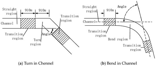
Figure 13.
Waterway region for bridge location.
The correction coefficient for ship traffic density RD is determined by the traffic density level. There are three density levels: low density, average density, and high density. The low density with RD = 1.0 means that the ships rarely meet, pass, or overtake each other in the vicinity of a bridge; the average density with RD = 1.3 means that the vessels occasionally meet, pass, or overtake each other in the vicinity of a bridge; the high density with RD = 1.6 indicates that the ships routinely meet, pass, or overtake each other in the vicinity of a bridge. The density levels will be determined by the statistical data of passing ships from AIS data.
3.2. Correction Method of Variables
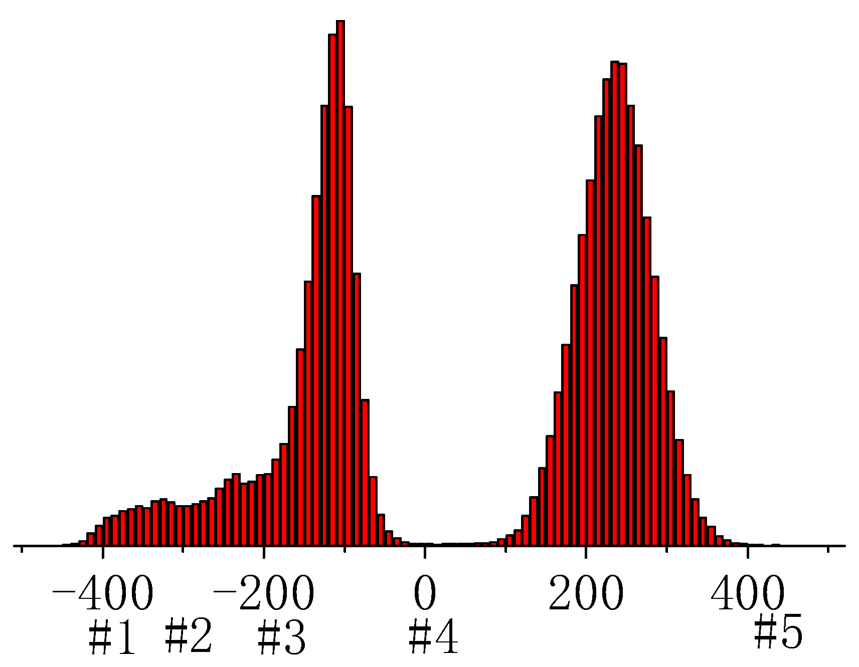
According to the statistical results from AIS data, the actual lateral distribution of passing ships is shown in Figure 14. The coordinate origin is set on the center of pier NO.4. In the AASHTO specification, the parameters of lateral distribution (Ld) are calculated by the centerline of channel and the mean length of ships passing the bridge in Figure 12. The mean value and standard deviation are very different between the AASHTO model and AIS data.

Figure 14.
Lateral distribution of passing ships.
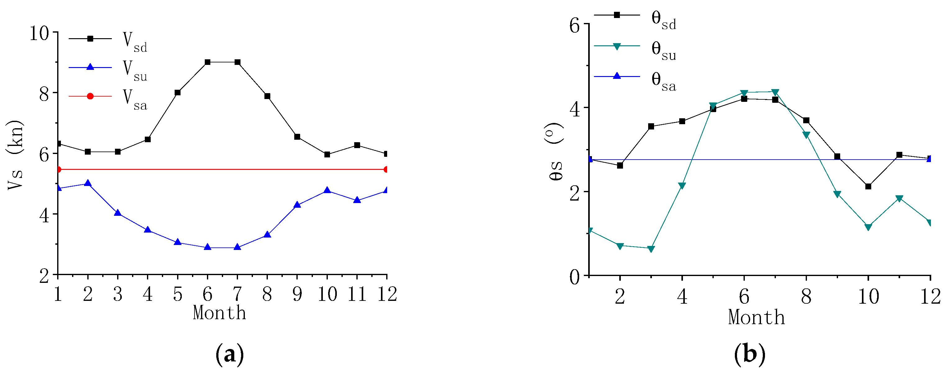
The mean value and standard deviation of the ships from the statistical analysis of the AIS data is different from recommendation values in AASHTO specification that developed from the historical data in the USA as shown in the Table 5, because the distributions of passing ships between them are different. The mean velocity and yaw angle from the statistical analysis of AIS data are plotted in Figure 15, in which θsd, θsu are the mean yaw angles of the passing ships for downstream and upstream in a month, and Vsd, Vsu are the mean velocities of the passing ship for downstream and upstream in a month. The angles θsu and Vsa are the average values of the yaw angle and velocities of the passing ship in three years. The AIS data has been collected over three years, including tide and current.
Table 5.
Statistical results of lateral distribution of passing ships.
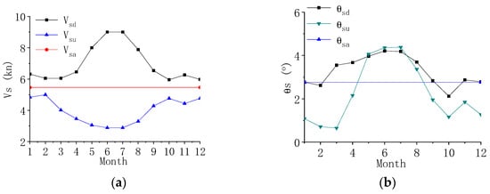
Figure 15.
Velocity and yaw angle of passing ships: (a) Velocity of passing ships; (b) Yaw angle of passing ships.
The velocity and yaw angle of upstream and downstream ships are very different during various months. The velocities of the ships between May and August are significantly larger than that of the other months for downstream. The mean value of ship velocity in every month has a significant discrepancy between upstream and downstream. Because the water flow significantly influences the velocity of ships passing under bridge, the water flow could push the downstream ship to move, and slow down the upstream ships. The maximum difference of the velocity of the ship passing in the upstream and downstream channels is about 6 kn, which occurs in June. The mean value of yaw angle in various months is also different because the direction of water flow changes in a year and then influences the direction of ship heading. The calculation of collision probability in the AASHTO specification mainly considers geometric probability and aberrancy probability. However, the corresponding parameters were developed by the historical data in the USA, which might be different from the circumstance of the new designed bridge in China.
The geometric probability PG is estimated by the lateral distribution of ships in bridge area. In the AASHTO requirement, the lateral distribution of ships in the vicinity of bridge is assumed to be a standard normal distribution. The mean value and standard deviation of ships from the statistical analysis from AIS data are very different from that recommended by the AASHTO specification as shown in Table 5. Moreover, the ship traffic flow varies with various water levels. Namely, the lateral distribution of ships’ track in bridge area is different in every month, as shown in Figure 4 and Figure 5.
The aberrancy probability PA in the AASHTO specification is estimated by the base probability of aberrancy and correction coefficient. For determining the water flow correction coefficient, the AASHTO model uses a constant water flow, in which the speed and direction are assumed as the same in one year. However, the water flow is different in a year. There are large differences in river flow in different periods, such as dry season, flood season, high tide, and low tide. The change of water flow’s speed is illustrated by the diverse of ships’ mean velocity in every month, as shown in Figure 15. The change of the flow’s direction is illustrated by the change of mean yaw angle every month. Hence, for obtaining more accurate results, it might not be suitable to calculate the correction coefficient of water flow by the mean value in a year.
The AIS data can provide more detailed statistical information of ships passing under bridges that could give more realistic value, which is used to calculate the lateral distribution and geometric probability. Considering the changes of water flow in a year, the aberrancy probability is calculated in every month, and the total aberrancy probability is calculated by
where I is the month, and PAi means the aberrancy probability in every month that is calculated in Equation (17). The correction coefficient of water flow is estimated by the mean value in a month.
There are several aspects that could affect the speed of ships, including the water flow and wind and so on. The water flow is the main factor that influences the velocity and heading directions of navigating ships. The velocity of water flow along the channel and cross velocity of water flow are estimated by the following expressions, respectively.
where I is the month; VCi is the along-velocity of water flow in the month; VXci is the cross-velocity of water flow in the month; and are the mean velocity of downstream ships and upstream ships in the month; and φi is the mean yaw angle in the month.
4. Collision Frequency
4.1. Geometric Probability
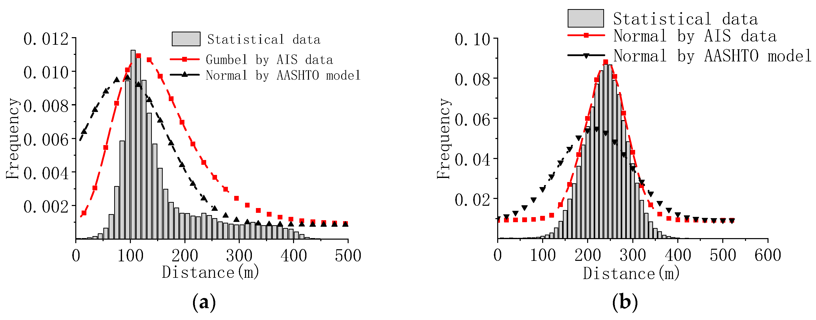
For comparison, the geometric probability and aberrancy probability are both assessed by the AIS data and AASHTO specification. The geometric probability is calculated by the lateral distribution () of the ships’ track in the bridge area in Figure 12 in the AASHTO specification. The lateral distribution of upstream and downstream ships based on AIS data is shown in Figure 16. The lateral distribution of the ships passing under bridge is approximately subject to normal distribution for the downstream, however, it follows Gumbel distribution more for upstream. In the AASHTO model, the mean value of normal distribution is equal to the centerline of channel, and the standard deviation is the mean length of ships. The parameters of ships’ lateral distribution are shown in Table 6. The coefficient of determination of various distributions are shown in Table 7.
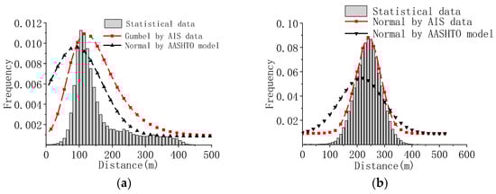
Figure 16.
Lateral distribution of passing ships: (a) In upstream channel between piers NO. 1 and NO. 4; (b) In downstream channel between piers NO. 4 and NO. 5.
Table 6.
The lateral distributions of ships.
Table 7.
Geometric probability PG (10−3).
The geometric probability calculated in AIS data and AASHTO model are shown in Table 7, which are very different. The geometric probability assessed by the AIS data are larger than that of AASHTO model for Piers NO. 1, NO. 2 and NO. 3, but smaller for Piers NO. 4 and NO. 5, because the geometric probability in AASHTO model is calculated according to the designed ship channel, but the actual traffic flows of ships are very different from the designed ship channel (see Figure 5). The mean value of their difference is about 19%. Hence, it is suggested to use AIS data to calculate geometric probability that should better reflect the actual situation.
4.2. Aberrancy Probability
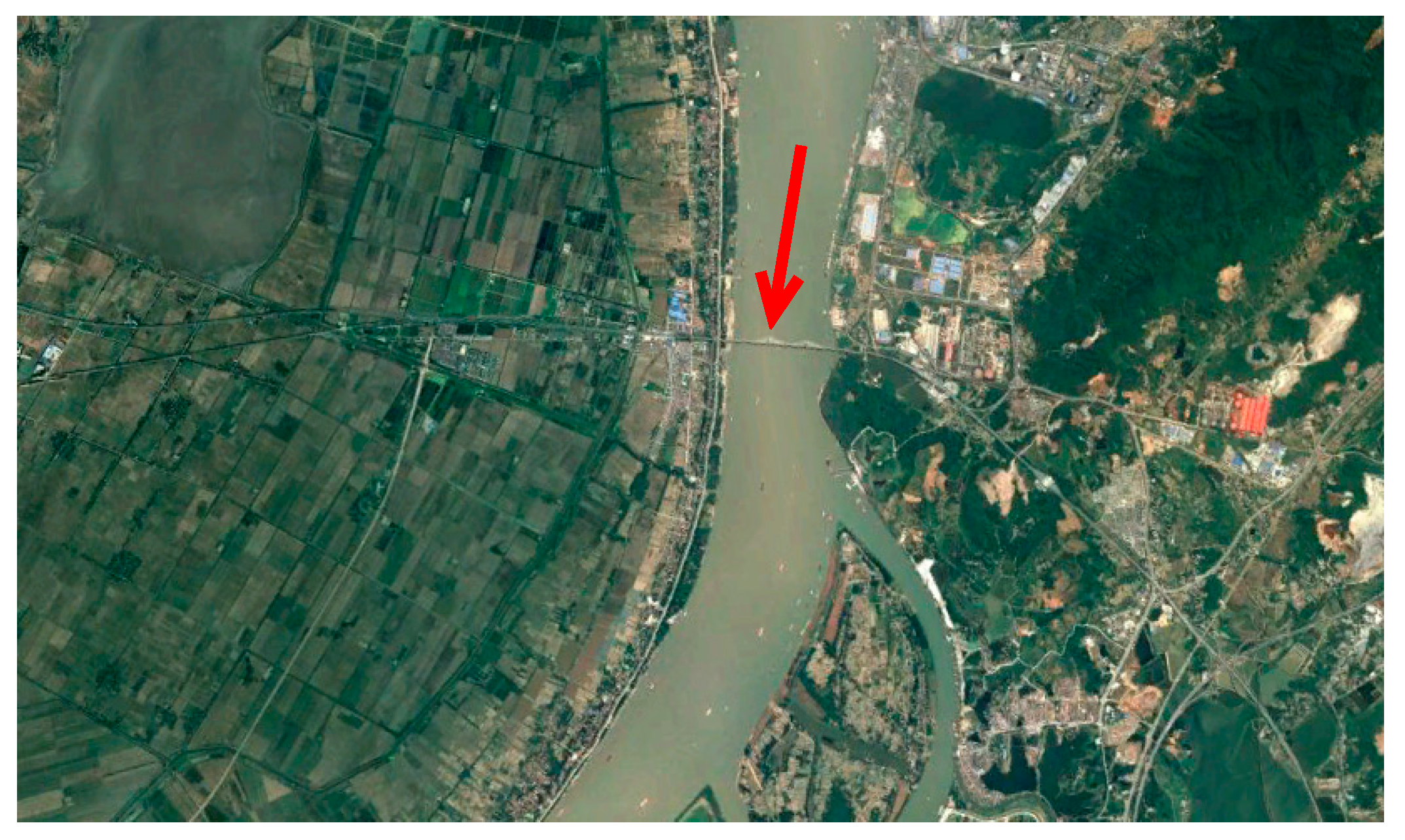
The calculation of the aberrancy probability PA needs to determine the corresponding correction coefficient according to the characteristics of different regions. From Table 1, the main type of ship passing under bridge is cargo ship. Therefore, the base probability of aberrancy BR is taken as 1.2 × 10⁻⁴ in the AASHTO model. According to the Table 1, the daily number of ships passing under the bridge is around 1000. Hence, the density level of ship traffic in this bridge area is high density, and the correction coefficient for ship traffic density RD is equal to 1.6. For the correction coefficient of bridges’ position RB as shown in Figure 17, the bridge is located in a transition region, and the angle between the river and bridge is about 58°. Hence, according to the Equation (3), RB is set as 1.64. The mean speed of water flow in a year is about 1.49 kn, and the mean angles of water flow for upstream channel and downstream channel are about 3.27° and 2.25°.

Figure 17.
Geographic location of the bridge (The red arrow indicates the location of the bridge).
After determining the relevant correction factors, the aberrancy probability PG is calculated, and the results are shown in Table 8, in which Type I means that PA is calculated in Equation (17) in AASHTO model, and Type II means that the PA is assessed in Equation (22) with considering the variation of velocity and direction water flow in every month. The difference of the aberrancy probability with and without considering the changes of water flow velocity is relatively small, because the velocity of the water flow is small, and the change of the status in every month is also slight. The probability of vessel aberrancy with large velocity of downstream ship is larger than that of upstream ship. Hence, strengthening legal regulations and limitation of ship speed in the bridge area is a possible application solution to reduce the impact accident. The average velocity and direction of water flow could be adopted in the collision risk assessment for simplifying the calculation procedure.
Table 8.
Probability of vessel aberrancy (PA).
4.3. Collision Frequency of Bridge and Ships
After calculating the geometric probabilities and aberrancy probabilities as shown in Table 3 and Table 4, the ship–bridge collision frequency is assessed by Equation (1). The results of collision frequency with various correction methods are shown in Table 9. R0 R1, R2 and R3 are the annual collision frequency assessed by risk model in the AASHTO requirement [10] without correction or with considering different correction methods, which is explained as following.
Table 9.
Collision frequencies with various methods.
- R0: using the parameters recommended by AASHTO requirement without considering correction.
- R1: with considering the change of flow velocity and direction in various months.
- R2: the geometric probability is corrected by using AIS data.
- R3: with considering the change of flow velocity and direction in various months, and using AIS data to calculate the geometric probability, respectively.
Table 9 shows the collision frequencies with various correction methods. The collision frequency R0 without considering correction and R1 with considering the change of flow velocity and direction in various months are 8.15 and 8.43. Their difference is only 3.4%, which means that the influence of velocity and direction of water flow on collision frequency is slight for the present circumstance under consideration. The reason might be the variation of velocity and direction of water flow is small in various months.
The results of R2 and R3 are also close. Their difference is also whether considering the influence of water flow. This means that the influence of velocity and direction of water flow on the collision frequency is slight as well. The annual collision frequency (R2) using the geometric probability corrected by using AIS data is 6.638, which is 18.5% larger than R1 without correction, because the geometric probability mainly depends on the lateral distributions of passing ships. From Figure 16, the actual lateral distributions of passing ships obtained from AIS data is very different from that of the AASHTO model. The distribution of ships passing under bridge in the AASHTO specification is assumed as Normal distribution, which is more like Gumbel distribution. The total geometric probability calculated in AIS data and AASHTO model are 119 and 97 in Table 7, and their corresponding difference is 22.7%.
Although the total collision frequency between R2 and R0 are significantly different, the annual collision frequency R2 of NO. 4 and NO. 5 are 0.27 and 0.003, which is significantly smaller than R0 with 4.52 and 0.23. The centerline of vessel transit path is assumed as at the center of the designed channel in the AASHTO specification, but is very different from the actual circumstance (see Figure 14). This indicates that the distribution of ships passing under the bridge might be very different from the assumption in the AASHTO specification that was derived from historical data in the USA, which significantly influenced the annual total collisions frequency. The collision frequency R2 of NO. 1 and NO. 2 is significantly higher than R0, because some upstream ships did not follow the traffic rules and navigated in a restricted navigation zone, which increased the collision probability of bridge piers in this area.
Hence, it is suggested to use actual information of passing ships from AIS data in the collision frequency analysis, especially when the actual centerline of vessel transit path is different from the designed center of a navigable vessel channel. It must be noted that the estimated risk in the design stage of bridge cannot be fully equated with actual risk because probability and consequence estimate that make up a risk estimate may change after a bridge is built. This conclusion is derived from the relative comparison in the AASHTO specification using the recommendation values from the historical data in the USA and the statistical information of passing ships from AIS data. Because although the actual information of passing ships from AIS data could provide the results that could predict the actual circumstance, the verification of assessment results is still difficult to conduct at the present stage since the impact accident has not actually occurred yet, which might be studied when the accident occurs in the future.
5. Conclusions
The influential parameters of ships passing under bridge from AIS data are investigated and compared with the value recommended by the AASHTO specification. The risk analysis of ship–bridge collision with various methods are conducted. The main conclusions are derived as following.
- The influence of velocity and direction of water flow on collision frequency is slight, which could adopt an average value in the collision risk assessment for simplifying the calculation procedure.
- The velocity for upstream and downstream ships are very different, which significantly influence the risk assessment result and should be considered separately in the risk analysis of bridge anti-collision.
- Since the water depth of river could change in different seasons that would change the navigation path of ships, the actual lateral distributions of ships passing under bridge are generally different from the designed vessel transit path, which significantly affects the geometric probability.
- The total annual collision frequency considering the actual lateral distribution from AIS data is around 22% smaller than that without correction in the AASHTO specification. This difference is more significant for various piers. It is suggested to use actual information of passing ships from AIS data in the collision frequency analysis, and then the corresponding assessment risk results could more reflect the actual circumstance.
Author Contributions
J.P.: Investigation, Validation, Editing, Supervision. Y.W.: Computation, Writing—Original draft preparation. T.W.: Data analysis. M.X.: Conceptualization, Methodology and Reviewing. All authors have read and agreed to the published version of the manuscript.
Funding
This work has been supported by the National Natural Science Foundation of China (Grant No. 52371319, 12372358).
Institutional Review Board Statement
Not applicable.
Informed Consent Statement
Not applicable.
Data Availability Statement
The authors declare that the data presented in this study are available upon request.
Conflicts of Interest
No conflict of interest exits in the submission of this manuscript, and manuscript is approved by all authors for publication. I would like to declare on behalf of my co-authors that the work described was original research that has not been published previously, and not under consideration for publication elsewhere, in whole or in part. All the authors listed have approved the manuscript that is enclosed.
References
- Manen, S.E.A. Ship Collision Due to the Presence of Bridges; Technical Report; PIANC General Secretariat: Brussels, Belgium, 2001. [Google Scholar]
- Larsen, O.D. Ship Collision with Bridges: The Interaction between Vessel Traffic and Bridge Structures; IABSE Structural Engineering Document 4; IASBE-AIPC-IVBH: Zurich, Switzerland, 1993. [Google Scholar]
- Pan, J.; Wang, T.; Huang, S.W.; Xu, M.C. Investigation of assessment method of axial crushing force of rake bow for bridge against ship collision. Ocean Eng. 2023, 269, 113498. [Google Scholar] [CrossRef]
- Gholipour, G.; Zhang, C.W.; Mousavi, A.A. Nonlinear numerical analysis and progressive damage assessment of a cable-stayed bridge pier subjected to ship collision. Mar. Struct. 2020, 69, 102662. [Google Scholar] [CrossRef]
- Pedersen, P.T.; Chen, J.; Zhu, L. Design of bridges against ship collisions. Mar. Struct. 2020, 74, 102810. [Google Scholar] [CrossRef]
- Kunz, C.U. Ship bridge collision in river traffic, analysis and design practice. Ship Collis. Anal. 1998, 13–21. [Google Scholar]
- Pedersen, P.T.; Valsgaard, S.; Olsen, D.; Spangenberg, S. Ship impacts: Bow collisions. Int. J. Impact Eng. 1993, 13, 163–187. [Google Scholar] [CrossRef]
- Pedersen, P.T.; Zhang, S. The mechanics of ship impacts against bridge. In Proceedings of the International Symposium on Advances in Ship Collision Analysis, Copenhagen, Denmark, 1 January 1998; pp. 41–51. [Google Scholar]
- Lee, S.L. Ship collision risk assessment and sensitivity analysis for sea-crossing bridges. J. Korean Soc. Civ. Eng. 2013, 33, 1753–1763. [Google Scholar]
- Son, W.J.; Cho, I.S. Development of collision risk assessment model for bridge across waterways based on traffic probability distribution. Ocean Eng. 2022, 266, 112844. [Google Scholar] [CrossRef]
- AASHTO. Guide Specifications and Commentary for Vessel Collision Design of Highway Bridges; American Association of State Highway and Transportation Official: Washington, DC, USA, 2007. [Google Scholar]
- IMO. SOLAS Consolidated; IMO 4 Albert Embankment: London, UK, 2009. [Google Scholar]
- Mou, J.; Tak, C.; Ligteringen, H. Study on collision avoidance in busy waterways by using AIS data. Ocean Eng. 2010, 37, 483–490. [Google Scholar] [CrossRef]
- Hansen, M.G.; Randrup-Thomsen, S.; Askeland, T.; Ask, M. Bridge crossing at Sognefjorden-ship collision risk studies. In Collision and Grounding of Ship and Offshore Structures; CRC Press/Taylor and Francis Group: London, UK, 2013; pp. 9–17. [Google Scholar]
- Zaman, M.B.; Kobayashi, E.; Wakabayashi, N. Fuzzy FMEA model for risk evaluation of ship collisions in the Malacca Strait: Based on AIS data. J. Simul. 2014, 8, 91–104. [Google Scholar] [CrossRef]
- Wu, B.; Yip, T.L.; Yan, X.P.; Guedes Soares, C. Fuzzy logic based approach for ship-bridge collision alert system. Ocean Eng. 2019, 187, 106152. [Google Scholar] [CrossRef]
- Xiao, F.L.; Ligteringen, H.; Gulijk, C.; Ale, B. Comparison study on AIS data of ship traffic behavior. Ocean Eng. 2015, 95, 84–93. [Google Scholar] [CrossRef]
- Wu, X.; Rahman, A.; Zaloom, V.A. Study of travel behavior of vessels in narrow waterways using AIS data—A case study in Sabine-Neches Waterways. Ocean Eng. 2018, 147, 399–413. [Google Scholar] [CrossRef]
- Fiorini, M.; Capata, A.; Bloisi, D.D. AIS data visualization for maritime spatial planning (MSP). Int. J. e-Navig. Marit. Econ. 2016, 5, 45–60. [Google Scholar] [CrossRef]
- Horteborn, A.; Ringsberg, J.W. A method for risk analysis of ship collisions with stationary infrastructure using AIS data and a ship manoeuvring simulator. Ocean Eng. 2021, 235, 109396. [Google Scholar] [CrossRef]
- Cai, M.Y.; Zhang, J.F.; Zhang, D.; Yuan, X.L.; Guedes Soares, C. Collision risk analysis on ferry ships in Jiangsu Section of the Yangtze River based on AIS data. Reliab. Eng. Syst. Saf. 2021, 215, 107901. [Google Scholar] [CrossRef]
- Cauteruccio, F.; Terracina, G.; Ursino, D. Generalizing identity-based string comparison metrics: Framework and techniques. Knowl.-Based Syst. 2020, 187, 104820. [Google Scholar] [CrossRef]


Disclaimer/Publisher’s Note: The statements, opinions and data contained in all publications are solely those of the individual author(s) and contributor(s) and not of MDPI and/or the editor(s). MDPI and/or the editor(s) disclaim responsibility for any injury to people or property resulting from any ideas, methods, instructions or products referred to in the content. |
© 2024 by the authors. Licensee MDPI, Basel, Switzerland. This article is an open access article distributed under the terms and conditions of the Creative Commons Attribution (CC BY) license (https://creativecommons.org/licenses/by/4.0/).