Application of Regularized Meshless Method with Error Estimation Technique for Water–Wave Scattering by Multiple Cylinders

Abstract

In this manuscript, we will apply the regularized meshless method, coupled with an error estimation technique, to tackle the challenge of modeling oblique incident waves interacting with multiple cylinders. Given the impracticality of obtaining an exact solution in many real engineering problems, we introduce an error estimation technique designed to achieve reliable solutions. This technique excels in providing dependable solutions that closely approximate analytical solutions. An additional advantage is its capacity to identify the optimal number of points for both source and collocating points, thereby enhancing computational efficiency. The validity of the proposed method will be demonstrated through three numerical cases, presenting results that exhibit substantial agreement.

1. Introduction

The interaction between waves and structures is a significant concern, particularly when considering potential flow around essential shapes such as circular cylinders, elliptic cylinders, and thin airfoils. Traditionally, textbooks have utilized the complex variables method to derive exact solutions for these fundamental problems. Chen et al. [1] introduced a series solution and addressed numerical instability in the potential flow problem around circular, elliptical cylinders, and thin airfoils. This was achieved through the utilization of the boundary integral equation along with a degenerate kernel. The primary breakthrough highlighted in [1] was the effective utilization of the boundary integral equation to address, for the first time, the potential flow problem around a cylinder. Expanding upon successful experiences, the potential flow problem was extended from a single circular cylinder to double circular cylinders through the application of the degenerate kernel of bipolar coordinates [2]. With the aid of the degenerate kernel of bipolar coordinates, deriving the exact solution in series form for the potential flow problem around double circular cylinders becomes feasible. Hung et al. [3] designed a three-dimensional wave flume to simulate nonlinear wave behavior, utilizing the meshless generalized finite difference method (GFDM) in combination with the second-order Runge–Kutta method (RKM). The model’s accuracy was validated through various numerical benchmarks, covering scenarios of transient extreme waves, irregular waves, and focused waves. The numerical results demonstrated strong agreement with physical phenomena, emphasizing the effectiveness of employing meshless GFDM in conjunction with the second-order RKM. The nonlinear regularized long-wave (RLW) equation, a fundamental equation in shallow-water waves, proves proficient in describing a variety of significant physical phenomena. The RLW equation can be solved using the Caputo fractional derivative in combination with the Homotopy Perturbation Yang Transform Method (HPTM) and Yang transform decomposition method (YTDM), as outlined in the methodology proposed by [4]. We derived a series solution for the model by employing the method of fundamental solutions (MFS) [5]. A traditional limitation of MFS was the challenge in determining the distance between the collocation point and the source point. Engineers faced difficulties in assessing the correctness of results, as different distances would lead to varied solutions. The study conducted by [5] focused on the interaction of waves with multiple circular cylinders, employing the MFS along with an error estimation technique. This technique proved instrumental in overcoming the traditional drawback associated with MFS. Simultaneously, the error estimation technique offers the ability to determine the optimal number of collocation points.

The technique of error estimation is frequently employed to evaluate the variability within linear regression models. In his research, Singh [6] investigated the estimation of error variance in linear regression models, wherein the variances display characteristics resembling a multivariate Student-t distribution with unknown degrees of freedom. Liu et al. [7] introduced an innovative estimator for error variance that is applicable to both low- and high-dimensional models. In their work, Wang et al. [8] presented the natural adaptive lasso as a method to address multiple variances within high-dimensional models. Guo and Jacob [9] presented a natural lasso estimator for error variance and an associated estimator to manage the coefficient vector in high-dimensional linear models. A significant advantage of their approach lies in its ability to derive theoretical results without relying on assumptions about the design matrix or true regression coefficients. This method’s utility extends to the estimation of error variance in genomic selection. Genomic selection necessitates managing large datasets, presenting a well-acknowledged challenge. As the number of markers is typically greater than the sample size in genomic selection, the conventional ordinary least squares estimation technique may be insufficient for accurate modeling. Guha Majumdar et al. [10] proposed the Bootstrap-RCV and Ensemble method to handle ultrahigh-dimensional data. In the realm of statistical research, where error estimation has seen limited exploration, our work stands as a pioneering endeavor in effectively integrating error estimation techniques with numerical methods. The key advantage of our proposed error estimation technique is its adaptability to any numerical method, enhancing the computational precision of the chosen approach.

Numerous scholars and mathematicians have contributed to the development of various numerical methods, including the finite difference method, finite element method, boundary element method, and meshless method. These numerical techniques facilitate engineers in effortlessly deriving solutions to problems. Derived from the boundary element method, several meshless methods have emerged, with a key distinction being that the meshless method relies solely on points, eliminating the need for elements. The boundary knot method (BKM) [11,12,13,14], boundary particle method [15], Trefftz method [16], and MFS [17,18,19] belong to one kind of boundary-discretization-type meshless methods.

Since its introduction by Kupradze and Aleksidze in 1964 [17], the MFS has garnered significant attention in the field of model creation. Its advantages include avoiding the need for cumbersome boundary discretization, eliminating singular or hypersingular integrals on the boundary, evaluating the solution in the interesting domain without extra quadrature, and requiring minimal input data preparation. Essentially, the MFS stands out as an appealing solution for addressing complex geometry problems due to its meshfree nature, rapid convergence, and adaptability to high-dimensional challenges. It is capable of handling complex boundary conditions (B.C.s) and can accommodate abrupt changes in the domain’s geometry [20]. By fine-tuning the location distance, the MFS can achieve a highly efficient algorithm that surpasses the accuracy achievable with traditional methods. This characteristic serves as both an advantage and a disadvantage. The challenge lies in the fact that the optimal distance is unknown, necessitating users to engage in continual testing. Determining the optimal location distance in advance can transform the conventional MFS into a highly appealing and dominant numerical method. However, a major drawback of the MFS is the requirement to establish the distance between the source point and the collocation point. In our experience, varying distances can result in different solutions in the field, posing a challenge in confirming the accuracy of a field solution when an exact one is unavailable. In addressing the limitations of MFS, Chen et al. [21] introduced a novel meshless method, now called the Regularization Meshless Method (RMM). This method can distribute observation and source points simultaneously along the physical boundary without the need to consider the offset distance between source and observation points. A crucial aspect involves the introduction of the subtracting and adding-back technique [21,22,23], which effectively regularizes the singularity and hypersingularity of the kernel functions. The diagonal terms of the influence matrices can be extracted when the offset distance between source and observation points is zero, using the subtracting and adding-back technique. The RMM has proven successful in addressing a range of problems in many areas [24]. Conversely, numerous real engineering problems frequently lack exact solutions, prompting engineers to depend on numerical solutions for decision-making. To meet the demands of engineers, the numerical method may be required to provide a high-precision numerical solution. We have devised an error estimation technique to assist numerical methods in achieving high-precision numerical results. Employing this error estimation technique provides four distinct advantages. Firstly, it provides a dependable solution for approximating the analytical solution. Secondly, it aids in determining the optimal number of points for both source and collocation points. Thirdly, the error estimation technique enables the development of a scheme refinement for the adaptive distribution of source points. Lastly, it can be seamlessly integrated with various numerical methods. We effectively utilized the MFS in tandem with an error estimation technique to tackle the challenge of water waves passing through multiple cylinders [5]. The primary drawback of MFS is the undetermined distance between the source point and the collocation point. However, by integrating MFS with an error estimation technique, conventional limitations can be overcome while retaining its inherent advantages. This approach simultaneously offers insights into the optimal number of collocation points.

This paper represents our initial exploration of employing RMM in tandem with an error estimation technique. Our goal is to tackle the challenges presented by waves passing through two or four circular cylinders by utilizing the RMM in conjunction with an error estimation technique. The inclusion of the error estimation technique enables the determination of the optimal number of collocation points for the RMM. The results obtained through the proposed method will be compared with those presented in [25]. The paper is organized as follows: Section 2 begins with the problem statement for the water wave problem with multiple cylinders. The derivation of RMM and the error estimation technique will be introduced in the Section 3. Section 4 illustrates the accuracy of the current method through numerical results. In conclusion, Section 5 delves into related works.

2. Problem Statement

Water Wave Problem

In this paper, we consider an irrotational, inviscid, and incompressible fluid, utilizing the linearized water–wave theory to investigate small-amplitude waves. The velocity potential $\Psi (\tilde{x},z,t)$ satisfies the Laplace equation, expressed as:

$${\nabla }^2\Psi (\tilde{x},z,t)={\nabla }^2\Psi (x,y,z,t)=0,\tilde{x}\in D.$$

(1)

Considering the presence of m vertical cylinders mounted at $z=-h$ and extending upward to the free surface, the seabed boundary condition is as follows:

$${\left(\frac{\partial \Psi }{\partial z}\right)}_{z=-h}=0,z=-h,$$

(2)

and the linearized condition on the free surface is:

$${\left(\frac{-{\omega }^2}{g}\Psi +\frac{\partial \Psi }{\partial z}\right)}_{z=0}=0,$$

(3)

where g, ω, and h represent gravitational acceleration, angular frequency, and water depth, respectively. The boundary condition on the cylinder surface is fulfilled as:

$$\frac{\partial \Psi }{\partial n_{\tilde{x}}}=0,-h\le z\le 0.$$

(4)

By employing the technique of separating variables for both the spatial and time domains, we have:

$$\Psi (\tilde{x},z,t)=\mathrm{Re}\left\{u_W(\tilde{x})f(z)e^{-i\omega t}\right\},$$

(5)

where:

$$f(z)=\frac{-igA}{\omega }\frac{\cosh k(z+h)}{\cosh kh},$$

(6)

in which $A$ and $k$ are the amplitude of incident wave and wave number, respectively. Substituting Equations (5) and (6) into Equation (1), $u_W(\tilde{x})$ satisfies the Helmholtz equation [5,26], as follows:

$$\left({\nabla }^2+k^2\right)u_W(\tilde{x})=0,\tilde{x}\in D.$$

(7)

The dispersion relationship is:

$$k\tanh kh=\frac{{\omega }^2}{g}.$$

(8)

By employing the superposition method, $u_W(\tilde{x})$ can be decomposed into the incident field of wave $u_{inc}(\tilde{x})$ and the unknown scattering field $u_{sca}(\tilde{x})$ as:

$$u_W(\tilde{x})=u_{inc}(\tilde{x})+u_{sca}(\tilde{x}),\tilde{x}\in D,$$

(9)

in which ${\theta }_{inc}$ is the angle of incident wave. The incident wave adopts $u_{inc}(\tilde{x})=e^{ikr\cos (\theta -{\theta }_{inc})}$. Considering m cylinders, Equation (4) can be reformulated as:

$$t_{sca}(\tilde{x})=\frac{\partial u_{sca}(\tilde{x})}{\partial n_{\tilde{x}}}=0,\tilde{x}\in B_i,i=1,2,\dots m.$$

(10)

The free surface boundary condition is fulfilled as:

$${\left(\frac{-{\omega }^2}{g}{u}_{sca}(\tilde{x})+\frac{\partial u_{sca}(\tilde{x})}{\partial z}\right)}_{z=0}=0.$$

(11)

The two components of the first-order force, F_j, on the j-th cylinder surface are determined by integrating the pressure over the circular boundary, as illustrated below:

$$F_j=-\frac{\rho gAr}{k}\tanh kh{\displaystyle {\int }_0^{2\pi }{u}_W(\tilde{x})\left\{\begin{array}{c}\cos {\theta }_j\\ \sin {\theta }_j\end{array}\right\}d\theta },$$

(12)

where $r$ is the radius of the j-th cylinder.

3. Numerical Method

3.1. Meshless Formulation Using Radial Basis Functions (RBFs)

By employing the RBF technique of the dual formulation [27,28], the representation of the solution can be expressed as follows:

$$\begin{gathered} u({\tilde{x}}_i)={\displaystyle \sum _{j=1}^{N}T({\tilde{x}}_i,{\tilde{s}}_j){\beta }_j}, \\ =\left\{\begin{array}{c}{\displaystyle \sum _{j=1}^{N_0}T({\tilde{x}}_i,{\tilde{s}}_j){\beta }_j}+{\displaystyle \sum _{j=N_0+1}^{N_0+N_1}T({\tilde{x}}_i,{\tilde{s}}_j){\beta }_j}+\dots +{\displaystyle \sum _{j=N_0+\dots +N_{m-1}+1}^{N}T({\tilde{x}}_i,{\tilde{s}}_j){\beta }_j},\tilde{x}\in D (\mathrm{interior} \mathrm{type})\\ {\displaystyle \sum _{j=1}^{N_1}T({\tilde{x}}_i,{\tilde{s}}_j){\beta }_j}+{\displaystyle \sum _{j=N_1+1}^{N_1+N_2}T({\tilde{x}}_i,{\tilde{s}}_j){\beta }_j}+\dots +{\displaystyle \sum _{j=N_1+\dots +N_{m-1}+1}^{N}T({\tilde{x}}_i,{\tilde{s}}_j){\beta }_j},\tilde{x}\in D (\mathrm{exterior} \mathrm{type})\end{array}\right. \end{gathered}$$

(13)

$$\begin{gathered} t({\tilde{x}}_i)={\displaystyle \sum _{j=1}^{N}M({\tilde{x}}_i,{\tilde{s}}_j){\beta }_j}, \\ =\left\{\begin{array}{c}{\displaystyle \sum _{j=1}^{N_0}M({\tilde{x}}_i,{\tilde{s}}_j){\beta }_j}+{\displaystyle \sum _{j=N_0+1}^{N_0+N_1}M({\tilde{x}}_i,{\tilde{s}}_j){\beta }_j}+\dots +{\displaystyle \sum _{j=N_0+\dots +N_{m-1}+1}^{N}M({\tilde{x}}_i,{\tilde{s}}_j){\beta }_j},\tilde{x}\in D (\mathrm{interior} \mathrm{type})\\ {\displaystyle \sum _{j=1}^{N_1}M({\tilde{x}}_i,{\tilde{s}}_j){\beta }_j}+{\displaystyle \sum _{j=N_1+1}^{N_1+N_2}M({\tilde{x}}_i,{\tilde{s}}_j){\beta }_j}+\dots +{\displaystyle \sum _{j=N_1+\dots +N_{m-1}+1}^{N}M({\tilde{x}}_i,{\tilde{s}}_j){\beta }_j},\tilde{x}\in D (\mathrm{exterior} \mathrm{type})\end{array}\right. \end{gathered}$$

(14)

where ${\tilde{x}}_i$ and ${\tilde{s}}_j$ represent the i-th collocation point and j-th source point, respectively. ${\beta }_j$ are the generalized unknown coefficients obtained using the single and double-layer potential approaches, respectively. $N$ and $N_0$ are the total number of source points and the number of source points on the outer boundary, respectively. The kernel functions are provided below:

$$T({\tilde{x}}_i,{\stackrel{⌢}{s}}_j)=\frac{\partial U({\tilde{x}}_i,{\tilde{s}}_j)}{\partial n_{\tilde{s}}}=-\frac{i\pi k}{2}{H}_1^1(k{r}_{ij})\frac{n_k{y}_k}{r_{ij}}$$

(15)

$$M({\tilde{x}}_i,{\tilde{s}}_j)=\frac{{\partial }^{2}U({\tilde{x}}_i,{\tilde{s}}_j)}{\partial n_{\tilde{s}}\partial n_{\tilde{x}}}=\frac{i\pi k}{2}[k{H}_2^1(k{r}_{ij})\frac{y_k{y}_l{n}_k{n}_l}{r_{ij}^2}-H_1^1(k{r}_{ij})\frac{n_k{n}_l}{r_{ij}}]$$

(16)

where $H_1^{(1)}(k{r}_{ij})$ and $H_1^{(2)}(k{r}_{ij})$ are the Hankel functions of the first kind of the first and second order, respectively. $r_{ij}$ is the distance between ${\tilde{x}}_i$ and ${\tilde{s}}_j$, $y_k=({\tilde{s}}_j-{\tilde{x}}_i)$, $i=\sqrt{-1}$. $n_k$ is the kth component of the outward normal vector at source point ${\tilde{s}}_j$, and ${\overline{n}}_k$ is the kth component of the outward normal vector at field point ${\tilde{x}}_i$. It is noted that the double layer potentials in Equations (13) and (14) have both singularity and hypersingularity when ${\tilde{s}}_j$ approaches ${\tilde{x}}_i$. For this reason, the MFS requires a controversial auxiliary boundary. Although selecting an auxiliary boundary helps prevent singularity in the kernel function, introducing an offset distance between the auxiliary boundary (B′) and the actual boundary (B) poses new challenges. The offset distance cannot be arbitrarily determined. To address this limitation, ${\tilde{s}}_j$ is distributed along the actual boundary using the regularization techniques proposed below. The reason for opting for the double-layer potential, in contrast to the single-layer potential utilized in the proposed method for the RBFs, is to exploit the regularization offered by the subtracting and adding-back technique. This obviates the requirement for an offset distance when assessing the diagonal coefficients of influence matrices, as elaborated. If single-layer potential is employed, the regularization technique of subtracting and adding back will be unsuccessful [29]. Hence, the single-layer potentials cannot be selected as RBFs.

3.2. Derivation of Diagonal Coefficients of Influence Matrices for an Arbitrary Domain Using the Regularization Meshless Method (RMM)

As the collocation point ${\tilde{x}}_i$ approaches the source point ${\tilde{s}}_j$, the potentials in Equaions (13) and (14) become singular. For the interior and exterior problems with multiple holes, Equations (13) and (14) require regularization through the subtracting and adding-back technique [21], as follows:

3.2.1. Interior Problem

For the interior problem, the regularization of Equation (13) is shown below:

$$\begin{array}{ll}u({\tilde{x}}_i^O)& ={\displaystyle \sum _{j=1}^{i-1}T({\tilde{x}}_i^O,{\tilde{s}}_j^O){\beta }_j}+\dots +{\displaystyle \sum _{j=i+1}^{N_0}T({\tilde{x}}_i^O,{\tilde{s}}_j^O){\beta }_j}+{\displaystyle \sum _{j=N_0+1}^{N_0+N_1}T({\tilde{x}}_i^O,{\tilde{s}}_j^I){\beta }_j}+\dots \\ & +{\displaystyle \sum _{j=N_0+\dots N_{m-1}+1}^{N}T({\tilde{x}}_i^O,{\tilde{s}}_j^I){\beta }_j}-\left[{\displaystyle \sum _{j=1}^{N_0}\overline{T}({\tilde{x}}_i^I,{\tilde{s}}_j^I){\beta }_j-T({\tilde{x}}_i^O,{\tilde{s}}_i^O){\beta }_i}\right], {\tilde{x}}_i^O\in B_p, p=0\end{array}$$

(17)

where ${\tilde{x}}_i^O$ is located on the outer boundary $(p=0)$, with the superscripts I and O denoting the inward and outward normal vectors, respectively, $\overline{T}({\tilde{x}}_i,{\tilde{s}}_j)$ and $\overline{M}({\tilde{x}}_i,{\tilde{s}}_j)$ denote the double layer potentials of the Laplace equation for the same domain. When the collocation point ${\tilde{x}}_i^I$ locates the inner boundary $(p=1,2,\dots ,m)$, Equation (17) becomes:

$$\begin{array}{ll}u({\tilde{x}}_i^I)& ={\displaystyle \sum _{j=1}^{N_0}T({\tilde{x}}_i^I,{\tilde{s}}_j^O){\beta }_j}+{\displaystyle \sum _{j=N_0+1}^{N_0+\dots +N_{p-1}}T({\tilde{x}}_i^I,{\tilde{s}}_j^I){\beta }_j}+{\displaystyle \sum _{j=N_0+\dots +N_{p-1}+1}^{i-1}T({\tilde{x}}_i^I,{\tilde{s}}_j^I){\beta }_j}+\dots \\ & +{\displaystyle \sum _{j=i+1}^{N_0+\dots +N_p}T({\tilde{x}}_i^I,{\tilde{s}}_j^I){\beta }_j}+{\displaystyle \sum _{j=N_0+\dots +N_p+1}^{N}T({\tilde{x}}_i^I,{\tilde{s}}_j^I){\beta }_j}\\ & -\left[{\displaystyle \sum _{j=N_0+\dots +N_{p-1}+1}^{N_0+\dots +N_p}\overline{T}({\tilde{x}}_i^I,{\tilde{s}}_j^I){\beta }_j-T({\tilde{x}}_i^I,{\tilde{s}}_i^I){\beta }_i}\right], {\tilde{x}}_i^I\in B_p, p=1,2,\dots ,m\end{array}$$

(18)

Similarly, the boundary flux is obtained as:

$$\begin{array}{ll}t({\tilde{x}}_i^O)& ={\displaystyle \sum _{j=1}^{i-1}M({\tilde{x}}_i^O,{\tilde{s}}_j^O){\beta }_j}+\dots +{\displaystyle \sum _{j=i+1}^{N_0}M({\tilde{x}}_i^O,{\tilde{s}}_j^O){\beta }_j}+{\displaystyle \sum _{j=N_0+1}^{N_0+N_1}M({\tilde{x}}_i^O,{\tilde{s}}_j^I){\beta }_j}+\dots \\ & +{\displaystyle \sum _{j=N_0+\dots N_{m-1}+1}^{N}M({\tilde{x}}_i^O,{\tilde{s}}_j^I){\beta }_j}-\left[{\displaystyle \sum _{j=1}^{N_0}\overline{M}({\tilde{x}}_i^I,{\tilde{s}}_j^I){\beta }_j-M({\tilde{x}}_i^O,{\tilde{s}}_i^O){\beta }_i}\right], {\tilde{x}}_i^O\in B_p, p=0\end{array}$$

(19)

when the collocation point locates the inner boundary, we obtain the following:

$$\begin{array}{ll}t({\tilde{x}}_i^I)& ={\displaystyle \sum _{j=1}^{N_0}M({\tilde{x}}_i^I,{\tilde{s}}_j^O){\beta }_j}+{\displaystyle \sum _{j=N_0+1}^{N_0+\dots +N_{p-1}}M({\tilde{x}}_i^I,{\tilde{s}}_j^I){\beta }_j}+{\displaystyle \sum _{j=N_0+\dots +N_{p-1}+1}^{i-1}M({\tilde{x}}_i^I,{\tilde{s}}_j^I){\beta }_j}+\dots \\ & +{\displaystyle \sum _{j=i+1}^{N_0+\dots +N_p}M({\tilde{x}}_i^I,{\tilde{s}}_j^I){\beta }_j}+{\displaystyle \sum _{j=N_0+\dots +N_p+1}^{N}M({\tilde{x}}_i^I,{\tilde{s}}_j^I){\beta }_j}\\ & -\left[{\displaystyle \sum _{j=N_0+\dots +N_{p-1}+1}^{N_0+\dots +N_p}\overline{M}({\tilde{x}}_i^I,{\tilde{s}}_j^I){\beta }_j-M({\tilde{x}}_i^I,{\tilde{s}}_i^I){\beta }_i}\right], {\tilde{x}}_i^I\in B_p, p=1,2,\dots ,m\end{array}$$

(20)

3.2.2. Exterior Problem

Exterior problems with multiple holes need to be regularized using the regularization of the subtracting and adding-back technique [21], as follows:

$$\begin{array}{ll}u({\tilde{x}}_i^I)& ={\displaystyle \sum _{j=N_1+1}^{N_1+\dots +N_{p-1}}T({\tilde{x}}_i^I,{\tilde{s}}_j^I){\beta }_j}+{\displaystyle \sum _{j=N_1+\dots +N_{p-1}+1}^{i-1}T({\tilde{x}}_i^I,{\tilde{s}}_j^I){\beta }_j}+\dots \\ & +{\displaystyle \sum _{j=i+1}^{N_1+\dots +N_p}T({\tilde{x}}_i^I,{\tilde{s}}_j^I){\beta }_j}+{\displaystyle \sum _{j=N_1+\dots +N_p+1}^{N}T({\tilde{x}}_i^I,{\tilde{s}}_j^I){\beta }_j}\\ & -\left[{\displaystyle \sum _{j=N_1+\dots +N_{p-1}+1}^{N_1+\dots +N_p}\overline{T}({\tilde{x}}_i^I,{\tilde{s}}_j^I){\beta }_j-T({\tilde{x}}_i^I,{\tilde{s}}_i^I){\beta }_i}\right], {\tilde{x}}_i^I\in B_p, p=1,2,\dots ,m\end{array}$$

(21)

Similarly, the boundary flux is obtained as:

$$\begin{array}{ll}t({\tilde{x}}_i^I)& ={\displaystyle \sum _{j=N_1+1}^{N_1+\dots +N_{p-1}}M({\tilde{x}}_i^I,{\tilde{s}}_j^I){\beta }_j}+{\displaystyle \sum _{j=N_1+\dots +N_{p-1}+1}^{i-1}M({\tilde{x}}_i^I,{\tilde{s}}_j^I){\beta }_j}+\dots \\ & +{\displaystyle \sum _{j=i+1}^{N_1+\dots +N_p}M({\tilde{x}}_i^I,{\tilde{s}}_j^I){\beta }_j}+{\displaystyle \sum _{j=N_1+\dots +N_p+1}^{N}M({\tilde{x}}_i^I,{\tilde{s}}_j^I){\beta }_j}\\ & -\left[{\displaystyle \sum _{j=N_1+\dots +N_{p-1}+1}^{N_1+\dots +N_p}\overline{M}({\tilde{x}}_i^I,{\tilde{s}}_j^I){\beta }_j-M({\tilde{x}}_i^I,{\tilde{s}}_i^I){\beta }_i}\right], {\tilde{x}}_i^I\in B_p, p=1,2,\dots ,m\end{array}$$

(22)

The detailed derivations of Equations (17)–(22) are given in Ref. [21]. According to the dependence of the normal vectors on inner and outer boundaries [21], their relationships are:

$$\left\{\begin{array}{l}T({\tilde{x}}_i^I,{\tilde{s}}_j^I)=-T({\tilde{x}}_i^O,{\tilde{s}}_j^O),i\ne j\hfill \\ T({\tilde{x}}_i^I,{\tilde{s}}_j^I)=T({\tilde{x}}_i^O,{\tilde{s}}_j^O),i=j\hfill \end{array}\right.$$

(23)

And:

$$\left\{\begin{array}{l}M({\tilde{x}}_i^I,{\tilde{s}}_j^I)=M({\tilde{x}}_i^O,{\tilde{s}}_j^O),i\ne j\hfill \\ M({\tilde{x}}_i^I,{\tilde{s}}_j^I)=M({\tilde{x}}_i^O,{\tilde{s}}_j^O),i=j\hfill \end{array}\right.$$

(24)

In Equations (23) and (24), the expressions on the left and right sides of the equal sign represent the kernels for the observation and source points, respectively, with the inward and outward normal vectors. When the collocation point ${\tilde{x}}_i$ approaches the source point ${\tilde{s}}_j$, Equations (15) and (16) will be approximated by:

$$\underset{r_{ij}\to 0}{\lim }T({\tilde{x}}_i,{\tilde{s}}_j)=\overline{T}({\tilde{x}}_i,{\tilde{s}}_j)=\frac{n_k{y}_k}{r_{ij}}$$

(25)

$$\underset{r_{ij}\to 0}{\lim }M({\tilde{x}}_i,{\tilde{s}}_j)=\overline{M}({\tilde{x}}_i,{\tilde{s}}_j)=2\frac{y_k{y}_l{n}_k{n}_l}{r_{ij}^4}-\frac{n_k{y}_k}{r_{ij}^2}-\frac{k^2}{2}i$$

(26)

using the limiting form for small arguments and the identities from the generalized function, as shown in the following [30]:

$$\underset{r_{ij}\to 0}{\lim }{H}_1^{(1)}(k{r}_{ij})=\frac{k{r}_{ij}}{2}+\frac{2}{\pi k{r}_{ij}}i$$

(27)

$$\underset{r_{ij}\to 0}{\lim }{H}_1^{(2)}(k{r}_{ij})=\frac{{(k{r}_{ij})}^2}{8}+\frac{4}{\pi {(k{r}_{ij})}^2}i$$

(28)

The kernels in Equations (25) and (26) exhibit the same singularity strength as that of the Laplace equation [21]. The expressions within the brackets in Equations (17)–(22) encompass both the adding-back terms and the subtracting terms due to regularization purposes. Following the application of the regularization technique, which involves the subtracting and adding-back technique [24], we eliminate the singularity and hypersingularity of the kernel functions. By collocating N collocation points to satisfy the boundary conditions from Equations (17)–(22) for the problem, the linear algebraic system is obtained:

$$\begin{array}{l}{\left\{\begin{array}{c}{\left\{{\tilde{u}}_0\right\}}_{N_0\times 1}\\ {\left\{{\tilde{u}}_1\right\}}_{N_1\times 1}\\ ⋮\\ {\left\{{\tilde{u}}_m\right\}}_{N_m\times 1}\end{array}\right\}}_{N\times 1}={\left[\begin{array}{cccc}{\left[T_{00}\right]}_{N_0\times N_0}& {\left[T_{01}\right]}_{N_0\times N_1}& \dots & {\left[T_{0m}\right]}_{N_0\times N_m}\\ {\left[T_{10}\right]}_{N_1\times N_0}& {\left[T_{11}\right]}_{N_1\times N_1}& \dots & {\left[T_{1m}\right]}_{N_1\times N_m}\\ ⋮& ⋮& \ddots & ⋮\\ {\left[T_{m0}\right]}_{N_m\times N_0}& {\left[T_{m1}\right]}_{N_m\times N_1}& \dots & {\left[T_{mm}\right]}_{N_m\times N_m}\end{array}\right]}_{N\times N}{\left\{\begin{array}{c}{\left\{{\tilde{\beta }}_0\right\}}_{N_0\times 1}\\ {\left\{{\tilde{\beta }}_1\right\}}_{N_1\times 1}\\ ⋮\\ {\left\{{\tilde{\beta }}_m\right\}}_{N_m\times 1}\end{array}\right\}}_{N\times 1} (\mathrm{interior} \mathrm{type})\\ {\left\{\begin{array}{c}{\left\{{\tilde{u}}_1\right\}}_{N_1\times 1}\\ ⋮\\ {\left\{{\tilde{u}}_m\right\}}_{N_m\times 1}\end{array}\right\}}_{N\times 1}={\left[\begin{array}{ccc}{\left[T_{11}\right]}_{N_1\times N_1}& \dots & {\left[T_{1m}\right]}_{N_1\times N_m}\\ ⋮& \ddots & ⋮\\ {\left[T_{m1}\right]}_{N_m\times N_1}& \dots & {\left[T_{mm}\right]}_{N_m\times N_m}\end{array}\right]}_{N\times N}{\left\{\begin{array}{c}{\left\{{\tilde{\beta }}_1\right\}}_{N_1\times 1}\\ ⋮\\ {\left\{{\tilde{\beta }}_m\right\}}_{N_m\times 1}\end{array}\right\}}_{N\times 1} (\mathrm{exterior} \mathrm{type})\end{array}$$

(29)

$$\begin{array}{l}{\left\{\begin{array}{c}{\left\{{\tilde{t}}_0\right\}}_{N_0\times 1}\\ {\left\{{\tilde{t}}_1\right\}}_{N_1\times 1}\\ ⋮\\ {\left\{{\tilde{t}}_m\right\}}_{N_m\times 1}\end{array}\right\}}_{N\times 1}={\left[\begin{array}{cccc}{\left[M_{00}\right]}_{N_0\times N_0}& {\left[M_{01}\right]}_{N_0\times N_1}& \dots & {\left[M_{0m}\right]}_{N_0\times N_m}\\ {\left[M_{10}\right]}_{N_1\times N_0}& {\left[M_{11}\right]}_{N_1\times N_1}& \dots & {\left[M_{1m}\right]}_{N_1\times N_m}\\ ⋮& ⋮& \ddots & ⋮\\ {\left[M_{m0}\right]}_{N_m\times N_0}& {\left[M_{m1}\right]}_{N_m\times N_1}& \dots & {\left[M_{mm}\right]}_{N_m\times N_m}\end{array}\right]}_{N\times N}{\left\{\begin{array}{c}{\left\{{\tilde{\beta }}_0\right\}}_{N_0\times 1}\\ {\left\{{\tilde{\beta }}_1\right\}}_{N_1\times 1}\\ ⋮\\ {\left\{{\tilde{\beta }}_m\right\}}_{N_m\times 1}\end{array}\right\}}_{N\times 1} (\mathrm{interior} \mathrm{type})\\ {\left\{\begin{array}{c}{\left\{{\tilde{t}}_1\right\}}_{N_1\times 1}\\ ⋮\\ {\left\{{\tilde{t}}_m\right\}}_{N_m\times 1}\end{array}\right\}}_{N\times 1}={\left[\begin{array}{ccc}{\left[M_{11}\right]}_{N_1\times N_1}& \dots & {\left[M_{1m}\right]}_{N_1\times N_m}\\ ⋮& \ddots & ⋮\\ {\left[M_{m1}\right]}_{N_m\times N_1}& \dots & {\left[M_{mm}\right]}_{N_m\times N_m}\end{array}\right]}_{N\times N}{\left\{\begin{array}{c}{\left\{{\tilde{\beta }}_1\right\}}_{N_1\times 1}\\ ⋮\\ {\left\{{\tilde{\beta }}_m\right\}}_{N_m\times 1}\end{array}\right\}}_{N\times 1} (\mathrm{exterior} \mathrm{type})\end{array}$$

(30)

where:

$$[T_{00}]=\left[\begin{array}{ccc}-[{\displaystyle \sum _{j=1}^{N_0}\overline{T}(x_1^I,s_j^I)}-\overline{T}(x_1^O,s_1^O)]& \dots & T(x_1^O,s_{N_0}^O)\\ ⋮& \ddots & ⋮\\ T(x_{N_0}^O,s_1^O)& \dots & -[{\displaystyle \sum _{j=1}^{N_0}\overline{T}(x_{N_0}^I,s_j^I)}-\overline{T}(x_{N_0}^O,s_{N_0}^O)]\end{array}\right]$$

(31)

$$[T_{01}]=\left[\begin{array}{ccc}T(x_1^I,s_{N_0+1}^O)& \dots & T(x_1^I,s_{N_0+N_1}^O)\\ ⋮& \ddots & ⋮\\ T(x_{N_0}^I,s_{N_0+1}^O)& \dots & T(x_{N_0}^I,s_{N_0+N_1}^O)\end{array}\right]$$

(32)

$$[T_{0m}]=\left[\begin{array}{ccc}T(x_1^I,s_{N_0+\dots +N_{n-1}+1}^O)& \dots & T(x_1^I,s_N^O)\\ ⋮& \ddots & ⋮\\ T(x_{N_0}^I,s_{N_0+\dots +N_{n-1}+1}^O)& \dots & T(x_{N_0}^I,s_N^O)\end{array}\right]$$

(33)

$$[T_{10}]=\left[\begin{array}{ccc}T(x_{N_0+1}^O,s_1^I)& \dots & T(x_{N_0+1}^O,s_{N_0}^I)\\ ⋮& \ddots & ⋮\\ T(x_{N_0+N_1}^O,s_1^I)& \dots & T(x_{N_0+N_1}^O,s_{N_0}^I)\end{array}\right]$$

(34)

$$[T_{m0}]=\left[\begin{array}{ccc}T(x_{N_1+\dots +N_{n-1}+1}^O,s_1^I)& \dots & T(x_{N_1+\dots +N_{n-1}+1}^O,s_{N_0}^I)\\ ⋮& \ddots & ⋮\\ T(x_N^O,s_1^I)& \dots & T(x_N^O,s_{N_0}^I)\end{array}\right]$$

(35)

$$[T_{11}]=\left[\begin{array}{ccc}-[{\displaystyle \sum _{j=N_0+1}^{N_0+N_1}\overline{T}(x_{N_0+1}^I,s_j^I)}-\overline{T}(x_{N_0+1}^I,s_{N_0+1}^I)]& \dots & T(x_{N_0+1}^I,s_{N_0+N_1}^I)\\ ⋮& \ddots & ⋮\\ T(x_{N_0+N_1}^I,s_{N_0+1}^I)& \dots & -[{\displaystyle \sum _{j=N_0+1}^{N_0+N_1}\overline{T}(x_{N_0+N_1}^I,s_j^I)}-\overline{T}(x_{N_0+N_1}^I,s_{N_0+N_1}^I)]\end{array}\right]$$

(36)

$$[T_{1m}]=\left[\begin{array}{ccc}T(x_{N_0+1}^I,s_{N_1+\dots +N_{n-1}+1}^I)& \dots & T(x_{N_0+1}^I,s_N^I)\\ ⋮& \ddots & ⋮\\ T(x_{N_0+N_1}^I,s_{N_1+\dots +N_{n-1}+1}^I)& \dots & T(x_{N_0+N_1}^I,s_N^I)\end{array}\right]$$

(37)

$$[T_{m1}]=\left[\begin{array}{ccc}T(x_{N_1+\dots +N_{n-1}+1}^I,s_{N_0+1}^I)& \dots & T(x_{N_1+\dots +N_{n-1}+1}^I,s_{N_0+N_1}^I)\\ ⋮& \ddots & ⋮\\ T(x_N^I,s_{N_0+1}^I)& \dots & T(x_N^I,s_{N_0+N_1}^I)\end{array}\right]$$

(38)

$$[T_{mm}]=\left[\begin{array}{ccc}-[{\displaystyle \sum _{j=N_0+\dots +N_{n-1}+1}^N\overline{T}(x_{N_0+\dots +N_{n-1}+1}^I,s_j^I)}-\overline{T}(x_{N_0+\dots +N_{n-1}+1}^I,s_{N_0+\dots +N_{n-1}+1}^I)]& \dots & T(x_{N_0+\dots +N_{n-1}+1}^I,s_N^I)\\ ⋮& \ddots & ⋮\\ T(x_N^I,s_{N_0+\dots +N_{n-1}+1}^I)& \dots & -[{\displaystyle \sum _{j=N_0+\dots +N_{n-1}+1}^N\overline{T}(x_i^I,s_j^I)}-\overline{T}(x_N^I,s_N^I)]\end{array}\right]$$

(39)

$$[M_{00}]=\left[\begin{array}{ccc}-[{\displaystyle \sum _{j=1}^{N_0}\overline{M}(x_1^I,s_j^I)}-\overline{M}(x_1^O,s_1^O)]& \dots & M(x_1^O,s_{N_0}^O)\\ ⋮& \ddots & ⋮\\ M(x_{N_0}^O,s_1^O)& \dots & -[{\displaystyle \sum _{j=1}^{N_0}\overline{M}(x_{N_0}^I,s_j^I)}-\overline{M}(x_{N_0}^O,s_{N_1}^O)]\end{array}\right]$$

(40)

$$[M_{01}]=\left[\begin{array}{ccc}M(x_1^I,s_{N_0+1}^O)& \dots & M(x_1^I,s_{N_0+N_1}^O)\\ ⋮& \ddots & ⋮\\ M(x_{N_0}^I,s_{N_0+1}^O)& \dots & M(x_{N_0}^I,s_{N_0+N_1}^O)\end{array}\right]$$

(41)

$$[M_{0m}]=\left[\begin{array}{ccc}M(x_1^I,s_{N_1+\dots +N_{n-1}+1}^O)& \dots & M(x_1^I,s_N^O)\\ ⋮& \ddots & ⋮\\ M(x_{N_0}^I,s_{N_1+\dots +N_{n-1}+1}^O)& \dots & M(x_{N_0}^I,s_N^O)\end{array}\right]$$

(42)

$$[M_{10}]=\left[\begin{array}{ccc}M(x_{N_0+1}^O,s_1^I)& \dots & M(x_{N_0+1}^O,s_{N_0}^I)\\ ⋮& \ddots & ⋮\\ M(x_{N_0+N_1}^O,s_1^I)& \dots & M(x_{N_0+N_1}^O,s_{N_0}^I)\end{array}\right]$$

(43)

$$[M_{m0}]=\left[\begin{array}{ccc}M(x_{N_1+\dots +N_{n-1}+1}^O,s_1^I)& \dots & M(x_{N_1+\dots +N_{n-1}+1}^O,s_{N_0}^I)\\ ⋮& \ddots & ⋮\\ M(x_N^O,s_1^I)& \dots & M(x_N^O,s_{N_0}^I)\end{array}\right]$$

(44)

$$[M_{11}]=\left[\begin{array}{ccc}-[{\displaystyle \sum _{j=N_0+1}^{N_0+N_1}\overline{M}(x_1^I,s_j^I)}-\overline{M}(x_{N_0+1}^I,s_{N_0+1}^I)]& \dots & M(x_{N_0+1}^I,s_{N_0+N_1}^I)\\ ⋮& \ddots & ⋮\\ M(x_{N_0+N_1}^I,s_{N_0+1}^I)& \dots & -[{\displaystyle \sum _{j=N_0+1}^{N_0+N_1}\overline{M}(x_{N_0+N_1}^I,s_j^I)}-\overline{M}(x_{N_0+N_1}^I,s_{N_0+N_1}^I)]\end{array}\right]$$

(45)

$$[M_{1m}]=\left[\begin{array}{ccc}M(x_{N_0+1}^I,s_{N_1+\dots +N_{n-1}+1}^I)& \dots & M(x_{N_0+1}^I,s_N^I)\\ ⋮& \ddots & ⋮\\ M(x_{N_0+N_1}^I,s_{N_1+\dots +N_{n-1}+1}^I)& \dots & M(x_{N_0+N_1}^I,s_N^I)\end{array}\right]$$

(46)

$$[M_{m1}]=\left[\begin{array}{ccc}M(x_{N_1+\dots +N_{n-1}+1}^I,s_{N_0+1}^I)& \dots & M(x_{N_1+\dots +N_{n-1}+1}^I,s_{N_0+N_1}^I)\\ ⋮& \ddots & ⋮\\ M(x_N^I,s_{N_0+1}^I)& \dots & M(x_N^I,s_{N_0+N_1}^I)\end{array}\right]$$

(47)

$$[M_{mm}]=\left[\begin{array}{ccc}-[{\displaystyle \sum _{j=N_0+\dots +N_{n-1}+1}^N\overline{M}(x_{N_0+\dots +N_{n-1}+1}^I,s_j^I)}-\overline{M}(x_{N_0+\dots +N_{n-1}+1}^I,s_{N_0+\dots +N_{n-1}+1}^I)]& \dots & M(x_{N_0+\dots +N_{n-1}+1}^I,s_N^I)\\ ⋮& \ddots & ⋮\\ M(x_N^I,s_{N_0+\dots +N_{n-1}+1}^I)& \dots & -[{\displaystyle \sum _{j=N_0+\dots +N_{n-1}+1}^N\overline{M}(x_i^I,s_j^I)}-\overline{M}(x_N^I,s_N^I)]\end{array}\right]$$

(48)

3.3. Error Estimation Technique

Given the challenges in obtaining exact solutions for realistic engineering problems, the introduction of an error estimation technique becomes crucial for assisting engineers in acquiring numerical solutions that approximate analytical solutions. To achieve this, we define an auxiliary problem with a geometry and type of boundary condition identical to the original problem. The analytical solution of the auxiliary problem can be readily derived by linearly combining the complementary solutions. The subsequent sections elaborate on deriving the analytical solution in the auxiliary problem and formulating the proposed error estimation technique. In general, the discretization error can be generated from the difference between the exact solution and the numerical result, but finding a mathematical formulation for the exact solution of engineering problems is difficult. Therefore, an alternative problem, which is substituted for the original problem, referred to as the auxiliary problem, is solved by implementing the RMM. The domain contour and the BC type in the auxiliary problem are the same as those in the original problem. Further, the exact solution to the auxiliary problem, similar to the real analytical solution to the original problem, can be easily derived with the aid of a linear combination of the complementary solution set of the GE. Once the quasi-analytical solution is available, it becomes easy to determine the magnitude of the discretization error in the RMM.

3.3.1. Producing the Exact Solution for the Auxiliary Problem

Given that the original and auxiliary problems share the same geometry, the base function for the exact solution of the auxiliary problem can be selected from the base functions of the exterior domain. The exact solution for the exterior auxiliary problem with multiple cylinders can be denoted as $u^q(\tilde{x})$ and can be expressed as a linear combination of the set functions, as follows:

$$u^q(\tilde{x})={\displaystyle \sum _{i=1}^m{\displaystyle \sum _{j=1}^{M_i}{\phi }_j^i({\tilde{x}}^i)c_j^i}}, \tilde{x}\in D.$$

(49)

where $\tilde{x}$ is an arbitrary point in the domain, m is the number of cylinders, ${\phi }_j^i({\tilde{x}}^i),$ $M_i$ and $c_j^i$ represent the exterior basis of the complementary solution, the number of terms for the Trefftz basis function, and the unknown coefficient on the i-th cylinder boundary, respectively. The position of $\tilde{x}$ is described using global coordinates, while the position of ${\tilde{x}}^i$ is described using local coordinates relative to the global coordinates, where the superscript i of ${\tilde{x}}^i$ is the i-th cylinder. The coordinate systems for global coordinates and local coordinates are depicted in Figure 1. The set of complementary solutions is {$H_0^{\left(1\right)}\left(kr\right)$, $H_m^{\left(1\right)}\left(kr\right)\mathrm{c}\mathrm{o}\mathrm{s}\left(m\theta \right)$, $H_m^{\left(1\right)}\left(kr\right)\mathrm{s}\mathrm{i}\mathrm{n}\left(m\theta \right)$}, where m = 1, 2, …, ∞ for the exterior domain, and {$J_0\left(kr\right)$, $J_m\left(kr\right)\mathrm{c}\mathrm{o}\mathrm{s}\left(m\theta \right)$, $J_m\left(kr\right)\mathrm{s}\mathrm{i}\mathrm{n}\left(m\theta \right)$}. where m = 1, 2, …, ∞, for the interior domain.

• In the auxiliary problem, the boundary conditions at the positions of the $\overline{M}$ number of collocation points on the boundary are specified with the same values as in the original problem. The undetermined coefficient, $c_j^i$, can be determined by matching these boundary conditions at those positions. It is noted that $\overline{M}\ge M,$ where M is the total number of terms of the Trefftz bases, $M={\displaystyle \sum _{i=1}^m{M}_i}$. Therefore, the approximate solution of the auxiliary problem closely resembles the exact solution of the original problem. Each function ${\phi }_j^i({\tilde{x}}^i)$ of the complementary solution set satisfies the governing equation, given by:

$$L[{\phi }_j^i({\tilde{x}}^i)]=0.$$

(50)

Because of the linear property of the differential equation operator in the GE, the exact potential $u^q(x)$ satisfies the GE, as shown below:

$$L[u^q(\tilde{x})]={\displaystyle \sum _{i=1}^m{\displaystyle \sum _{j=1}^{M_i}L[{\phi }_j^i({\tilde{x}}^i)]c_j^i}}=0.$$

(51)

The B.C.s of the auxiliary problem is given as:

$$\left\{\begin{array}{c}{\overline{u}}^q(\tilde{x})={\displaystyle \sum _{i=1}^m{\displaystyle \sum _{j=1}^{M_i}{\phi }_j^i({\tilde{x}}^i)c_j^i }}\\ {\overline{t}}^q(\tilde{x})={\displaystyle \sum _{i=1}^m{\displaystyle \sum _{j=1}^{M_i}\frac{\partial {\phi }_j^i({\tilde{x}}^i)}{\partial n_{{\tilde{x}}^i}}{c}_j^i}}\end{array}\right.,{\tilde{x}}^i\in B_i,i=1,2,\dots m.$$

(52)

The relationship between the two exact solutions of the original problem and the auxiliary problem is shown below:

$$u^e(\tilde{x})=u^q(\tilde{x})+R_M(\tilde{x}),$$

(53)

where $u^e(\tilde{x})$ is the exact solution of the original problem, and the remainder function $R_M(\tilde{x})={\displaystyle \sum _{j=M+1}^{\infty }{\phi }_j(\tilde{x})c_j}$ satisfies the GE and exhibits exponential convergence as:

$$\left|\right|R_M(\tilde{x})\left|\right|=O(r^{-M}),r>1,$$

(54)

where $r=\left|\right|x\left|\right|$. Therefore, the difference between the two spatial solvers is derived as:

$$\left|\right|u^e(\tilde{x})-u^q(\tilde{x})\left|\right|=\left|\right|R_M(\tilde{x})\left|\right|=C(r^{-M}),r>1,$$

(55)

where C is a bounded constant.

3.3.2. Error Analysis for the Auxiliary Problem

The numerical solution for the auxiliary problem can be determined using the RMM. By comparing the exact solution with the numerical solution, the error norm can be determined. In this paper, the error norm is represented by the relative root mean squared (R.M.S.) error, as shown below:

$$R.M.S=\sqrt{\frac{1}{N_t}{\displaystyle \sum _{i=1}^{N_t}{\left[u\left({\tilde{x}}_i\right)-u^q\left({\tilde{x}}_i\right)\right]}^2}}/\sqrt{\frac{1}{N_t}{\displaystyle \sum _{i=1}^{N_t}{\left[u^q\left({\tilde{x}}_i\right)\right]}^2}},$$

(56)

where $u\left({\tilde{x}}_i\right)$ is the numerical solution of the auxiliary problem, and $N_t$ is the number of field points. The error curve for the auxiliary problem can be derived through error convergence analysis using the RMM. Optimal parameters can be determined from the neighboring region of the corner in the error curve based on specified criteria that balance computational cost and accuracy. These optimal parameters include the total number of Trefftz bases, M_opt, and the total number of source points, N_opt. A flowchart detailing the process is depicted in Figure 2 for obtaining the optimal number (N_opt) of the RMM by employing the error estimation technique. The RMM is also a stable numerical method, and more accuracy can be obtained by using more computational nodes. However, an excessive number of source points do not significantly improve the calculation accuracy. Therefore, establishing an objective criterion for the optimal number of collocation points is important. By employing error estimation techniques, the RMM can achieve a balance between computational cost and accuracy.

3.3.3. Solving the Original Problem Using the RMM

Adopting optimal parameters, the RMM can yield optimal solutions for the domain of interest in the original problem.

4. Illustrative Examples and Discussions

In this section, we choose a basic example to validate the correctness of the proposed method. Subsequently, the RMM, in conjunction with the error estimation technique, will be utilized to solve the problem of water waves passing two and four vertical circular cylinders. The results obtained from the proposed method will be compared with those of reference [25]. The results of the three cases are as follows:

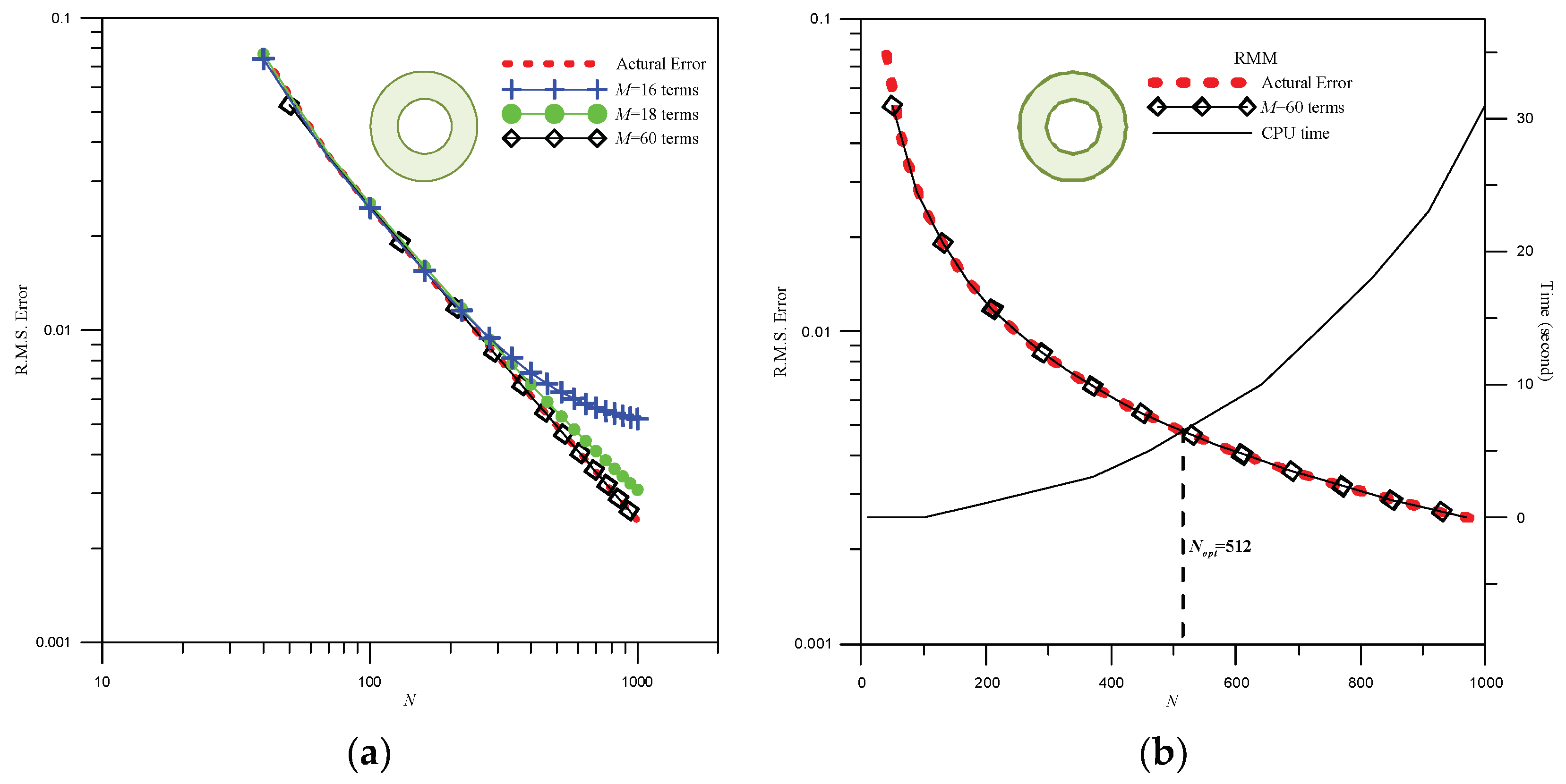
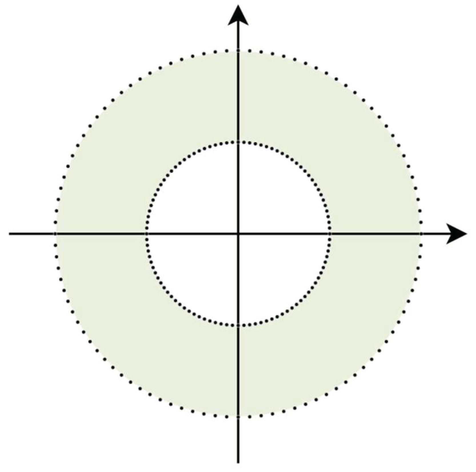
• Case 1: Concentric circles’ domain subjected to Dirichlet B.C.

The problem involving a domain containing concentric circles subjected to Dirichlet B.C. was considered. The wave number $k$ is $\pi$. The exact solution is given by:

$$u=e^{\frac{ik(x+y)}{\sqrt{2}}}.$$

(57)

We define the auxiliary problem and implement the RMM method to solve it. By selecting different values of M in the auxiliary problem, the curves of the R.M.S error for these different values are shown in Figure 3a. The error curve is used as a good indication of the error trend, and it approximates the real error. Referring to Figure 3a, it is evident that M = 60 yields the best results. The convergent analysis of N is illustrated in Figure 3b. After considering both convergent results and CPU time, the optimal number of collocation points is determined to be N_opt = 512 points. The distribution of outer and interior collocation points by adopting N_opt is shown in Figure 4. With the adoption of the optimal number of collocation points, N_opt, the distribution of numerical field solutions is depicted in Figure 5.

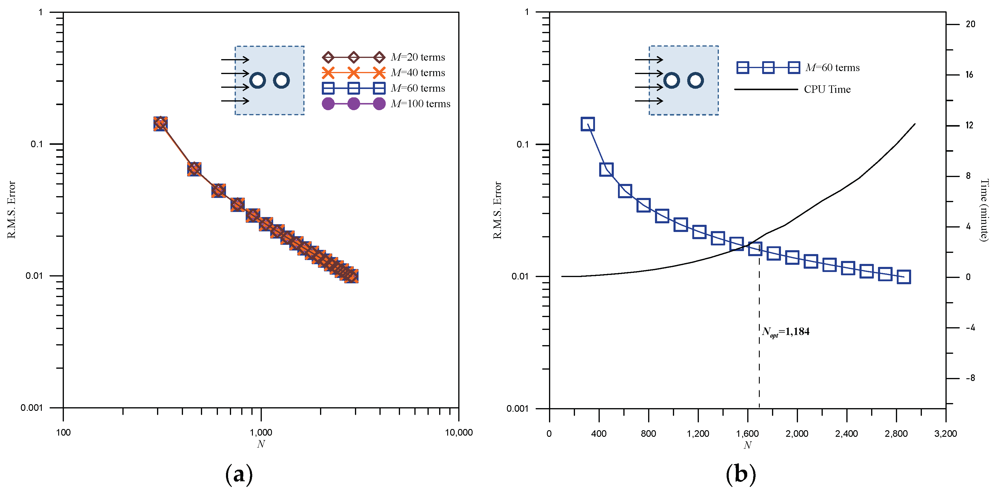
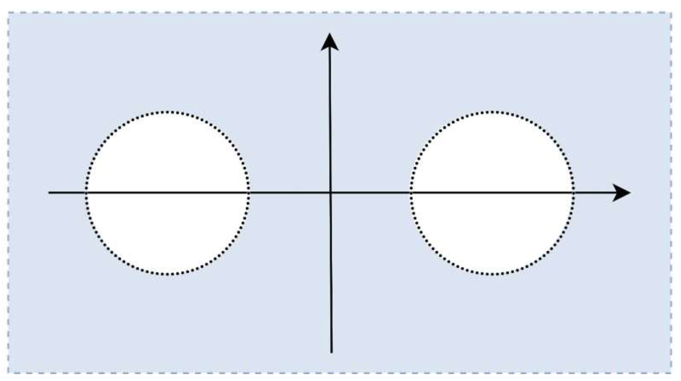
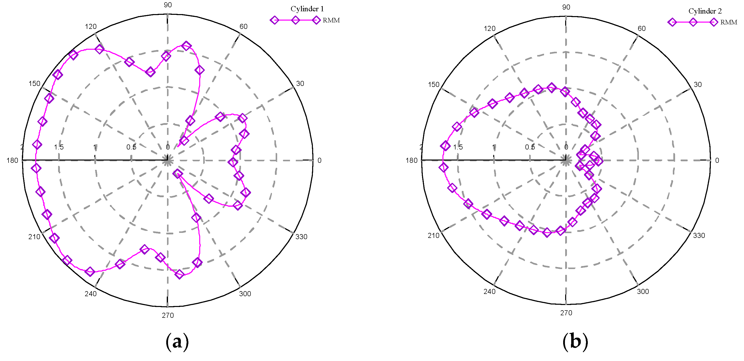
• Case 2: Water wave past two vertical cylinders

The problem of normal incidence waves through two vertical cylinders was considered, and in this case, the wave number $k$ is set to $\pi$. The results of the convergence analysis are depicted in Figure 6. In Figure 6a, the convergence analysis for different values of M using the RMM is presented. Notably, there is no significant difference in the convergence results for different values of M, as observed in Figure 6a. In our experience, M = 60 can be considered suitable. The convergence analysis for the optimal number of collocation points, N, is depicted in Figure 6b. In conjunction with the CPU time curve, N_opt = 1154 can be determined. The distribution of outer and interior collocation points by adopting N_opt for Case 2 is plotted in Figure 7. The free surface elevation results around the left and right cylinders are illustrated in Figure 8a,b, respectively. The maximum elevation of the free surface occurs at 180° for the left cylinder. The resultant force results for different values of kr using the RMM are presented in Figure 9. The results indicate that the resultant force on the left cylinder is greater than that on the right cylinder.

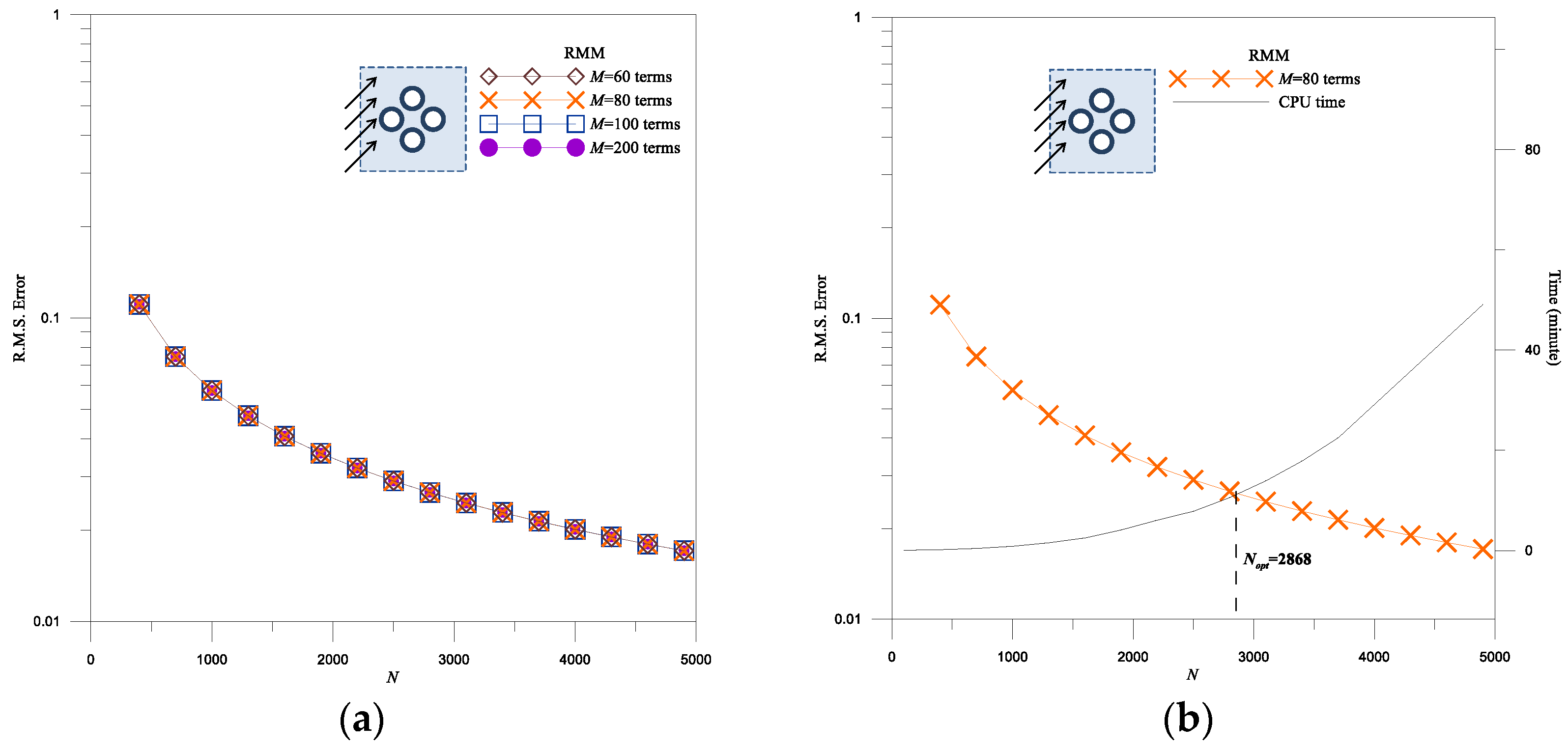
• Case 3: Water wave past four vertical cylinders

In this case, the RMM will be utilized to solve the wave problem involving four vertical cylinders. The numerical results will be compared with those reported in the literature [25]. The wave number k is 4.03482. Two incident angles, ${\theta }_{inc}=0$ and $\pi /2$, are considered.

First, the incident angle ${\theta }_{inc}=0$ was considered. The convergence analysis using the proposed method is illustrated in Figure 10. As seen in Figure 10a, it is evident that the error curve converges when M = 100. Figure 10b displays the curve for the number of collocation points, N, and CPU time. The optimal number of collocation points, N_opt = 2880, can be determined. The distribution of outer and interior collocation points by adopting N_opt for Case 3 is shown in Figure 11. With the parameters mentioned above, we can calculate free surface elevation around different cylinders using the RMM. The results are shown in Figure 12a–d. The maximum wave elevation occurs in the front of the left, top, and bottom cylinders, while the wave elevation is small in the rear of the left, top, and bottom cylinders. The results of resultant force on the corresponding cylinder are plotted in Figure 13a,b. The resultant force results of D.V. Evans [25] are shown in Figure 13a. A noticeable peak near kr = 4 is evident in the Evans result; however, the peak is less pronounced in the RMM result, as shown in Figure 13b. Nevertheless, the results for other kr values exhibit good agreement.

Finally, the angle of the incident wave becomes ${\theta }_{inc}=\pi /2$. The convergence analysis of M and N are shown in Figure 14a,b, respectively. According to Figure 14a, there is little difference in the convergence curves, and we chose M = 80 for the analysis. The analysis of the optimal number of collocation points is shown in Figure 14b. The optimal number of collocation points is N_opt = 2868. Figure 15 shows the elevation of free surface on each cylinder. It can be observed that the position of the maximum wave elevation has changed. Employing the regularization technique of subtraction and addition and selecting the double-layer potential as the basis function results in several disadvantages. The main drawback is that its accuracy is typically limited. Its accuracy slowly improves from ${10}^{-1}$ to ${10}^{-4}$ as the number of points increases. Furthermore, an excessive number of source points do not significantly improve the calculation accuracy. Therefore, establishing an objective criterion for the optimal number of collocation points is important. By combining error estimation techniques, we have achieved a satisfactory result.

5. Conclusions

In this paper, we employ the RMM method combined with the error estimation technique to address the challenge of waves passing multiple cylinders. The approach of combining the RMM with the error estimation technique yields a convergent result that closely approximates the analytical solution. The optimal parameters of the numerical method can be determined through this error estimation technique. Numerical results demonstrate that the optimal number of collocation points for the RMM can be easily determined using the developed error estimation technique, especially when an exact solution is unattainable. A comparison with analytical solutions reveals a close agreement in Case 1. In conclusion, the numerical examination successfully validates the accuracy of the error estimation technique, underscoring its robust predictive capability.

References

1. Chen, J.T.; Kao, J.H.; Huang, Y.L.; Kao, S.K. Applications of degenerate kernels to potential flow across circular, elliptical cylinders and a thin airfoil. Eur. J. Mech. B Fluids 2021, 90, 29–48. [Google Scholar] [CrossRef]
2. Chen, J.T.; Chou, Y.T.; Kao, J.H.; Lee, J.W. Analytical solution for potential flow across two circular cylinders using the BIE in conjunction with degenerate kernels of bipolar coordinates. Appl. Math. Lett. 2022, 132, 108137. [Google Scholar] [CrossRef]
3. Huang, J.; Fan, C.-M.; Chen, J.-H.; Yan, J. Meshless generalized finite difference method for the propagation of nonlinear water waves under complex wave conditions. Mathematics 2022, 10, 1007. [Google Scholar] [CrossRef]
4. Naeem, M.; Yasmin, H.; Shah, R.; Shah, N.A.; Nonlaopon, K. Investigation of fractional nonlinear regularized long-wave models via novel techniques. Symmetry 2023, 15, 220. [Google Scholar] [CrossRef]
5. Chen, K.H.; Hsu, Y.H.; Kao, J.H. Application of the error estimation technique in the method of fundamental solutions for solving incident wave problem with multiple cylinders. Ocean Eng. 2023, 280, 114608. [Google Scholar] [CrossRef]
6. Singh, R.S. Estimation of error variance in linear regression models with errors having multivariate student-t distribution with unknown degrees of freedom. Econ. Lett. 1988, 27, 47–53. [Google Scholar] [CrossRef]
7. Liu, X.; Zheng, S.; Feng, X. Estimation of error variance via ridge regression. Biometrika 2020, 107, 481–488. [Google Scholar] [CrossRef]
8. Wang, X.; Kong, L.; Wang, L. Estimation of error variance in regularized regression models via adaptive lasso. Mathematics 2022, 10, 1937. [Google Scholar] [CrossRef]
9. Guo, Y.; Jacob, B. Estimating the error variance in a high-dimensional linear model. Biometrika 2019, 106, 533–546. [Google Scholar] [CrossRef]
10. Guha Majumdar, S.; Rai, A.; Mishra, D.C. Estimation of error variance in genomic selection for ultrahigh dimensional data. Agriculture 2023, 13, 826. [Google Scholar] [CrossRef]
11. Hon, Y.C.; Chen, W. Boundary knot method for 2D and 3D Helmholtz and the convection-diffusion problems with complicated geometry. Int. J. Numer. Methods Eng. 2003, 56, 1931–1948. [Google Scholar] [CrossRef]
12. Chen, W.; Hon, Y.C. Numerical investigation on convergence of boundary knot method in the analysis of homogeneous Helmholtz, modified Helmholtz, and convection–diffusion problems. Comput. Methods Appl. Mech. Eng. 2003, 192, 1859–1875. [Google Scholar] [CrossRef]
13. Chen, W.; Tanaka, M. A meshfree integration-free and boundary-only RBF technique. Comput. Math. Appl. 2002, 43, 379–391. [Google Scholar] [CrossRef]
14. Jin, B.; Chen, W. Boundary knot method based on geodesic distance for anisotropic problems. J. Comput. Phys. 2006, 215, 614–629. [Google Scholar] [CrossRef]
15. Chen, W. Meshfree boundary particle method applied to Helmholtz problems. Eng. Anal. Bound. Elem. 2002, 26, 577–581. [Google Scholar] [CrossRef]
16. Chen, J.T.; Kao, S.K.; Lee, W.M.; Lee, Y.T. Eigensolutions of the Helmholtz equation for a multiply connected domain with circular boundaries using the multipole Trefftz method. Eng. Anal. Bound. Elem. 2009, 34, 463–470. [Google Scholar] [CrossRef]
17. Kupradze, V.D.; Aleksidze, M.A. The method of functional equations for the approximate solution of certain boundary value problems. USSR Comput. Math. Math. Phys. 1964, 4, 199–205. [Google Scholar] [CrossRef]
18. Fairweather, G.; Karageorghis, A. The method of fundamental solutions for elliptic boundary value problems. Adv. Comput. Math. 1998, 9, 69–95. [Google Scholar] [CrossRef]
19. Cheng, A.H.D.; Young, D.L.; Tsai, C.C. The solution of Poisson’s equation by iterative DRBEM using compactly supported, positive definite radial basis function. Eng. Anal. Bound. Elem. 2000, 24, 549–557. [Google Scholar] [CrossRef]
20. Poullikkas, A.; Karageorghis, A.; Georgiou, G. Methods of fundamental solutions for harmonic and biharmonic boundary value problems. Comput. Mech. 1998, 21, 416–423. [Google Scholar] [CrossRef]
21. Young, D.L.; Chen, K.H.; Lee, C.W. Novel meshless method for solving the potential problems with arbitrary domain. J. Comput. Phys. 2005, 209, 290–321. [Google Scholar] [CrossRef]
22. Hwang, W.S.; Hung, L.P.; Ko, C.H. Non-singular boundary integral formulations for plane interior potential problems. Int. J. Numer. Methods Eng. 2002, 53, 1751–1762. [Google Scholar] [CrossRef]
23. Tournour, M.A.; Atalla, N. Efficient evaluation of the acoustic radiation using multipole expansion. Int. J. Numer. Methods Eng. 1999, 46, 825–837. [Google Scholar] [CrossRef]
24. Chen, K.H.; Kao, J.H.; Chen, J.T. Regularized meshless method for antiplane piezoelectricity problems with multiple inclusions. Comput. Model. Eng. Sci. 2009, 9, 253–279. [Google Scholar]
25. Evans, D.V.; Porter, R. Near-trapping of waves by circular arrays of vertical cylinders. Appl. Ocean Res. 1997, 19, 83–99. [Google Scholar] [CrossRef]
26. Linton, C.M.; Evans, D.V. The interaction of waves with arrays of vertical circular cylinders. J. Fluid Mech. 1990, 215, 549–569. [Google Scholar] [CrossRef]
27. Chen, J.P.; Huang, C.X.; Chen, K.H. Determination of spurious eigenvalues and multiplicities of true eigenvalues using the real-part dual BEM. Comput. Mech. 1999, 24, 41–51. [Google Scholar] [CrossRef]
28. Chen, J.T.; Hong, K.H. Review of dual integral representations with emphasis on hypersingular integrals and divergent series. Trans. Amer. Soci. Mech. Eng. 1999, 52, 17–33. [Google Scholar]
29. Young, D.L.; Chen, K.H.; Lee, C.W. Singular meshless method using double layer potentials for exterior acoustics. J. Acous. Soci. Amer. 2006, 119, 96–107. [Google Scholar] [CrossRef] [PubMed]
30. Abramowitz, M.; Stegun, I.A. Handbook of Mathematical Functions with Formulation Graphs and Mathematical Tables; UNT Digital Library: New York, NY, USA, 1972. [Google Scholar]
Figure 1. The internal and exterior boundaries described by the coordinate origin Oo, O1, Oi and Oj, respectively.
Jmse 12 00492 g001
Figure 2. The flowchart for obtaining Nopt.
Jmse 12 00492 g002
Figure 3. The convergence analysis using the RMM for Case 1 includes: (a) convergence analysis of M and (b) convergence analysis of N.
Jmse 12 00492 g003
Figure 4. The distribution of outer and interior collocation points by adopting Nopt for Case 1.
Jmse 12 00492 g004
Figure 5. The distribution of the field solution for Case 1 using M = 60, N = 512.
Jmse 12 00492 g005
Figure 6. The convergence analysis of wave passing two circular cylinder using the RMM for Case 2; (a) convergence analysis of M, (b) convergence analysis of N.
Jmse 12 00492 g006
Figure 7. The distribution of outer and interior collocation points by adopting Nopt for Case 2.
Jmse 12 00492 g007
Figure 8. The results of free surface elevation around different cylinders for Case 2 using the RMM; (a) around cylinder 1 (left cylinder), (b) around cylinder 2 (right cylinder).
Jmse 12 00492 g008
Figure 9. The resultant force on the corresponding cylinder for Case 2 using the RMM.
Jmse 12 00492 g009
Figure 10. The convergence analysis for different M and N using the RMM. (a) Convergence analysis for M; (b) convergence analysis for N.
Jmse 12 00492 g010
Figure 11. The distribution of outer and interior collocation points by adopting Nopt for Case 3.
Jmse 12 00492 g011
Figure 12. The results of free surface elevation around different cylinders for θ i n c = 0 , (a) cylinder 1 (left); (b) cylinder 2 (top); (c) cylinder 3 (right); (d) cylinder 4 (bottom).
Jmse 12 00492 g012
Figure 13. The resultant force on the corresponding cylinder for θ i n c = 0 , (a) D. V. Evans (1997) results [25], (b) RMM results.
Jmse 12 00492 g013
Figure 14. The convergence analysis of different M and N values for θ i n c = π / 2 , (a) convergence analysis for different M values, (b) convergence analysis for different N values.
Jmse 12 00492 g014
Figure 15. The distribution of free surface elevation around different cylinders for θ i n c = π / 2 . (a) Cylinder 1 (left); (b) cylinder 2 (top); (c) cylinder 3 (right); (d) cylinder 4 (bottom).
Jmse 12 00492 g015
Disclaimer/Publisher’s Note: The statements, opinions and data contained in all publications are solely those of the individual author(s) and contributor(s) and not of MDPI and/or the editor(s). MDPI and/or the editor(s) disclaim responsibility for any injury to people or property resulting from any ideas, methods, instructions or products referred to in the content.