The Propagation Velocity and Influences of Environmental Factors of Deterministic Sea Wave Prediction in the Long Crest Wave

Abstract

Ocean waves are one of the leading environmental factors that cause motion of the ocean’s structure. Wave prediction is of great significance for the safety of marine structures. The deterministic sea wave prediction (DSWP) has been focused on because it provided an accurate temporal wave surface. The propagation velocity of wave components is one of the critical problems in DSWP. In this paper, the research of propagation velocity is focused on. The Taylor expansion to wave number is used to prove that the group velocity is the propagation velocity of wave components. The simulated irregular long crest wave data is generated. Utilizing the simulated data, the calculated wave surfaces based on group velocity are consistent with the simulated results. Meanwhile, the comparisons of calculated results based on the group velocity and phase velocity are given. Then, a tank experiment is set to verify the prediction results. To further investigate the prediction performance under different conditions, the influences of environmental factors, including the wind speed, water depth and sea state are analyzed in this paper.

1. Introduction

Sea waves are one of the maximum loads in the ocean, and all marine structures encounter sea waves all the time. Studying waves, especially wave elevation, can help analyze these structures’ motions effectively. For example, the ship motion quiescent period prediction has been an attractive topic in recent years, which includes three aspects: the measurement of the wave field, the prediction of the wave propagating, and ship motion prediction. The wave elevation should be determined first to predict the ship’s motion for tens of seconds ahead or to estimate whether the ship will be in proper operating condition in the next tens of seconds. Furthermore, the expected wave elevation provides the main input to the warning of approaching unsafe relative motions between the vessel and the rig. Wave elevation prediction has numerous applications in [1,2,3,4,5,6,7,8].

Measuring the wave elevation is the preparation for wave prediction. Many measurement technologies have been developed to help measure the wave elevation or wave fields, such as X-band radar [9], and LIDAR [10,11,12]. Another direct measurement device is the wave buoy, which measures the wave elevation by the reaction between the waves and mooring system [13,14]. Through the analysis of the wave observation data, the sea surface is always described as a stochastic process, and some researchers studied its statistical or spectral properties [15,16,17]. For long-term statistical wave prediction, these models can provide accurate significant wave height, the average period, and other statistical values. However, it is difficult to provide refined wave elevation at fixed points in space.

As the demand for accurate wave prediction grows for a variety of offshore operations, the deterministic sea wave prediction (DSWP) based on the phase-resolved prediction method has gradually become the key research field. Corresponding phase-resolved wave simulation models have also been developed, such as the linear wave theory (LWT), the Higher Order Spectral (HOS) theory [18], the Boussinesq equation [19,20,21,22,23,24], the Green-Naghdi (GN) model [25] and others. These wave models have been continuously refined in recent years and have been widely applied. Dutykh and Dias introduced viscous effects into the Boussinesq equation and conducted a detailed analysis of the viscous potential free surface flows in a fluid layer of finite depth in 2007 [19,20]. Dutykh further proposed a new modeling method for viscous potential free surface flow and analyzed in detail the phase and group velocities resulting from the presence of boundary layers in 2009 [21,22]. The supplementation of these theories is of significant importance for enhancing the accuracy of wave simulation in practical scenarios. Meanwhile, Gao et al., taking the harbor as the research subject, employed the Boussinesq equation to conduct detailed analyses of the interactions between focused transient wave groups and the harbor, as well as Bragg resonance reflection, in 2020 and 2021, respectively [23,24]. This has provided a high reference value for the application of the Boussinesq equation in coastal engineering.

As the complexity of wave models increases, in pursuit of more precise simulation results for wave surfaces, Computational Fluid Dynamics (CFD) methods have gradually evolved, including Smoothed Particle Hydrodynamics (SPH) [26], Finite Volume Method (FVM) [27], and others. Gao et al. carried out the research on the transient gap resonance with consideration of the motion of floating body by using OpenFOAM [28] and Gong et al. simulated the transient fluid resonance phenomenon within the narrow gap between two adjacent boxes, which is excited by incident-focused waves with various spectral peak periods and focused wave amplitudes [29]. These cases demonstrate the good effectiveness of CFD methods in the application of refined flow field and wave field simulation. However, certain boundary conditions can be easily implemented in numerical simulations, yet they are challenging to ascertain in the actual ocean.

Combining the wave model with wave measurement data is an effective method for deterministic wave prediction in real time [30,31]. This method firstly extracts effective wave information from the measured data, such as the frequency and amplitude of wave components. Combining the decomposed wave information with the wave propagation model can achieve the wave reconstruction and prediction in the time–space domain. The linear and nonlinear wave propagation model can be selected according to the designed sea conditions [32,33,34,35,36]. Generally, the nonlinear wave models showed better performance with wave prediction results. However, the computation time also needs to be considered in the wave short-term prediction.

In the process of wave reconstruction and prediction, determining the spatial–temporal predictable zone is a major problem in DSWP. Halliday et al. studied the short-term prediction of sea wave behavior employing the Fast Fourier Transform (FFT) method. They found that the predictable time was limited by the measurement time of wave elevation [1]. However, no method for determining the predictable time was given. Wu studied the predictability of the wave propagation using linear and nonlinear wave models [17]. And this study developed a multi-point measured prediction model aiming to address the limitations of the single-point prediction model. The recent study on DSWP by Naaijen et al. focused on whether the phase or group velocity can indicate the predictable time [37]. They calculated the predictable zone by assessing the energy variation of propagating waves, preliminarily verifying the feasibility of using group velocity as the wave propagation speed but did not provide corresponding theoretical support. Meanwhile, there are many influencing factors for the predictable time for long crest waves, but there are few studies that mention this problem. Edgar et al. [2] considered the maximum predictable time and distances due to the length of the measurement time, water depth and spectral width. Halliday et al. calculated the errors of the FFT-based prediction method at different prediction distances under various wind speeds but did not provide an analysis or explanation of the impact of wind speed on the predictable domain [1]. In conclusion, the selection of propagation velocity is still one of the main problems and the effect of environmental factors needs to be further discussed in DSWP.

In response to the aforementioned issues, this paper firstly presents the reason for selecting group velocity during the wave propagation process using the Taylor expansion of wave numbers, which can provide a theoretical analysis foundation for subsequent related research. Subsequently, this paper conducts a detailed analysis of the consistent zone in time at a fixed point, the consistent zone in space at a specified time, and consistent zone in spacetime, based on the simulated data. Furthermore, this paper carries out the experimental validation and analysis in water tanks. Eventually, catering to the practical engineering application needs, the paper explores and summarizes the predictable time zone of long crest waves under different environmental conditions. We employed different wave spectrums to analyze the impact of factors such as wind speed, water depth, and sea state on the predictable domain, which can offer significant guidance for related marine operations. The rest of this paper is organized as follows: In Section 2, the long-crested wave propagation model is introduced briefly. In Section 3, the consistent zone of the long-crested wave propagation is investigated. The detailed analysis are carried out in Section 4. In Section 5, the water tank experiment is implemented to verify the calculation results. 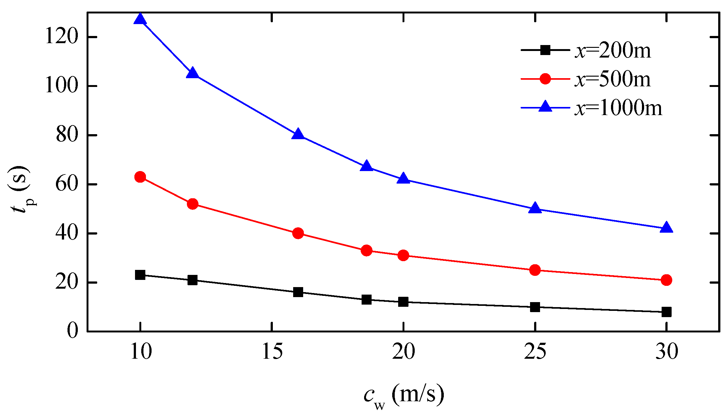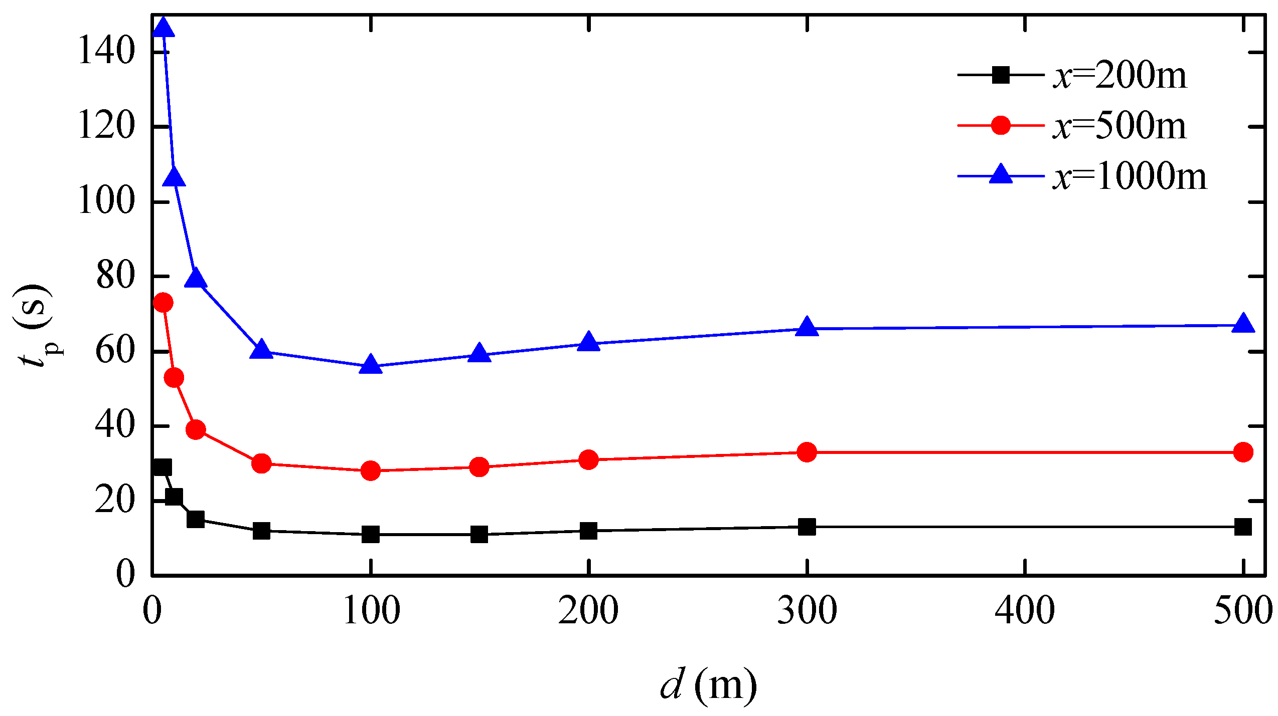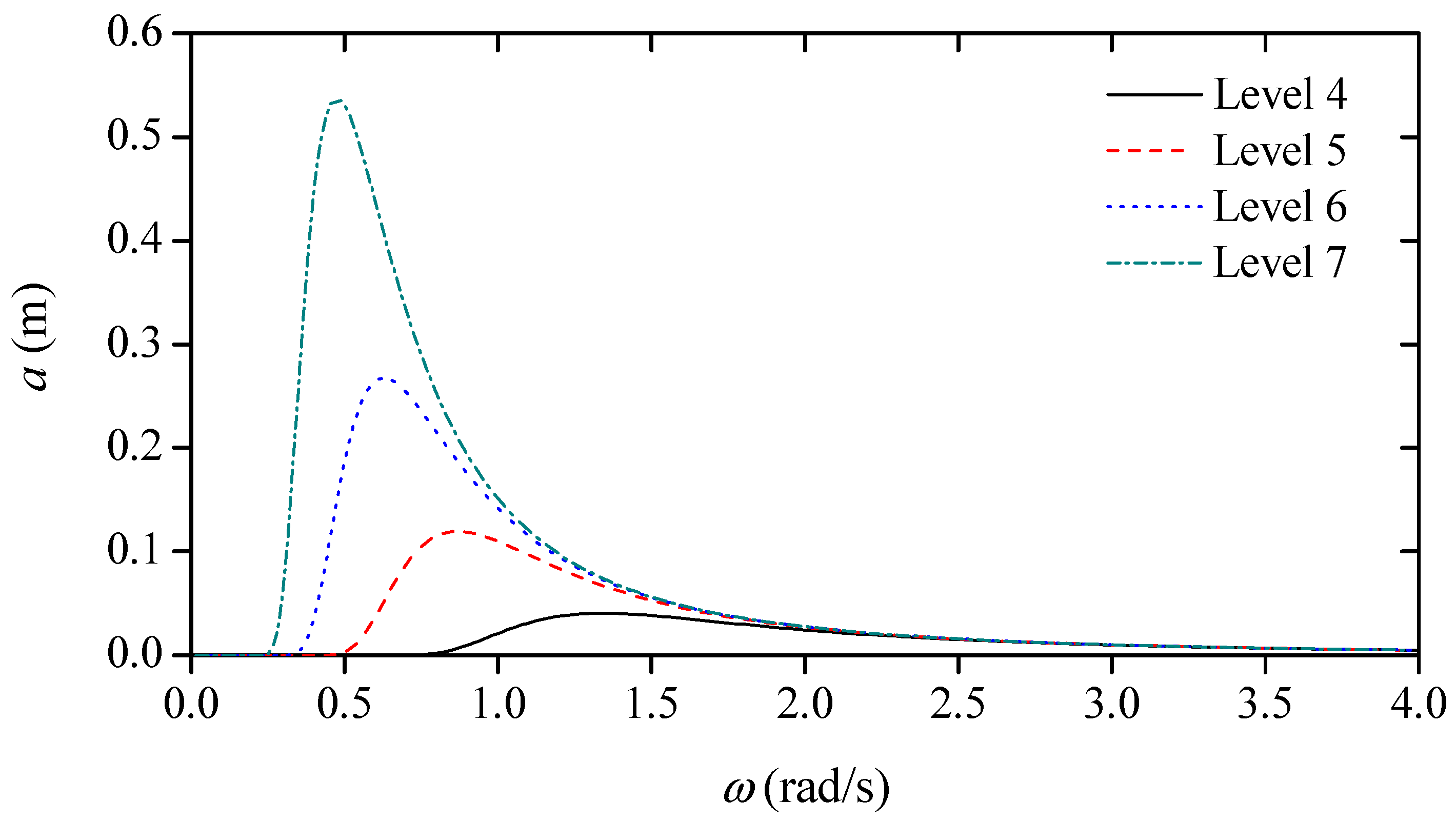In Section 6, a detailed analysis of the factors affecting the predictable time zone is conducted. Finally, discussions and conclusions are explained in Section 7.

2. The Long-Crested Wave Propagation Model

The paper assumes that the sea surface is a stochastic process, and for the two-dimensional case, all wave components propagate in the same direction. Thus, wave elevation with a linear wave model can be used.

$$\eta \left(x,t\right)=\mathrm{Re}\left\{{\displaystyle {\int }_0^{\infty }a\left(\omega \right)e^{i\left[\omega t-k\left(\omega \right)x+\varphi \left(\omega \right)\right]}d\omega }\right\}$$

(1)

where η denotes the wave elevation function of the distance x and time t. The amplitude a, and the wave number k are the functions of the wave angular frequency ω. The initial phase $\varphi$ is selected randomly from 0 to 2π when the wave elevation is given by a known spectrum.

The FFT method is first used to decompose the time series of the wave elevation around the original location into many components and then reconstruct to obtain the wave elevation. Therefore, Equation (1) can be written in a discrete form as follows:

$$\eta \left(x,t\right)={\displaystyle \sum _{i=1}^{N/2}{a}_i\cos \left(w_{i}t-k_{i}x+{\varphi }_i\right)}$$

(2)

where N denotes the number of samples and k can be obtained by the linear dispersion relation as follows:

$${\omega }^2=gk\tanh kh$$

(3)

where g denotes the gravity acceleration and h denotes the water depth. For the infinite water depth case, Equation (3) can be simplified as ω² = gk.

3. Consistent Zone of the Linear DSWP

The consistent zone of the linear DSWP has been preliminary discussed in [2,3]. Firstly, it is necessary to clarify whether the phase or group velocity indicates the consistent time zone and distance zone. When in the deep-water condition, the phase velocity is twice the group velocity, which will cause a noticeable difference on the consistent time zone and distance zone.

3.1. The Propagation Velocity in DSWP

Based on the research in [38], the Taylor expansion to wave number k is used to prove whether the group or phase velocity indicates the consistent time zone and distance zone. Considering the Taylor expansion is used to describe the variation of a function over a small local region, the ocean wave field can be considered as a superposition of many sub-waves of different frequencies. For the sub-waves within a small frequency range from ${\overline{\omega }}^{-}$ to ${\overline{\omega }}^{+}$, it gives the following:

$$\overline{\omega }=\frac{{\overline{\omega }}^{-}+{\overline{\omega }}^{+}}{2}$$

(4)

$$\left|\omega -\overline{\omega }\right|<<1\hspace{1em}\hspace{1em}\omega \in \left[{\overline{\omega }}^{-},{\overline{\omega }}^{+}\right]$$

(5)

where $\overline{\omega }$ is selected as the operational point in order to apply the Taylor expansion for k(ω). Then, the following equation can be obtained:

$$\begin{array}{l}k\left(\omega \right)=\overline{k}+\frac{\partial k}{\partial \omega }\left|{ }_{\omega =\overline{\omega }}\right.\left(\omega -\overline{\omega }\right)+\frac{1}{2!}\frac{{\partial }^{2}k}{\partial {\omega }^2}\left|{ }_{\omega =\overline{\omega }}\right.{\left(\omega -\overline{\omega }\right)}^2+\frac{1}{3!}\frac{{\partial }^{3}k}{\partial {\omega }^3}\left|{ }_{\omega =\overline{\omega }}\right.{\left(\omega -\overline{\omega }\right)}^3+\dots \\ =\overline{k}+\frac{1}{{\overline{c}}_g}\left(\omega -\overline{\omega }\right)+o\left[{\left(\omega -\overline{\omega }\right)}^2\right]\\ =\overline{k}+\frac{1}{{\overline{c}}_g}\left(\omega -\overline{\omega }\right)+R_2\left(\omega \right)\\ \approx \overline{k}+\frac{1}{{\overline{c}}_g}\left(\omega -\overline{\omega }\right) \omega \in \left[{\overline{\omega }}^{-},{\overline{\omega }}^{+}\right]\end{array}$$

(6)

Set $\frac{\partial \omega }{\partial k}\left|{ }_{\omega =\overline{\omega }}\right.={\overline{c}}_g$ as the group velocity of the angular frequency $\overline{\omega }$ and $\overline{k}$ as the wave number of $\overline{\omega }$. R₂(ω) is the second-order Peano remainder term according to Equation (5), which can be omitted.

The wave elevation can be rewritten as follows:

$$\begin{array}{l}\eta \left(x,t\right)=\mathrm{Re}\left\{e^{-i\left[\overline{k}-\frac{\overline{\omega }}{{\overline{c}}_g}\right]x}{\displaystyle {\int }_{{\overline{\omega }}^{-}}^{{\overline{\omega }}^{+}}a\left(\omega \right)e^{i\left[\omega \left(t-\frac{x}{{\overline{c}}_g}\right)+\varphi \left(\omega \right)\right]}d\omega }\right\}\hspace{1em}\hspace{1em}\hspace{1em}t\in \left(-\infty ,\infty \right)\end{array}$$

(7)

At the original location x = x₀, the wave elevation measured from 0 to T can be represented as follows:

$$\begin{array}{l}\varsigma \left(t\right)=\mathrm{Re}\left\{e^{-i\left[\overline{k}-\frac{\overline{\omega }}{{\overline{c}}_g}\right]x_0}{\displaystyle {\int }_{{\overline{\omega }}^{-}}^{{\overline{\omega }}^{+}}a\left(\omega \right)e^{i\left[\omega \left(t-\frac{x_0}{{\overline{c}}_g}\right)+\varphi \left(\omega \right)\right]}d\omega }\right\}\hspace{1em}\hspace{1em}\hspace{1em}t\in \left[0,T\right]\end{array}$$

(8)

It is obvious that with Equation (7), the wave elevation at any location and time (x,t) can be obtained because the sea surface is assumed as a stochastic process. To investigate the limitation of the expected wave elevation at any location and time computed by Equation (8), the comparison between Equations (7) and (8) can indicate the following:

$$\mathrm{Re}\left\{e^{-i\left[\overline{k}-\frac{\overline{\omega }}{{\overline{c}}_g}\right]\left(x-x_0\right)}{\varsigma }_1{\varsigma }_2\left(t-\left(\frac{x-x_0}{{\overline{c}}_g}\right)\right)\right\}=\eta \left(t,x\right)$$

(9)

where:

$$\begin{array}{l}\varsigma \left(t\right)=\mathrm{Re}\left({\varsigma }_1\times {\varsigma }_2\left(t\right)\right)\\ \left\{\begin{array}{l}{\varsigma }_1=e^{-i\left[\overline{k}-\frac{\overline{\omega }}{{\overline{c}}_g}\right]x_0}\\ {\varsigma }_2\left(t\right)={\displaystyle {\int }_{{\overline{\omega }}^{-}}^{{\overline{\omega }}^{+}}a\left(\omega \right)e^{i\left[\omega \left(t-\frac{x_0}{{\overline{c}}_g}\right)+\varphi \left(\omega \right)\right]}d\omega }\end{array}\right.t\in \left[0,T\right]\end{array}$$

(10)

Regarding the left hand of Equation (10), ζ₁ and ζ₂ express the distance and time information, respectively. These two terms are used to obtain the wave elevation from the original location to the target location. Unfortunately, the measurement time is finite. In this case, the time domain of the function ζ is [0, T]. Thus, the time domain of ζ₂ is $\left[\frac{x-x_0}{{\overline{c}}_g},T+\frac{x-x_0}{{\overline{c}}_g}\right]$. The consistent time zone in Equation (8) can be written as

$$T_{pre}\in \left[\frac{x-x_0}{{\overline{c}}_g},T+\frac{x-x_0}{{\overline{c}}_g}\right]\hspace{1em}\hspace{1em}for \overline{\omega }$$

(11)

where T_pre denotes a consistent time zone. When the frequency range from ${\overline{\omega }}^{-}$ to ${\overline{\omega }}^{+}$ is relatively small, it is treated as a regular case and the wave angular frequency is $\overline{\omega }$ and we can describe the coincidence of a regular case as follows: for the measured elevation at the original location x₀ in a time duration T, the beginning of the consistent time zone is the time when the wave reaches x and the end of the consistent time zone is the time when the wave leaves x.

From Equation (9), it is clear to find that the group velocity indicates the consistent time zone and distances zone. Moreover, for irregular cases, the linear wave components can be obtained by FFT and each wave component can be calculated by using Equation (9). Equation (9) is also the basis for building the discrete error function in Section 3.2.

3.2. Discrete Error Function

The classical error function was given by Naaijen et al. [37] and Wu [38]. This error calculation function computes the energy variation in the wave propagation process by discretizing the sub-waves. It evaluates the energy changes during the wave propagation to determine whether the wave can be reconstructed and predicted at the target location and time. The error function calculated at (x,t) can be formulated as follows:

$$\epsilon \left(x,t\right)=\frac{{\displaystyle {\int }_{{\omega }_l}^{{\omega }_h}S\left(\omega \right)d\omega }}{{\displaystyle {\int }_0^{\infty }S\left(\omega \right)d\omega }}$$

(12)

where S(ω) denotes the energy density spectrum, ${\omega }_l$ and ${\omega }_h$ denote the lowest and highest angular frequency for which the energy of the wave component propagated to the target location and time (x,t), respectively.

The relationship between the wave amplitude and energy density is given by the following:

$$a\left(\omega \right)=\sqrt{2S\left(\omega \right)\Delta \omega }$$

(13)

where Δω denotes the frequency step. By using the FFT method, Δω equals to 2π/T.

During the calculation process, the error function needs to be discretized. The discretization of the error function is actually interrelated with the Fourier transform of wave components in the DSWP model. Since the Fourier transform converts an irregular wave time series into a finite number of regular waves, the error function calculation is also based on these discretized regular waves. After the discretization, Equation (12) can be rewritten into a discrete form:

$$\epsilon \left(x,t\right)=\frac{{\displaystyle \sum _{i=1}^M\frac{{\delta }_i{a}_i^2}{2\Delta \omega }}}{{\displaystyle \sum _{i=1}^M\frac{a_i^2}{2\Delta \omega }}}=\frac{{\displaystyle \sum _{i=1}^M{\delta }_i{a}_i^2}}{{\displaystyle \sum _{i=1}^M{a}_i^2}}$$

(14)

The coefficient δ_i (i = 1,2,…,M) can be used to estimate whether the No.i wave component contributes to its elevation or energy. In fact, the linear wave components have already been obtained by the FFT method, as discussed in Section 3.1. δ_i (i = 1,2,…,M) can be evaluated as follows:

$${\delta }_i=\left\{\begin{array}{l}1\hspace{1em}\hspace{1em}t\in \left[\frac{x}{c_i},\frac{x}{c_i}+T\right]\\ 0\hspace{1em}\hspace{1em}else\end{array}\right.$$

(15)

The error function is with respect to the distance x and time t, whose value domain is from 0 to 1. An acceptable error indicator is set as 1 − ε. If 1 − ε equals to 0, it means it coincides at this location and time; if 1 − ε equals to 1, that means it is absolutely unavailable at this location and time. Following Qi [36] and Wu [38], the maximum value of 1 − ε is selected as 0.01. The length of the consistent time zone could be conservative since the maximum value of 1 − ε is relatively small, but it is safer for ocean engineering.

4. Calculation Results Based on Simulated Wave Data

In this section, the irregular waves are simulated to test the accuracy of the statement that group velocity is propagation velocity. The “Original” labeled in the figures means the results generated by the Pierson–Moskowitz spectrum, and “Calculated” means the results calculated via the FFT method. A 12 m/s Pierson–Moskowitz spectrum, in the range of 0–0.5 Hz and with 256 vectors, was used as the input. S(ω) can be written as follows:

$$S\left(\omega \right)=\frac{8.1\times {10}^{-3}{g}^2}{{\omega }^5}\exp \left\{-\frac{0.74g^4}{U^4{\omega }^4}\right\}$$

(16)

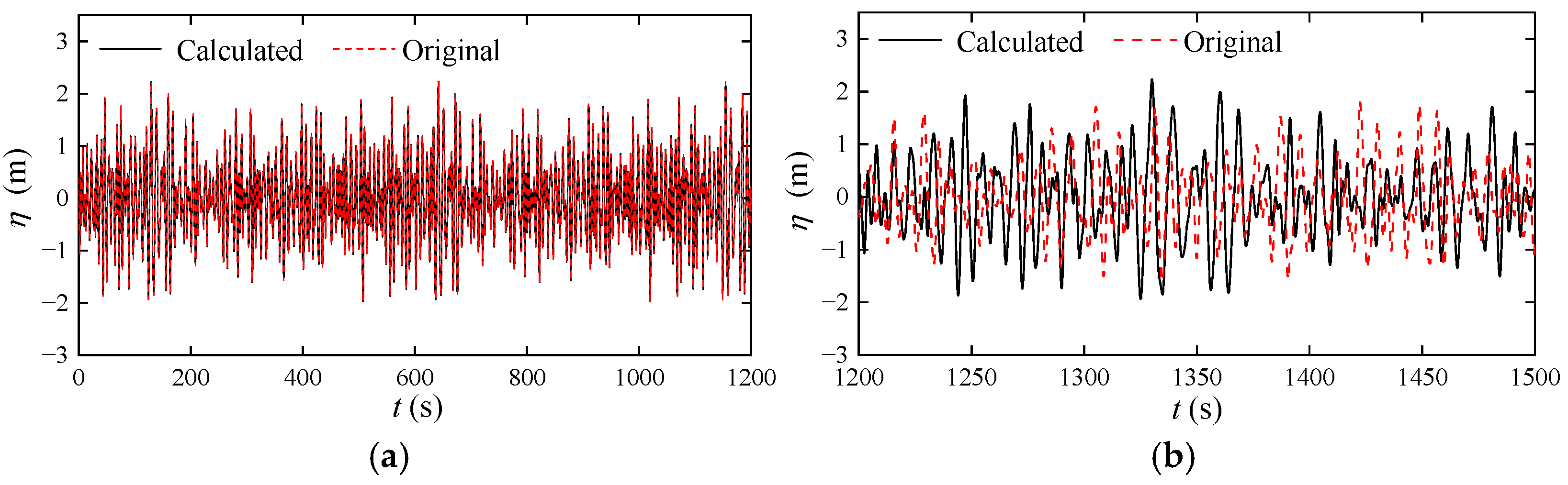
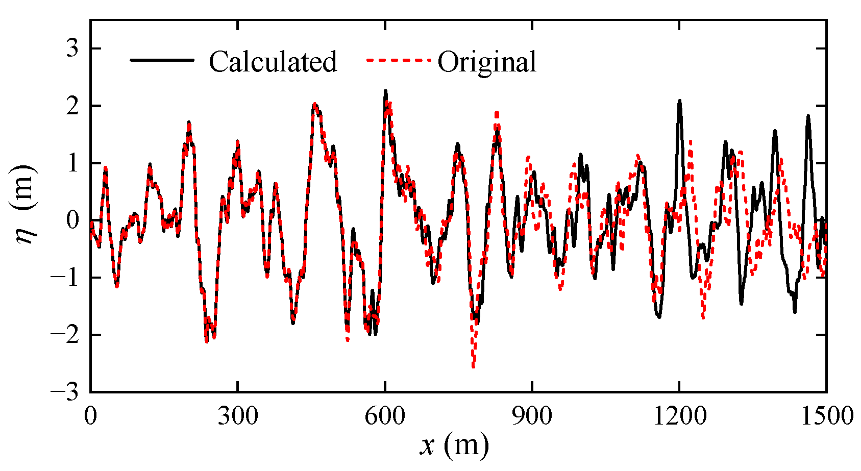
Measurements of the time length of 1200 s with 4096 samples were used to generate the wave elevation at the original location x = 0. The variable measurement time T and the suggested minimum number of N samples were introduced by Halliday et al. [1]. The comparison of the reconstructed and original wave surface from 0 to 1500 s is shown in Figure 1. To provide detailed comparison results in different time ranges, the computational results are divided into two parts, corresponding to Figure 1a for the 0–1200 s and Figure 1b for the 1200–1500 s.

From Figure 1a, it can be seen that the reconstructed wave surface maintains a good trend of variation in comparison with the original wave surface. However, as shown in Figure 1b, when the calculation time exceeds 1200 s, the calculated wave time history curve exhibits noticeable differences from the original wave surface in both amplitude and phase. To further analyze the prediction effect, this paper calculated the Root Mean Square Error (RMSE) for the time history segments of Figure 1a,b, respectively. RMSE is one of the most commonly used errors to measure the degree of fit between time series and the formula is shown in Equation (17) [39].

$$RMSE=\sqrt{\frac{1}{m}{\displaystyle \sum _{i=1}^m{\left(y_i^{calcu}-y_i^{actu}\right)}^2}}$$

(17)

where $y_i^{actu}$ and $y_i^{calcu}$ are the simulated wave elevation and the calculated wave elevation by FFT, respectively; $m$ denotes the number of samples contained within the calculated time segment.

After calculation, the RMSE in Figure 1a is 0.0026, while the RMSE in Figure 1b is as high as 1.0636, which is far greater than the RMSE of Figure 1a. This indicates that the predicted wave surface obtained through FFT transformation at this time has a lower accuracy, and the result is considered unacceptable.

4.1. Wave Surface Consistent Zone in Time

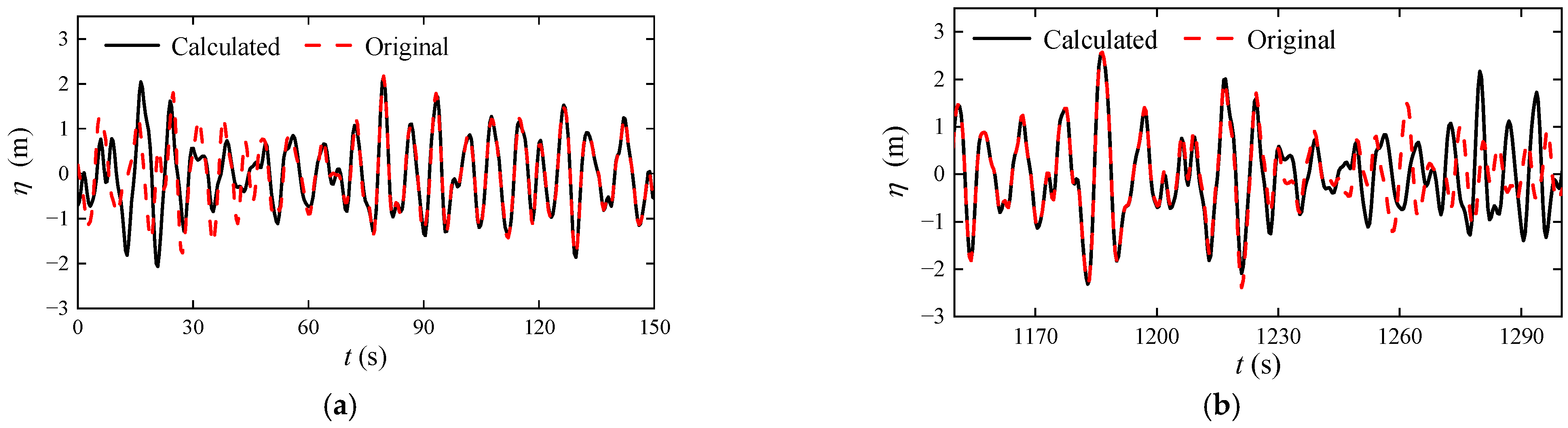
Figure 2 shows the results for the x = 200 m case. The calculation time range is from 0 s to 1300 s. Figure 2a shows the detailed comparison results during 0–150 s and Figure 2b corresponds to 1150–1300 s. It can be seen that the calculated wave elevation and the original elevation of the initial 0~70 s and 1230~1300 s have obvious differences but in the time interval 70~1230 s, the wave surface matches pretty well. Using Equations (12) and (13) to obtain the consistent time zone, the result is shown in Figure 3.

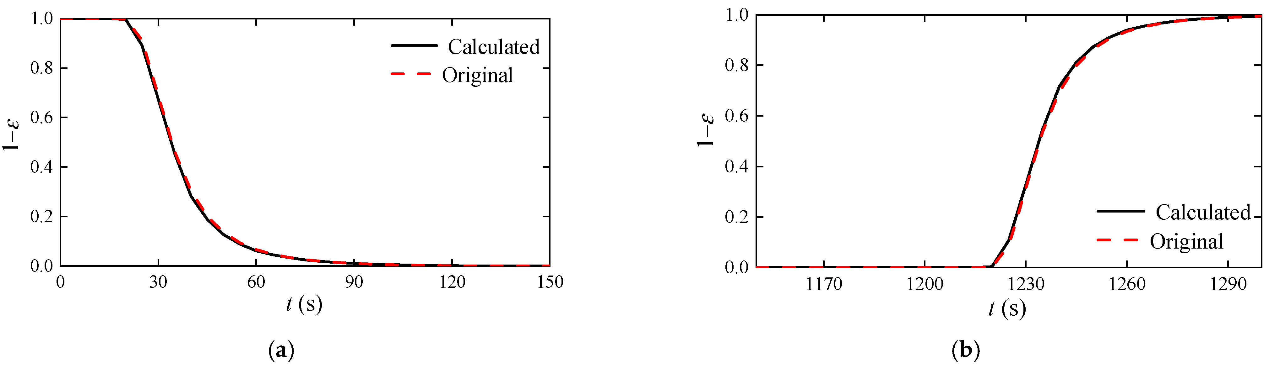
Figure 3 shows the results of the error indicator based on the theoretical spectrum and the FFT components at x = 200 m. Figure 3a,b corresponds to the calculation results in Figure 2a and Figure 2b, respectively. The value of the error indicator by FFT components and the value by the original spectrum matches very well. Since in the natural ocean, the spectrum is unknown, the only information is the measured wave elevation. From Figure 3, we find that the FFT components can give almost the same values of error indicator as the original spectrum. 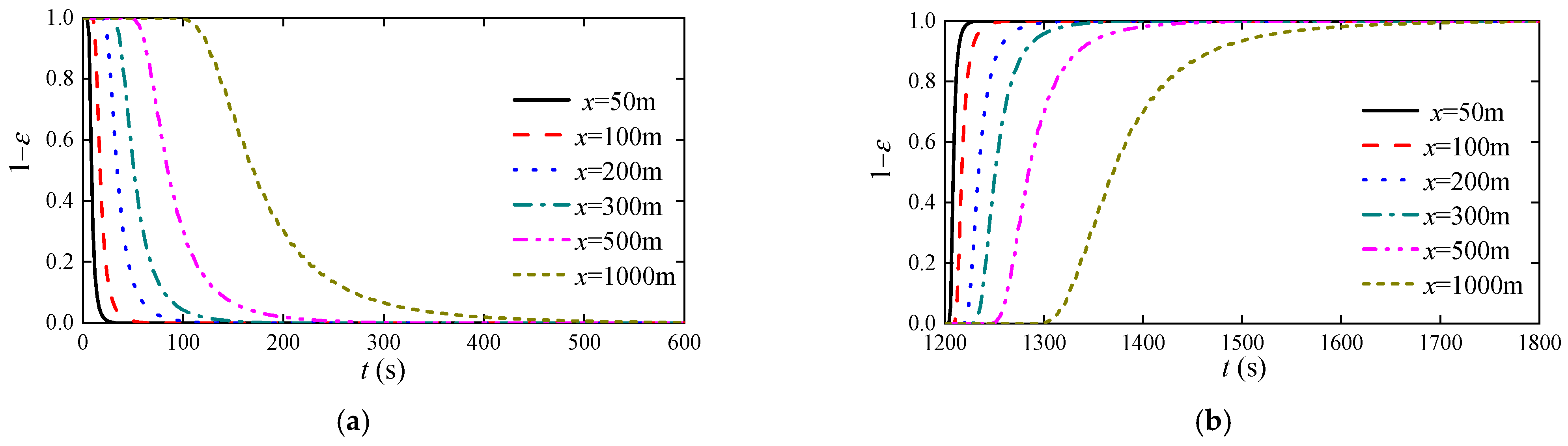Figure 4 shows the time-series results of the error indicator at the different locations. The calculation time range at these locations are all from 0 s to 1800 s. Figure 4a shows the comparison among different locations during 0–150 s and Figure 4b corresponds to 1200–1800 s. These results are calculated based on the group velocity.

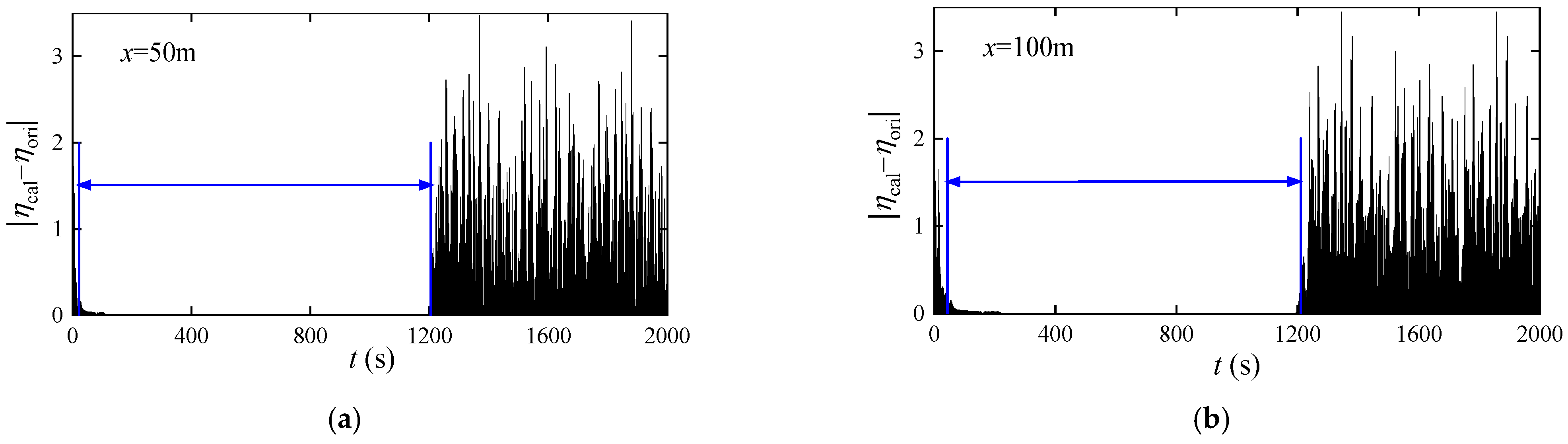
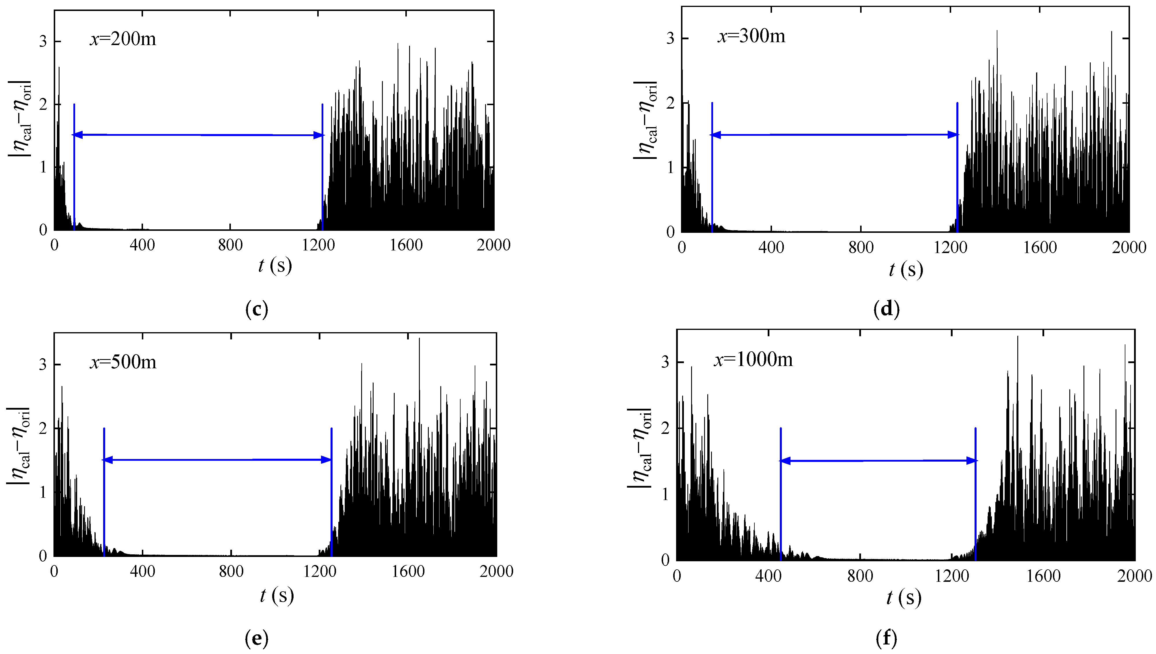
The absolute error function is defined as Equation (18), which can be used to compare the differences between the original elevation and calculated elevation.

$$error\left(x,t\right)=\left|{\eta }_{predicted}\left(x,t\right)-{\eta }_{original}\left(x,t\right)\right|$$

(18)

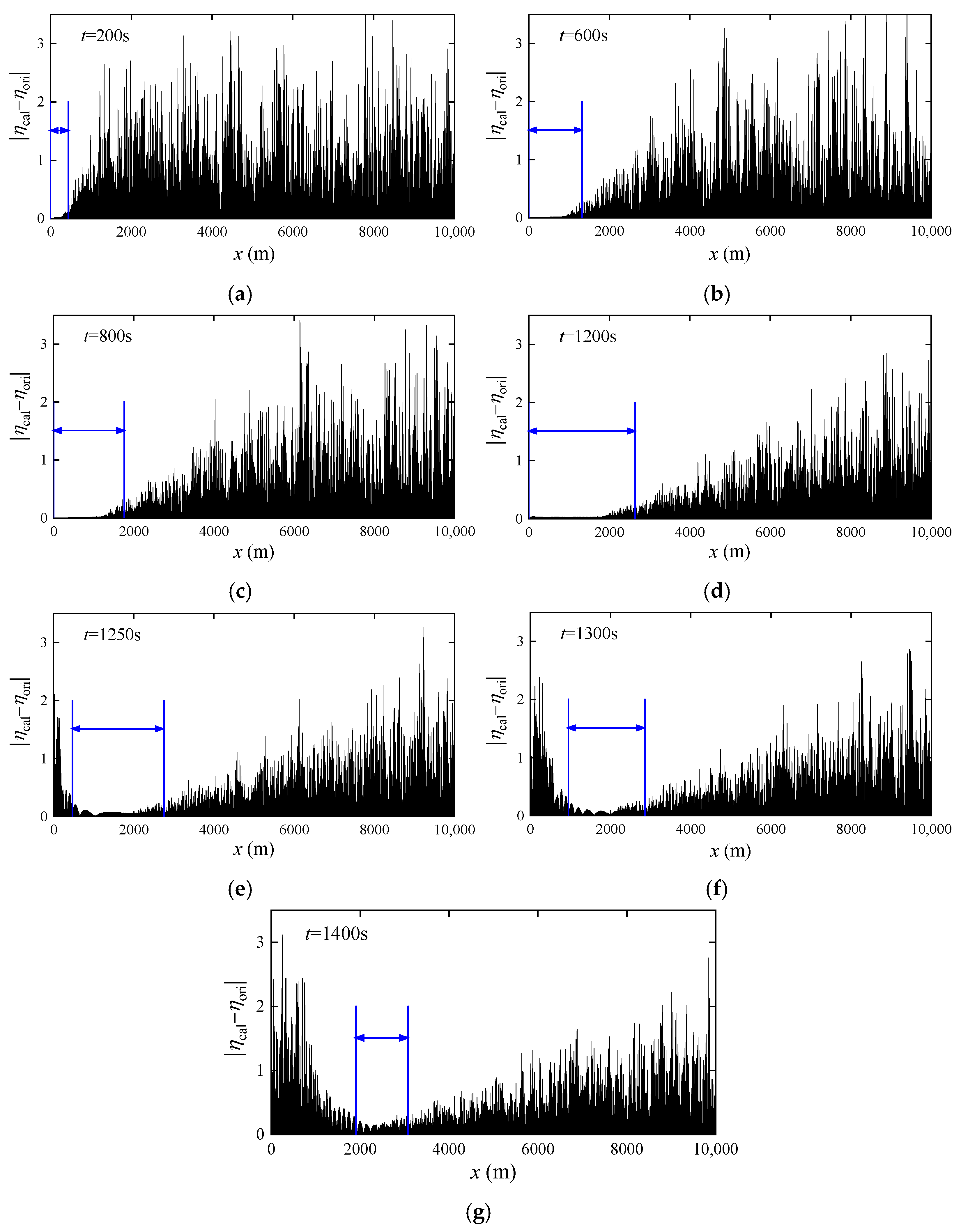
Figure 5 shows the absolute error at different locations. The interval between two blue lines is the consistent time zone obtained by the error function.

Table 1. The consistent time of different locations.

The Distance between Original Location and Target Location (m)	The Beginning of Consistent Time Zone (s)	The End of Consistent Time Zone (s)	The Length of Consistent Time Zone (s)
50	23	1205	1182
100	46	1210	1164
200	92	1221	1129
300	137	1231	1094
500	228	1252	1024
1000	456	1305	849
2000	911	1410	499
2500	1138	1462	224
2608	1187	1473	286
2636	1200	1476	276
3000	1366	1500	144
3500	1457	1512	55

provides the start time and duration of the consistent time zone at different locations. From Figure 5, it can be seen that the distribution of absolute errors is consistent with the calculated predictable domain. The absolute errors of the constructed wave surface in the consistent time zone are significantly lower. Combining with the detailed results shown in Table 1, it can be seen that as the distance between the reconstruction point and the measurement point gradually increases, the consistent time zone also deviates from the initial moment, and the length of the consistent time zone shows a significant decrease. This indicates that distance is an important factor affecting the accuracy of wave reconstruction.

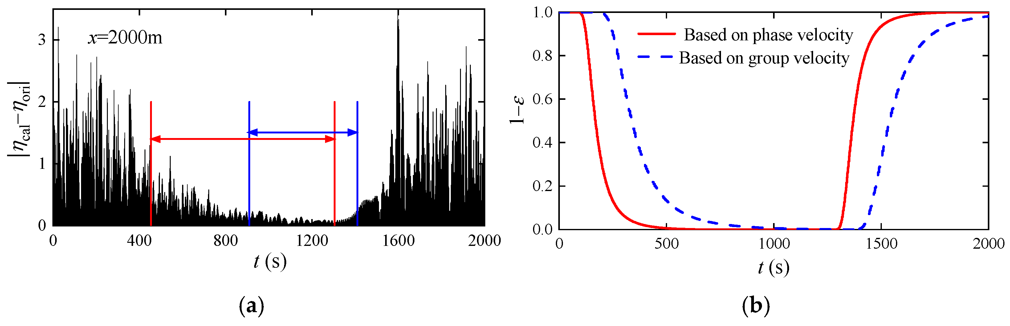
Meanwhile, the consistent time zones obtained by the error function based on group velocity and phase velocity are compared. The target location x = 2000 m is selected to highlight their differences and the result is shown in Figure 6. It can be seen that the error function based on group velocity can provide a consistent time zone rather than that of phase velocity.

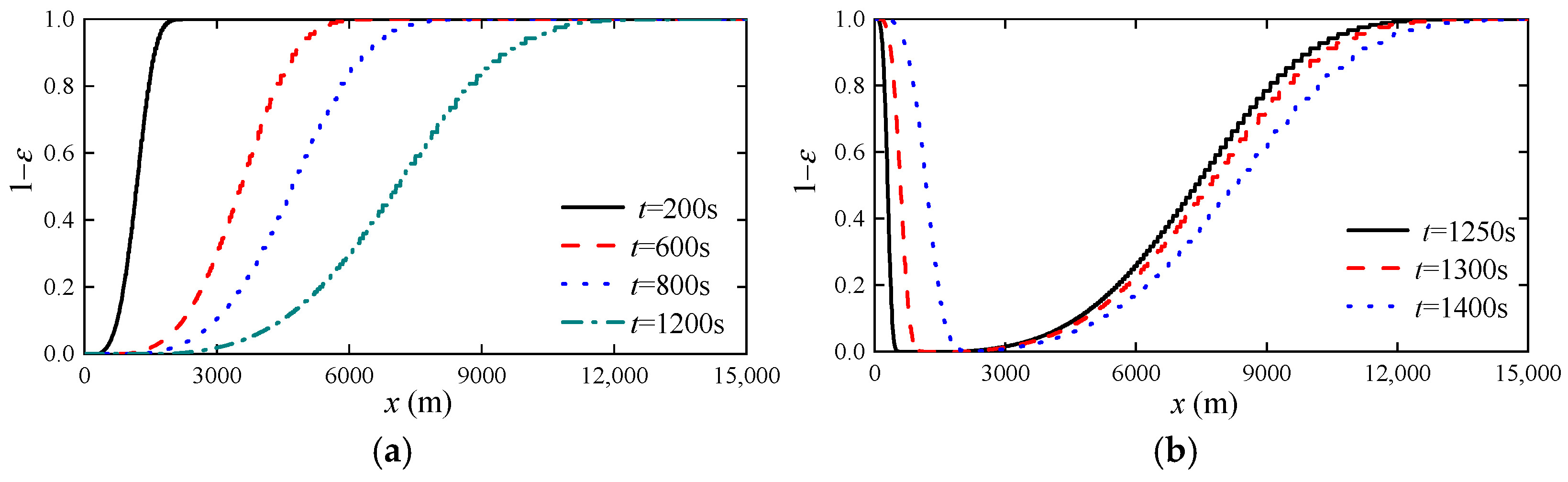
4.2. Wave Surface Consistent Zone in Space

The analysis of the wave surface consistent zone in space selects the fixed time T = 200 s. The comparison between the calculated wave elevation and the original elevation from 0 to 1500 m is shown in Figure 7. For the first 800 m, it can be seen that the calculated wave time history at the current distance matches the original time history quite well, including the prediction of some minor wave surface oscillations and the RMSE is only 0.1896. However, for the next 700 m, there are noticeable differences between the original wave elevation and calculated wave elevation. And the RMSE has increased to 0.8025.

Figure 8 shows the result of the error indicator against distance at different times. To clearly demonstrate the consistent zone in the space of waves at different times, the results shown in Figure 8 are divided into two groups in 1200 s. Before the 1200 s, as shown in Figure 8a, the consistent distance zones are started from the original location and increase with the measurement time. After the 1200 s, the consistent location no longer starts from the original position. Instead, the consistent distance zones appear at locations significantly deviated from the original position.

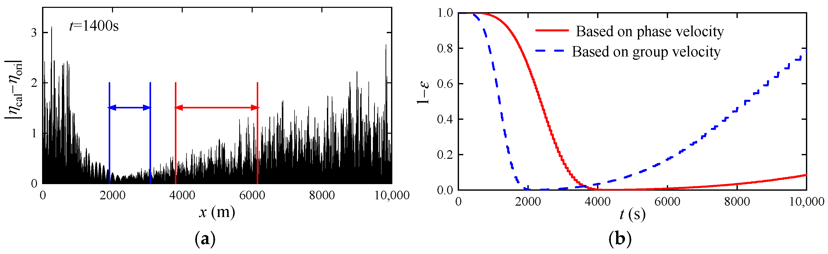
The other six times, including 600 s, 800 s, 1200 s, 1250 s, 1300 s and 1400 s are selected to calculate the absolute error, which is shown in Figure 9. The interval between the two blue lines is the consistent distance zone obtained from the error function. The consistent distance zones shown in Figure 9 are the same as Figure 8, which implies that the calculation of error function can also provide reliable consistent distance zones.

Table 2. The consistent distance zones at different times.

The Moment of Time (s)	The Beginning of Consistent Distance Zone (m)	The end of Consistent Distance Zone (m)	The Length of Consistent Distance Zone (m)
200	0	439	439
600	0	1318	1318
800	0	1757	1757
1200	0	2636	2636
1250	477	2746	2269
1300	953	2856	1903
1400	1905	3076	1171

shows the relationship between the time and consistent distance zone.

Through the simulation results, the consistent distance zones obtained by error function based on group velocity and phase velocity can be also compared. Here the target location T = 1400 s is selected to highlight their differences and the result is shown in Figure 10. It can be observed that the error function based on group velocity can provide a better consistent distance zone rather than that of phase velocity.

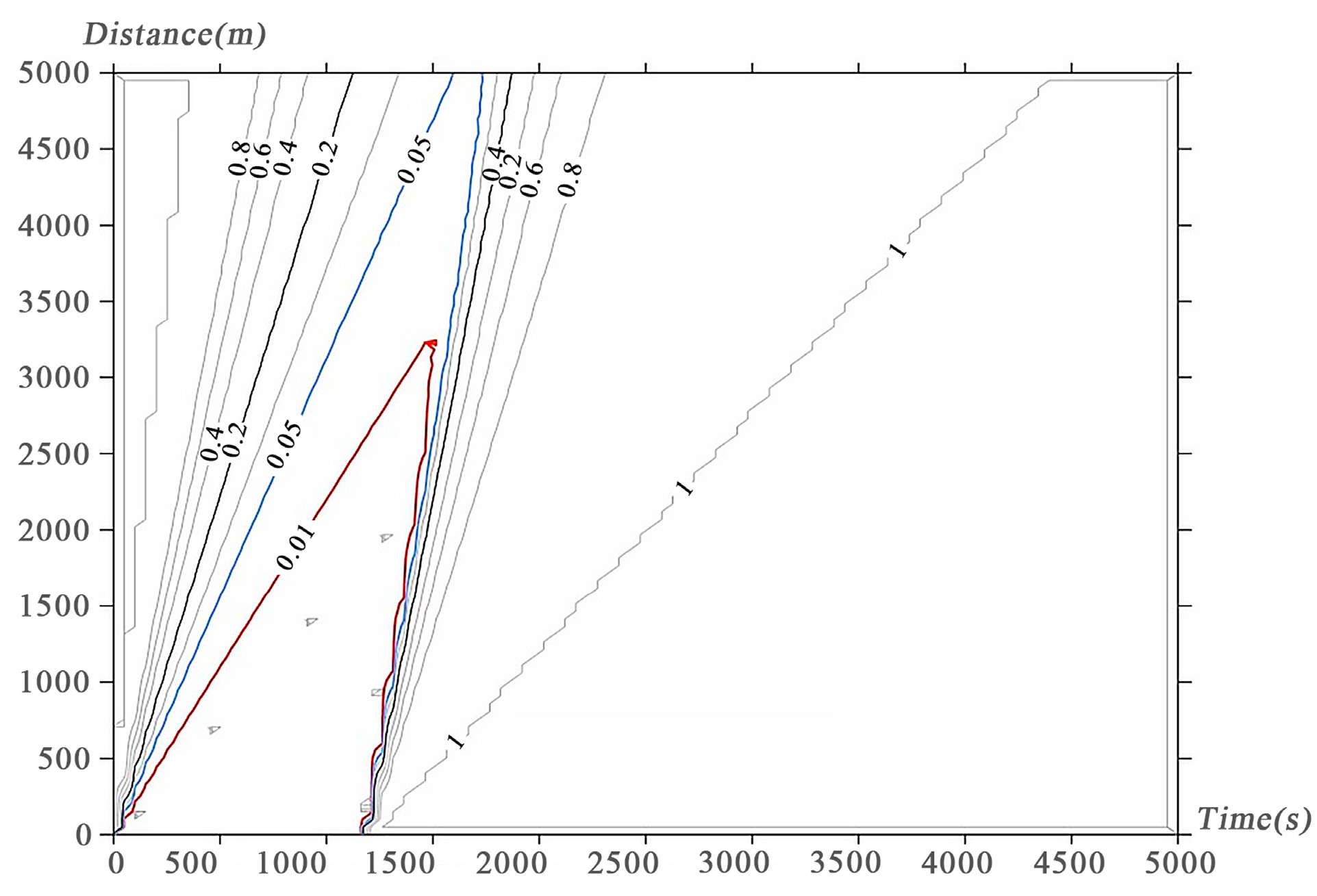
4.3. Wave Surface Consistent Zone in Spacetime

Combining the results of Section 4.1 and Section 4.2, the consistent zone in spacetime can be obtained. The contour of error is showed in Figure 11, and it gives the error in the spacetime coordinate. For any constant error, a closed contour is obtained then. Since the maximum acceptable error is 0.01, the closed area with red lines is consistent with the spacetime zone. The closed area with blue lines is the consistent spacetime zone when the maximum acceptable error is defined as 0.05.

5. Experiments

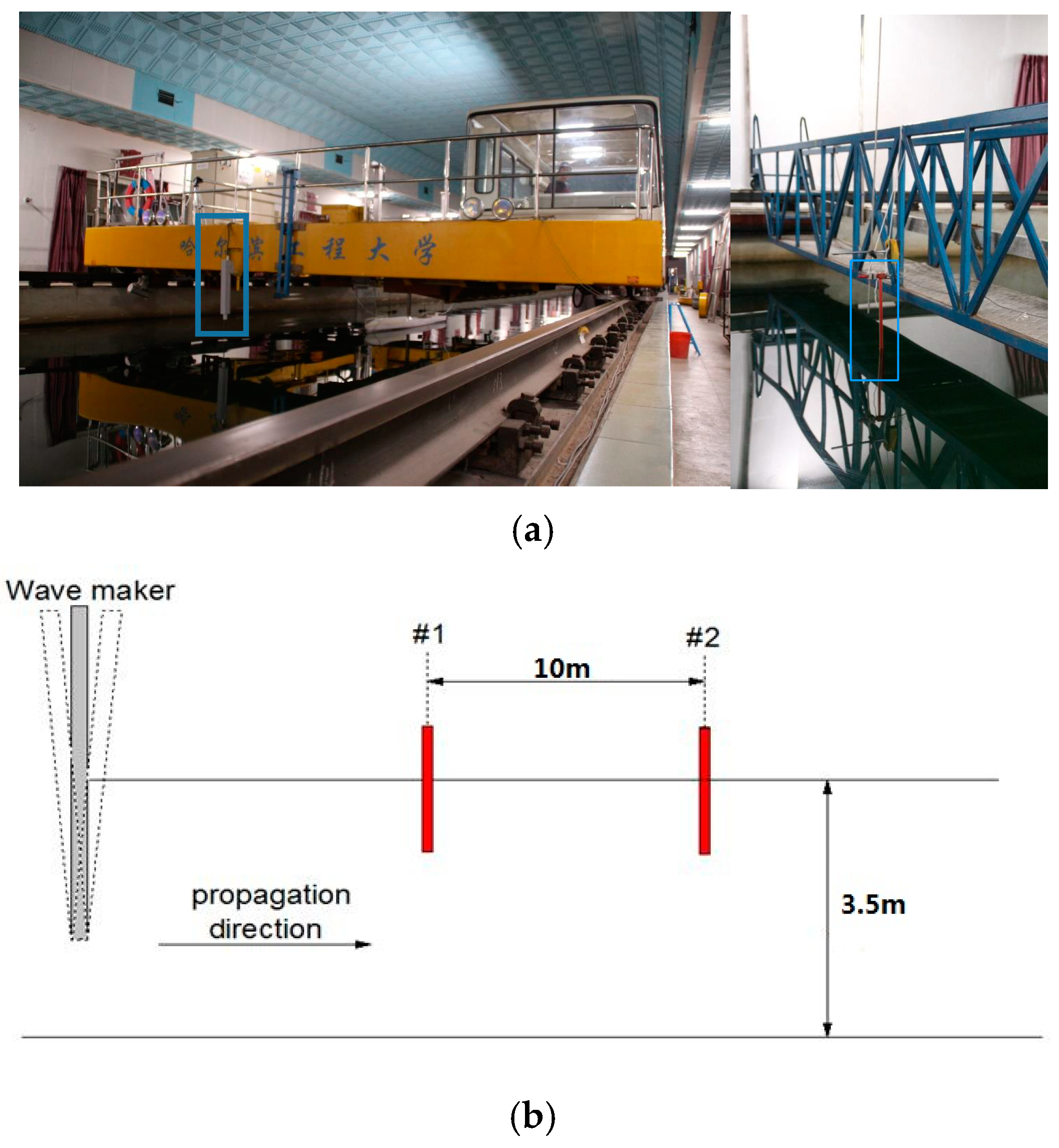
In this section, the experiments are set up in the wave tank of Harbin Engineering University. Figure 12 shows the schematic diagram of the experiments.

Figure 12. The schematic diagram of the experiment (a): The trailer with the “Harbin Engineering University” logo and the placement of the wave gauge. (b): The designed diagram of experiment, where #1 represents the first wave gauge located upstream, and #2 represents the second wave gauge located downstream. Two wave probes are fixed with the distances of 10 m. One wave probe, #1, is used to measure the wave elevation at the original location, and another, #2, is used to measure the wave elevation that will be compared to the estimated wave elevation. When the waves have fully developed and the wave field tends to be stochastic, the wave probes start to measure the wave elevation. To avoid the effect of the wave reflection, the measurement time of all cases is set as 90 s. The sampling frequency is chosen as 0.02 s. The scale radio is selected as 1:64. To generate the irregular waves, the JONSWAP spectrum is selected as the target spectrum. Five cases are chosen for the experiments and the parameters of all cases and the calculated consistent time zones are shown in

Table 3. Parameters of cases.

Case	Significant Wave Height (cm)	Period (s)	Consistent Time Zone (s)
Case 1	3.125	1.25	21~95
Case 2	6.25	1.5	19~94
Case 3	12.5	2	15~93
Case 4	9.375	1.5	18~94
Case 5	9.75	1.25	21~95

.

Figure 12. The schematic diagram of the experiment (a): The trailer with the “Harbin Engineering University” logo and the placement of the wave gauge. (b): The designed diagram of experiment, where #1 represents the first wave gauge located upstream, and #2 represents the second wave gauge located downstream. Two wave probes are fixed with the distances of 10 m. One wave probe, #1, is used to measure the wave elevation at the original location, and another, #2, is used to measure the wave elevation that will be compared to the estimated wave elevation. When the waves have fully developed and the wave field tends to be stochastic, the wave probes start to measure the wave elevation. To avoid the effect of the wave reflection, the measurement time of all cases is set as 90 s. The sampling frequency is chosen as 0.02 s. The scale radio is selected as 1:64. To generate the irregular waves, the JONSWAP spectrum is selected as the target spectrum. Five cases are chosen for the experiments and the parameters of all cases and the calculated consistent time zones are shown in Table 3.

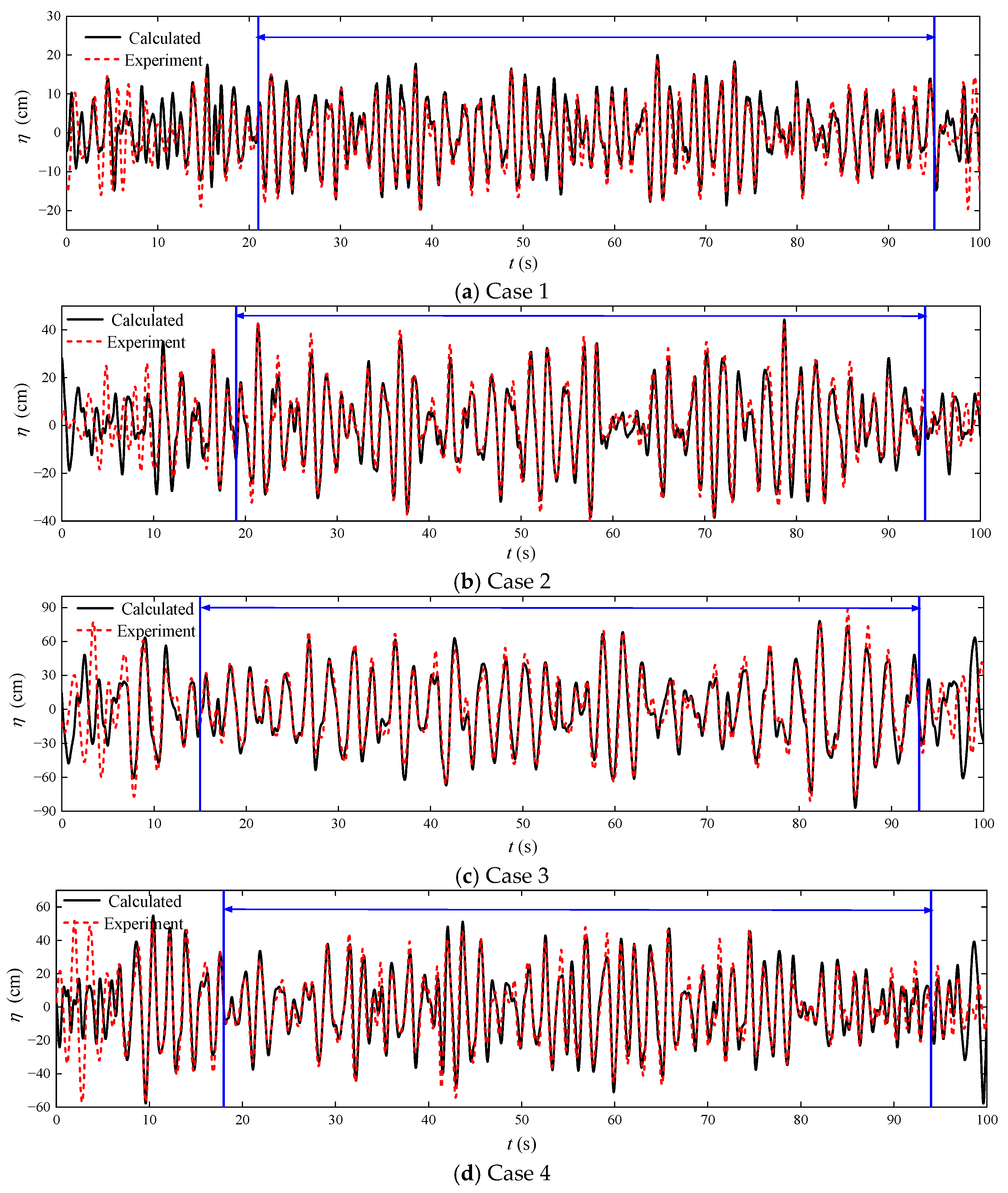
The comparison between the calculated elevation and the measured elevation in the experiment is shown in Figure 13. For each case, the consistent time zone is given and it can be seen that the reconstructed wave surface elevation maintains good consistency with the measured wave surface in both phase and amplitude. However, when beyond the consistent time zone, there will be a noticeable deviation in the reconstructed wave surface elevation. This result indicates that the consistent time zone calculation method provided in this paper is accurate and the consistent time zones could be conservative due to the maximum error of 0.01. Meanwhile, it can be seen that with the increase in wave periods, the length of consistent time zone increases from 74 s (Case 1 and Case 5) to 78 s (Case 3). This is because the propagation and prediction of waves in this paper are calculated based on linear wave theory. Under the linear assumption, the propagation speed of waves is only related to the wave period. When the wave period is longer, the frequency distribution corresponding to the main energy area of the waves will tend towards the low-frequency part, indicating that its constituent sub-waves are more likely to be low-frequency regular waves. Since low-frequency regular waves spread faster, the length of consistent time zone of the waves will decrease.

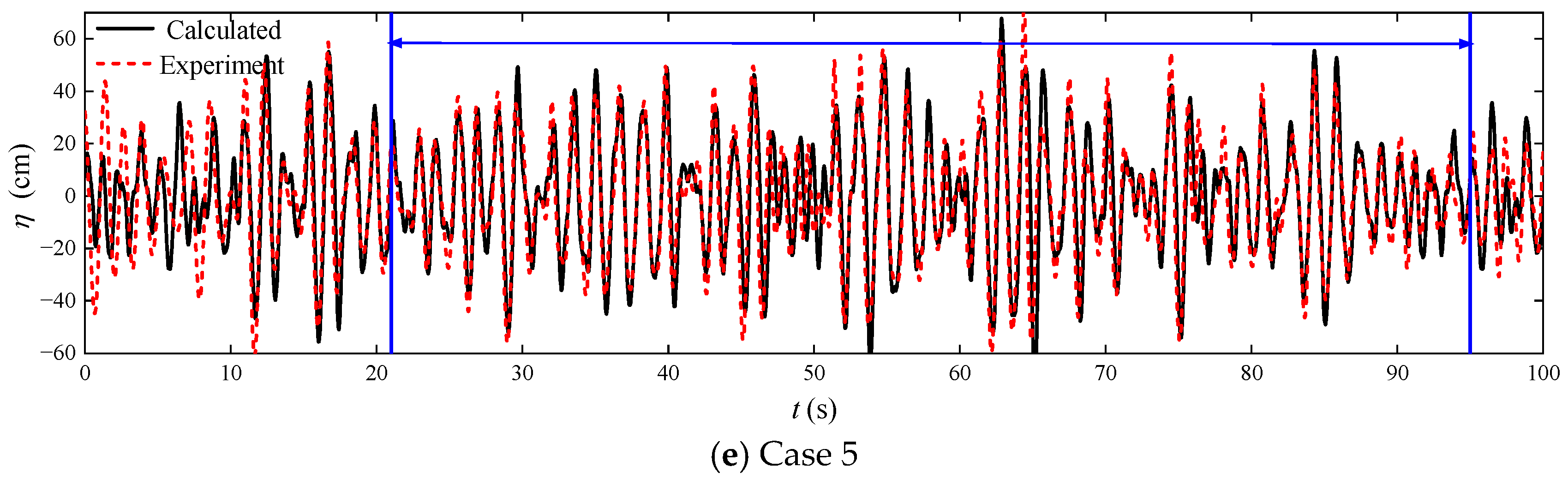
Regarding the consistent time zone, there are some discrepancies between the experimental data and the calculated wave elevation. To investigate the reasons for these differences, four different durations of measured wave elevation from Case 3 are used to calculate the wave elevation for wave probe #2. All four different durations of measured wave elevation can be utilized to determine the consistent time zone interval of 40 to 60 s. As shown in Figure 14, there are approximately no differences among the four calculated elevations. Therefore, the differences between the calculated elevation and experimental data may be attributed to the wave probe measurement error and the minor nonlinearity of the wave tank experiment data. Meanwhile, when using the FFT method, there may be wave energy leakage during the reconstruction process, leading to certain deviations in the reconstruction results. Overall, the calculated results can keep good consistency with the measured wave elevations.

6. Influence Factors for the Predictable Time Zone

The case of irregular waves before is generated by the 12 m/s Pierson–Moskowitz spectrum of the deep-water case. In fact, the wind speed and sea-level usually change under the real sea conditions. Moreover, the offshore structures are usually deployed in shallow water. Therefore, the three influencing factors on the predicted time must be considered for ocean engineering. In this section, the predictable time is defined as the predicted wave elevation after the measurement.

6.1. Wind Speed

Considering the influence of wind speed, seven wind speeds of 10 m/s, 12 m/s, 16 m/s, 18.6 m/s, 20 m/s, 25 m/s and 30 m/s are used in Pierson–Moskowitz spectrum, and the range of 0~0.5 Hz with 256 vectors was used as the input. The measurement time is 1200 s with 4096 samples. Figure 15 shows the comparison of the predictable time with the increasing wind speed of the different locations of 200 m, 500 m and 1000 m.

Figure 15 clearly illustrates that the predictable time decreases as the wind speed increases. Notably, the rate at which the predictable time diminishes tends to slow down with further increments in wind speed. This trend is evident at the specific location x = 1000 m, where the predictable time varies significantly across different wind speeds. For instance, at a wind speed of 10 m/s, the predictable time is 127 s, which is considerably longer compared to the 42 s of predictable time observed at a wind speed of 30 m/s.

To mitigate the impact of varying wind speeds on the accuracy of the predictable time, it is recommended to install a wind speed measurement device on the relevant structure. This addition would enable more precise monitoring and adjustment of the wind speed, thereby enhancing the reliability of the predictable time estimates. By incorporating such a device, the structure can be better prepared for the dynamic changes in wind conditions, leading to improved safety and performance in the face of natural elements.

6.2. Water Depth

To investigate the influence of water depths, nine water depths are selected in the range of 5~500 m. A Pierson–Moskowitz spectrum with 18.6 m/s is selected and the other parameters are kept the same as mentioned in Section 6.1. The wind speed of 18.6 m/s is selected to represent poor winter sea conditions off the west coast of Scotland, following Halliday et al. [1].

Figure 16 shows that with the increase in water depth, the predictable time shows a trend from decline to rise and then it becomes stable, which is caused by the dispersion relation of the finite depth. When the water depth is deep enough, the dispersion relation is close to the case of infinite water depth and the calculated predictable time will keep constant.

6.3. Sea-Level

The ITTC spectrum is selected as the target spectrum to generate irregular waves of different sea-levels. The formula is shown below:

$$S\left(\omega \right)=\frac{8.1\times {10}^{-3}{g}^2}{{\omega }^5}\exp \left\{-\frac{3.11}{{H_{1/3}}^2{\omega }^4}\right\}$$

(19)

The range of frequency domain is 0~4 rad/s with 256 vectors describing all spectrums. The shapes of the amplitude spectrum for four sea-levels are shown in Figure 17.

The measurement time is chosen as 600 s. The calculated predictable time at different distances is shown in

Table 4. Predictable time zone for different sea-levels.

Sea-Level	Significant Wave Height (m)	200 m	500 m	1000 m	2000 m	3000 m
4	0.88	39	98	120–194	Unpredict	Unpredict
5	2.1	25	63	127	Unpredict	Unpredict
6	4	18	46	92	Unpredict	Unpredict
7	7	14	35	70	44–133	Unpredict

.

Table 4 shows the predictable time at different locations. It can be seen that when the sea-level is 4 with the significant wave height of 0.88 m, the distance between the original location and target location is 200 m, and the predictable time is 600~639 s. When the distance is 1000 m, the predictable time zone is 720~794 s. The “Unpredict” means there is no predictable time at this point. Compared with the predictable time under different sea-levels, it can be found that with the sea-level increases, the predictable time decreases for a fixed location. When the sea-level keeps steady, with the distance between the original location and the target location increasing, the predictable time increases and then decreases to 0 gradually.

7. Conclusions

The propagation velocity of DSWP and the influences of environmental factors are studied in this paper. The Taylor expansion to wave number is used to prove that the group velocity is the propagation velocity of wave components. A discrete error function for calculating the consistent time zones and distance zones is defined. A 12 m/s Pierson–Moskowitz spectrum as a target spectrum is used to generate irregular waves in the simulation. The consistent zones of time, space and spacetime are all investigated, and the results show that the method in this paper can accurately obtain consistent time zones and distance zones.

Moreover, the differences of the calculated results based on group velocity and phase velocity are further investigated. The results show that the group velocity can provide good consistent distance zones rather than that of the phase velocity. The results of DSWP methods are verified by the experiments. The influencing factors, including the wind speed, water depth and sea-level of the waves, are considered in this paper. The results show that the predictable time will decrease with higher wind speed or sea-level. With the increase of water depth, the predictable time shows a trend from decline to rise and then it becomes stable.

The detailed analysis of the wave predictable domain can better provide wave prediction information for offshore operations, enhancing the safety of such activities. For instance, during navigation, ships can realize the ship motion prediction by sensing and predicting surrounding waves. The analysis of the wave predictable domain can help to refine the prediction results more effectively. Additionally, as ships navigate through different sea areas, environmental factors such as water depth, wind speed, and sea conditions in the navigational area will change. By integrating the impact analysis of these environmental factors on the wave predictable domain provided in this article, a more precise judgment of the wave predictable domain can be made. This enhances the confidence interval of the predicted results, thereby better ensuring the safety of navigation operations.

It should be noted that the conclusions conducted in this paper are based on linear wave theory. Therefore, when dealing with wave data that exhibits strong nonlinearity, there may be discrepancies between the analysis results of the predictable domain using the methods in this paper. However, the method can still provide a reasonable trend of variation. Nevertheless, nonlinear DSWP models need to be further investigated to achieve accurate nonlinear phase-resolved wave prediction. Meanwhile, in the research concerning the environmental influencing factors on wave propagation, the wave environment under actual sea conditions is more complex. For instance, changes in seafloor topography and variations in water temperature will affect the wave propagation progress. Therefore, conducting detailed studies in specific sea areas based on measured data will be of significance for guiding related offshore operations.

References

1. Halliday, J.R.; Dorrell, D.G.; Wood, A.R. An application of the Fast Fourier Transform to the short-term prediction of sea wave behavior. Renew. Energy 2011, 36, 1685–1692. [Google Scholar] [CrossRef]
2. Edgar, D.R.; Horwood, J.M.K.; Thurley, R.; Belmont, M.R. The effects of parameters on the maximum prediction time possible in short term forecasting of the sea surface shape. Int. Shipbuild. Prog. 2000, 47, 287–301. [Google Scholar]
3. Morris, E.L.; Zienkiewicz, H.K.; Belmont, M.R. Short term forecasting of the sea surface shape. Int. Shipbuild. Prog. 1998, 45, 383–400. [Google Scholar]
4. Riola, J.M.; Diaz, J.J.; Giron-Sierra, J.M. The prediction of calm opportunities for landing on a ship: Aspects of the problem. In Proceedings of the OCEANS 2011 IEEE, Santander, Spain, 6–9 June 2011; pp. 1–8. [Google Scholar]
5. Reichert, K.; Dannenberg, J.; van den Boom, H. X-Band radar derived sea surface elevation maps as input to ship motion forecasting. In Proceedings of the OCEANS′10 IEEE, Sydney, NSW, Australia, 24–27 May 2010; pp. 1–7. [Google Scholar]
6. Naaijen, P.; Huijsmans, R. Real time wave forecasting for real time ship motion predictions. In Proceedings of the International Conference on Offshore Mechanics and Arctic Engineering, Estoril, Portugal, 15–20 June 2008; Volume 48210, pp. 607–614. [Google Scholar]
7. Naaijen, P.; Van Dijk, R.R.T.; Huijsmans, R.H.M.; El-Mouhandiz, A.A. Real time estimation of ship motions in short crested seas. In Proceedings of the International Conference on Offshore Mechanics and Arctic Engineering, Honolulu, HI, USA, 31 May–5 June 2009; Volume 43444, pp. 243–255. [Google Scholar]
8. Hessner, K.; Reichert, K.; Hutt, B.L. Sea surface elevation maps obtained with a nautical X-Band radar—Examples from WaMoS II stations. In Proceedings of the 10th International Workshop on Wave Hindcasting and Forecasting and Coastal Hazard Symposium, North Shore, Oahu, HI, USA, 11–16 November 2007; pp. 11–16. [Google Scholar]
9. Nieto-Borge, J.C.; Mata-Moya, D.; Jarabo-Amores, P.; Reichert, K.; Hessner, K. Application of conventional marine radars for measuring ocean wave fields in shallow water conditions. In Proceedings of the 2010 IEEE International Geoscience and Remote Sensing Symposium, Honolulu, HI, USA, 25–30 July 2010; pp. 4338–4341. [Google Scholar]
10. Nieto Borge, J.C.; RodrÍguez, G.R.Í.; Hessner, K.; González, P.I. Inversion of marine radar images for surface wave analysis. J. Atmos. Ocean. Technol. 2004, 21, 1291–1300. [Google Scholar] [CrossRef]
11. Belmont, M.R.; Horwood, J.M.K.; Thurley, R.W.F.; Baker, J. Shallow angle wave profiling lidar. J. Atmos. Ocean. Technol. 2007, 24, 1150–1156. [Google Scholar] [CrossRef]
12. Desmars, N.; Bonnefoy, F.; Grilli, S.; Ducrozet, G.; Perignon, Y.; Guérin, C.-A.; Ferrant, P. Experimental and numerical assessment of deterministic nonlinear ocean waves prediction algorithms using non-uniformly sampled wave gauges. Ocean. Eng. 2020, 212, 107659. [Google Scholar] [CrossRef]
13. Tucker, M.J.; Pitt, E.G. Waves in Ocean Engineering; Elsevier: Amsterdam, The Netherlands, 2001. [Google Scholar]
14. Krogstad, H.E.; Barstow, S.F.; Aasen, S.E.; Rodriguez, I. Some recent developments in wave buoy measurement technology. Coast. Eng. 1999, 37, 309–329. [Google Scholar] [CrossRef]
15. Belmont, M.R.; Horwood, J.M.K. The effect of frequency distribution in sea model spectra on simulations of deterministic sea wave prediction. Int. Shipbuild. Prog. 1999, 46, 265–276. [Google Scholar]
16. Hao, W.; Sun, X.; Wang, C.; Chen, H.; Huang, L. A hybrid EMD-LSTM model for non-stationary wave prediction in offshore China. Ocean. Eng. 2022, 246, 110566. [Google Scholar] [CrossRef]
17. Pierson, W.J. Practical Methods for Observing and Forecasting Ocean Waves by Means of Wave Spectra and Statistics; Hydrographic Office: Washington, DC, USA, 1958. [Google Scholar]
18. Dommermuth, D.G.; Yue, D.K.P. A high-order spectral method for the study of nonlinear gravity waves. J. Fluid Mech. 1987, 184, 267–288. [Google Scholar] [CrossRef]
19. Dutykh, D.; Dias, F. Dissipative Boussinesq equations. C. R. Mec. 2007, 335, 559–583. [Google Scholar] [CrossRef]
20. Dutykh, D.; Dias, F. Viscous potential free-surface flows in a fluid layer of finite depth. C. R. Acad. Sci. Paris Ser. I 2007, 345, 113–118. [Google Scholar] [CrossRef]
21. Dutykh, D. Visco-potential free-surface flows and long wave modelling. Eur. J. Mech. B/Fluids 2009, 28, 430–443. [Google Scholar] [CrossRef]
22. Dutykh, D. Group and phase velocities in the free-surface visco-potential flow: New kind of boundary layer induced instability. Phys. Lett. A 2009, 373, 3212–3216. [Google Scholar] [CrossRef]
23. Gao, J.L.; Ma, X.Z.; Zang, J.; Dong, G.H.; Ma, X.J.; Zang, J.; Zhou, L. Investigation on the effects of Bragg reflection on harbor oscillations. Coast. Eng. 2021, 170, 103977. [Google Scholar] [CrossRef]
24. Gao, J.L.; Ma, X.Z.; Zang, J.; Dong, G.H.; Ma, X.J.; Zhu, Y.Z.; Zhou, L. Numerical investigation of harbor oscillations induced by focused transient wave groups. Coast. Eng. 2020, 158, 103670. [Google Scholar] [CrossRef]
25. Zhao, B.B.; Duan, W.Y.; Ertekin, R.C.; Hayatdavoodi, M. High-level Green-Naghdi wave models for nonlinear wave transformation in three dimensions. Ocean Eng. Mar. Energy 2015, 1, 121–132. [Google Scholar] [CrossRef]
26. Salis, N.; Hu, X.; Luo, M.; Reali, A.; Manenti, S. 3D SPH analysis of focused waves interacting with a floating structure. Appl. Ocean. Res. 2024, 144, 103885. [Google Scholar] [CrossRef]
27. Liu, C.L.; Sui, T.T.; Zhang, J.S.; Zhang, C. 3D numerical investigation of wave-induced seabed response around a tripod pile foundation with different arrangements. Ocean Eng. 2023, 287, 115861. [Google Scholar] [CrossRef]
28. Gao, J.L.; Lyu, J.; Wang, J.H.; Zhang, J.; Liu, Q.; Zang, J.; Zou, T. Study on Transient Gap Resonance with Consideration of the Motion of Floating Body. China Ocean. Eng. 2022, 36, 994–1006. [Google Scholar] [CrossRef]
29. Gong, S.K.; Gao, J.L.; Mao, H.F. Investigations on fluid resonance within a narrow gap formed by two fixed bodies with varying breadth ratios. China Ocean. Eng. 2023, 37, 962–974. [Google Scholar] [CrossRef]
30. Hlophe, T.; Taylor, P.H.; Kurniawan, A.; Orszaghova, J.; Wolgamot, H. Phase-resolved wave prediction in highly spread seas using optimised arrays of buoys. Appl. Ocean Res. 2023, 130, 103435. [Google Scholar] [CrossRef]
31. Kim, I.-C.; Ducrozet, G.; Leroy, V.; Bonnefoy, F.; Perignon, Y.; Bourguignon, S. A real-time wave prediction in directional wave fields: Strategies for accurate continuous prediction in time. Ocean Eng. 2024, 291, 116445. [Google Scholar] [CrossRef]
32. Duncan, P.E.; Drake, K.R. A note on the simulation and analysis of irregular non-linear waves. Appl. Ocean Res. 1995, 17, 1–8. [Google Scholar] [CrossRef]
33. Blondel, E.; Bonnefoy, F.; Ferrant, P. Deterministic non-linear wave prediction using probe data. Ocean Eng. 2010, 37, 913–926. [Google Scholar] [CrossRef]
34. Blondel, E.; Bonnefoy, F.; Ferrant, P. Experimental validation of deterministic non-linear wave prediction schemes in 2D. In Proceedings of the Twentieth International Offshore and Polar Engineering Conference, Beijing, China, 20–25 June 2010. [Google Scholar]
35. Dalzell, J.F. A note on finite depth second-order wave–wave interactions. Appl. Ocean Res. 1999, 21, 105–111. [Google Scholar] [CrossRef]
36. Qi, Y.; Wu, G.; Liu, Y.; Yue, D.K. Predictable zone for phase-resolved reconstruction and forecast of irregular waves. Wave Motion 2018, 77, 195–213. [Google Scholar] [CrossRef]
37. Naaijen, P.; Trulsen, K.; Blondel-Couprie, E. Limits to the extent of the spatio-temporal domain for deterministic wave prediction. Int. Shipbuild. Prog. 2014, 61, 203–223. [Google Scholar]
38. Wu, G. Direct Simulation and Deterministic Prediction of Large-Scale Nonlinear Ocean Wave-Field. Ph.D. Thesis, Massachusetts Institute of Technology, Cambridge, MA, USA, 2004. [Google Scholar]
39. Chen, H.; Bu, Y.; Zong, K.; Huang, L.; Hao, W. The Effect of Data Skewness on the LSTM-Based Mooring Load Prediction Model. J. Mar. Sci. Eng. 2022, 10, 1931. [Google Scholar] [CrossRef]
Figure 1. The comparison of the calculated and original elevation at the original location. (a): The comparison result from 0 to 1200 s. (b): The comparison result from 1200 s to 1500 s.
Jmse 12 00633 g001
Figure 2. The comparison of calculated and original elevation at x = 200 m. (a): The comparison result from 0 to 150 s. (b): The comparison result from 1150 s to 1300 s.
Jmse 12 00633 g002
Figure 3. The value of the error indicator against time at x = 200 m. (a): The distribution and trend of errors from 0 to 150 s. (b): The distribution and trend of errors from 1150 s to 1300 s.
Jmse 12 00633 g003
Figure 4. The values of error indicator against time at different locations. (a): The error indicator from 0 to 600 s. (b): The error indicator from 1200 s to 1800 s.
Jmse 12 00633 g004
Figure 5. The absolute error against time at different locations. (a): The error calculated at x = 50 m. (b): The error calculated at x = 100 m. (c): The error calculated at x = 200 m. (d): The error calculated at x = 300 m. (e): The error calculated at x = 500 m. (f): The error calculated at x = 1000 m.
Jmse 12 00633 g005aJmse 12 00633 g005b
Figure 6. The comparison of the consistent time zone based on group velocity and phase velocity (a): The comparison of calculated absolute error based on group velocity and phase velocity, which is shown in blue line and red line respectively. (b): The comparison of calculated 1 − ε based on group velocity and phase velocity.
Jmse 12 00633 g006
Figure 7. The comparison of the calculated and original elevation at T = 200 s.
Jmse 12 00633 g007
Figure 8. The value of error indicator against time at different locations. (a): The error indicator at T = 200 s, 600 s, 800 s, 1200 s. (b): The error indicator at T = 1250 s, 1300 s, 1400 s.
Jmse 12 00633 g008
Figure 9. The absolute error against distances at different time. (a): The absolute error calculated at t = 200 s. (b): The absolute error calculated at t = 600 s. (c): The absolute error calculated at t = 800 s. (d): The absolute error calculated at t = 1200 s. (e): The absolute error calculated at t = 1250 s. (f): The absolute error calculated at t = 1300 s. (g): The absolute error calculated at t = 1400 s.
Jmse 12 00633 g009
Figure 10. The comparison of the consistent distance zones based on group velocity and phase velocity (a): The comparison of calculated absolute error based on group velocity and phase velocity, which is shown in blue line and red line respectively. (b): The comparison of calculated 1 − ε based on group velocity and phase velocity.
Jmse 12 00633 g010
Figure 11. The contour plot of error in spacetime. (The lines of different colors represent the contour lines of the consistent zone corresponding to various 1 − ε values. The red, blue, black, and gray lines correspond to the consistent zone contour lines at 1 − ε = 0.01, 1 − ε = 0.05, 1 − ε = 0.2, and 1 − ε > 0.2, respectively. The enclosed area formed by lines represents the consistent zone in spacetime. The triangular area enclosed by the red line indicates the consistent zone in spacetime when 1 − ε < 0.01.)
Jmse 12 00633 g011
Figure 13. Comparison of experiment data and calculated elevation.
Jmse 12 00633 g013aJmse 12 00633 g013b
Figure 14. The calculated wave elevation based on different time intervals of the measurement elevation.
Jmse 12 00633 g014
Figure 15. The comparison of predictable time against wind speed at different locations.
Jmse 12 00633 g015
Figure 16. The variation of predictable time against the water depth at different locations.
Jmse 12 00633 g016
Figure 17. ITTC spectrums of different sea-levels.
Jmse 12 00633 g017