

Short-Term Marine Wind Speed Forecasting Based on Dynamic Graph Embedding and Spatiotemporal Information

Abstract
1. Introduction
- To address the insufficient capability in modeling complex spatio-temporal features in existing offshore wind speed prediction research, this study proposes a DGE technique. By constructing subgraphs at each time step, the model’s ability to capture local feature dependencies is effectively enhanced, achieving dynamic modeling of offshore wind fields.
- The effective integration of GAT and LSTM networks enables the model to have both the advantages of mining complex nonlinear spatial dependencies and temporal dynamic evolutions. By fully incorporating nodal modal features and topological structures, the capability of modeling temporal correlations of offshore wind fields is significantly improved, achieving accurate multi-step wind speed prediction.
- Experimental results show that on the public offshore wind speed dataset from the NDBC (National Data Buoy Center), the proposed model achieves effective multi-step wind speed prediction, verifying the applicability of the method.
2. Materials and Methods
2.1. Materials
2.2. Methods
2.2.1. Overview
| Algorithm 1 Graph Data Processing | |
| Input: : Column names | |
| Output: Graph model | |
| 1: | function) |
| 2: | Initialize edge index to [[ ],[ ]] |
| 3: | for do |
| 4: | for do |
| 5: | Compute correlation between data in column and column |
| 6: | Calculate correlation |
| 7: | if Correlation threshold then |
| 8: | to edge index |
| 9: | end if |
| 10: | end for |
| 11: | end for |
| 12: | Convert edge index to LongTensor |
| 13: | Create graph model |
| 14: | Ensure bidirectional relationships in the graph model |
| 15: | return Graph model |
| 16: | end function |
| Algorithm 2 Network Model Algorithm | |
| Input: | |
| Output: Prediction results and ground truth | |
| 1: | function NetworkModel() |
| 2: | Define GAT model and parameters: |
| 3: | Define LSTM model parameters: |
| 4: | Create GAT-LSTM model: |
| 5: | function FORWARD(data) |
| 6: | Extract ,, from |
| 7: | Pass , to GAT model: |
| 8: | Add to |
| 9: | Pass to LSTM model: |
| 10: | Pass to fully connected layer: |
| 11: | end function |
| 12: | return |
| 13: | end function |
2.2.2. Cosine Similarity Creates Adjacency Matrix
- Calculate the length ||A|| of the vector A and the length ||B|| of the vector B This can be calculated using the following formula:where n is the number of data points in the time series, Ai and Bi are the ith data point in series A and B, respectively.
- 2.
- Compute the inner product of vectors A and B.
- 3.
- Calculate the cosine similarity (cos_sim) using the following formula:
2.2.3. Graph Attention Network
2.2.4. Long Short-Term Memory Network
2.2.5. Direct Multi-Output Strategy
3. Experimental Results and Analysis
3.1. Experiment Design
3.2. Evaluation Metrics
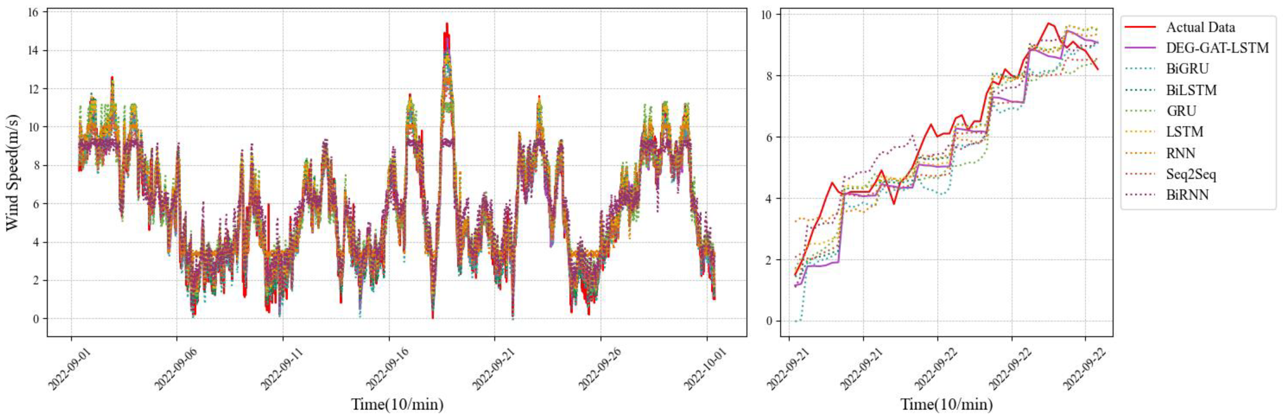
3.3. Experimental Results
3.3.1. Experiment I
- LSTM is a recurrent neural network designed to process sequential data and capture long-term dependencies through gating units.
- BILSTM considers context information simultaneously through forward and backward LSTM layers and is suitable for a variety of sequence tasks.
- GRU is a recurrent neural network similar to LSTM with fewer parameters and a lower computational cost.
- RNN is one of the earliest sequence models, but it faces the vanishing gradient problem and is not suitable for long-term dependence tasks.
- BIRNN combines a forward and backward RNN or LSTM layers to fully understand sequence data and is suitable for a variety of tasks.
- Seq2Seq models are used for sequence-to-sequence tasks, including machine translation and speech recognition, and consist of an encoder and a decoder.
3.3.2. Experiment II
- Model1 purpose: The original model serves as a baseline for comparison
- Model without residuals: model2 Objective: To analyze the effect of the residual structure
- Model without graph attention: model3 Objective: To verify the effectiveness of the graph attention mechanism
- Model without LSTM: model4 Objective: To test the effect of LSTM on the model performance
- Model5 without DGE objective: To test the performance of dynamic graph embedding
4. Conclusions and Future Work
Author Contributions
Funding
Institutional Review Board Statement
Informed Consent Statement
Data Availability Statement
Conflicts of Interest
Nomenclature
| NWP | Numerical weather prediction |
| ML | Machine learning |
| BP | Back propagation |
| MLP | Multilayer perceptrons |
| CNN | Convolutional neural network |
| PDCNN | Predictive depth convolutional neural network |
| GRU | Gated recurrent units |
| GCN | Graph convolutional network |
| LSTM | Long short term memory |
| RNN | Recurrent neural network |
| EMD | Empirical mode decomposition |
| GAT | Graph attention network |
| GNN | Graph neural network |
| SHM | Health monitoring system |
| RMSE | Root mean squared error |
| MAE | Mean absolute error |
| MSE | Mean squared error |
| DTW | Dynamic time warping |
| DGE | Dynamic graph embedding |
| NDBC | National buoy data center |
| ANN | Artificial neural network |
References
- Suo, L.; Peng, T.; Song, S.; Zhang, C.; Wang, Y.; Fu, Y.; Nazir, M.S. Wind speed prediction by a swarm intelligence based deep learning model via signal decomposition and parameter optimization using improved chimp optimization algorithm. Energy 2023, 276, 127526. [Google Scholar] [CrossRef]
- Khosravi, A.; Machado, L.; Nunes, R.O. Time-series prediction of wind speed using machine learning algorithms: A case study Osorio wind farm, Brazil. Appl. Energy 2018, 224, 550–566. [Google Scholar] [CrossRef]
- Liu, X.; Lin, Z.; Feng, Z. Short-term offshore wind speed forecast by seasonal ARIMA—A comparison against GRU and LSTM. Energy 2021, 227, 120492. [Google Scholar] [CrossRef]
- Peng, X.; Wang, H.; Lang, J.; Li, W.; Xu, Q.; Zhang, Z.; Cai, T.; Duan, S.; Liu, F.; Li, C. EALSTM-QR: Interval wind-power prediction model based on numerical weather prediction and deep learning. Energy 2021, 220, 119692. [Google Scholar] [CrossRef]
- Rodrigues, S.; Restrepo, C.; Kontos, E.; Pinto, R.T.; Bauer, P. Trends of offshore wind projects. Renew. Sustain. Energy Rev. 2015, 49, 1114–1135. [Google Scholar] [CrossRef]
- Gao, Z.; Li, Z.; Xu, L.; Yu, J. Dynamic adaptive spatio-temporal graph neural network for multi-node offshore wind speed forecasting. Appl. Soft Comput. 2023, 141, 110294. [Google Scholar] [CrossRef]
- Geng, X.; Xu, L.; He, X.; Yu, J. Graph optimization neural network with spatio-temporal correlation learning for multi-node offshore wind speed forecasting. Renew. Energy 2021, 180, 1014–1025. [Google Scholar] [CrossRef]
- Ren, Y.; Li, Z.; Xu, L.; Yu, J. The data-based adaptive graph learning network for analysis and prediction of offshore wind speed. Energy 2023, 267, 126590. [Google Scholar] [CrossRef]
- Xu, L.; Ou, Y.; Cai, J.; Wang, J.; Fu, Y.; Bian, X. Offshore wind speed assessment with statistical and attention-based neural network methods based on STL decomposition. Renew. Energy 2023, 216, 119097. [Google Scholar] [CrossRef]
- Sun, W.; Gao, Q. Short-Term Wind Speed Prediction Based on Variational Mode Decomposition and Linear–Nonlinear Combination Optimization Model. Energies 2019, 12, 2322. [Google Scholar] [CrossRef]
- Yang, M.; Guo, Y.; Huang, Y. Wind power ultra-short-term prediction method based on NWP wind speed correction and double clustering division of transitional weather process. Energy 2023, 282, 128947. [Google Scholar] [CrossRef]
- Tian, Z.; Li, H.; Li, F. A combination forecasting model of wind speed based on decomposition. Energy Rep. 2021, 7, 1217–1233. [Google Scholar] [CrossRef]
- Qu, Z.; Li, J.; Hou, X.; Gui, J. A D-stacking dual-fusion, spatio-temporal graph deep neural network based on a multi-integrated overlay for short-term wind-farm cluster power multi-step prediction. Energy 2023, 281, 128289. [Google Scholar] [CrossRef]
- Zhang, Y.; Pan, G.; Chen, B.; Han, J.; Zhao, Y.; Zhang, C. Short-term wind speed prediction model based on GA-ANN improved by VMD. Renew. Energy 2020, 156, 1373–1388. [Google Scholar] [CrossRef]
- Zhang, D.; Lou, S. The application research of neural network and BP algorithm in stock price pattern classification and prediction. Future Gener. Comput. Syst. 2021, 115, 872–879. [Google Scholar] [CrossRef]
- Khan, Z.Y.; Niu, Z. CNN with depthwise separable convolutions and combined kernels for rating prediction. Expert Syst. Appl. 2021, 170, 114528. [Google Scholar] [CrossRef]
- Wang, J.; Li, X.; Li, J.; Sun, Q.; Wang, H. NGCU: A New RNN Model for Time-Series Data Prediction. Big Data Res. 2022, 27, 100296. [Google Scholar] [CrossRef]
- Zhang, D.; Kabuka, M.R. Combining weather condition data to predict traffic flow: A GRU-based deep learning approach. IET Intell. Transp. Syst. 2018, 12, 578–585. [Google Scholar] [CrossRef]
- Liu, X.; Zhang, H.; Kong, X.; Lee, K.Y. Wind speed forecasting using deep neural network with feature selection. Neurocomputing 2020, 397, 393–403. [Google Scholar] [CrossRef]
- Ding, Y.; Ye, X.-W.; Guo, Y. A Multistep Direct and Indirect Strategy for Predicting Wind Direction Based on the EMD-LSTM Model. Struct. Control Health Monit. 2023, 2023, 4950487. [Google Scholar] [CrossRef]
- Karim, F.K.; Khafaga, D.S.; Eid, M.M.; Towfek, S.K.; Alkahtani, H.K. A Novel Bio-Inspired Optimization Algorithm Design for Wind Power Engineering Applications Time-Series Forecasting. Biomimetics 2023, 8, 321. [Google Scholar] [CrossRef]
- Huang, Y.; Zhang, B.; Pang, H.; Wang, B.; Lee, K.Y.; Xie, J.; Jin, Y. Spatio-temporal wind speed prediction based on Clayton Copula function with deep learning fusion. Renew. Energy 2022, 192, 526–536. [Google Scholar] [CrossRef]
- Zhu, Q.; Chen, J.; Zhu, L.; Duan, X.; Liu, Y. Wind Speed Prediction with Spatio–Temporal Correlation: A Deep Learning Approach. Energies 2018, 11, 705. [Google Scholar] [CrossRef]
- Xiong, B.; Lou, L.; Meng, X.; Wang, X.; Ma, H.; Wang, Z. Short-term wind power forecasting based on Attention Mechanism and Deep Learning. Electr. Power Syst. Res. 2022, 206, 107776. [Google Scholar] [CrossRef]
- Dong, D.; Wang, S.; Guo, Q.; Li, X.; Zou, W.; You, Z. Ocean Wind Speed Prediction Based on the Fusion of Spatial Clustering and an Improved Residual Graph Attention Network. J. Mar. Sci. Eng. 2023, 11, 2350. [Google Scholar] [CrossRef]
- Liu, J.; Yang, X.; Zhang, D.; Xu, P.; Li, Z.; Hu, F. Adaptive Graph-Learning Convolutional Network for Multi-Node Offshore Wind Speed Forecasting. J. Mar. Sci. Eng. 2023, 11, 879. [Google Scholar] [CrossRef]
- Khodayar, M.; Wang, J. Spatio-Temporal Graph Deep Neural Network for Short-Term Wind Speed Forecasting. IEEE Trans. Sustain. Energy 2019, 10, 670–681. [Google Scholar] [CrossRef]
- Yu, M.; Zhang, Z.; Li, X.; Yu, J.; Gao, J.; Liu, Z.; You, B.; Zheng, X.; Yu, R. Superposition Graph Neural Network for offshore wind power prediction. Future Gener. Comput. Syst. 2020, 113, 145–157. [Google Scholar] [CrossRef]
- Xu, X.; Hu, S.; Shao, H.; Shi, P.; Li, R.; Li, D. A spatio-temporal forecasting model using optimally weighted graph convolutional network and gated recurrent unit for wind speed of different sites distributed in an offshore wind farm. Energy 2023, 284, 128565. [Google Scholar] [CrossRef]
- National Buoy Data Center. Available online: https://www.ndbc.noaa.gov/historical_data.shtml (accessed on 23 December 2023).
- Riley, R. NDBC Wave observation system update. Coast. Eng. J. 2023, 1–7. [Google Scholar] [CrossRef]
- Yang, T.; Hu, L.; Shi, C.; Ji, H.; Li, X.; Nie, L. HGAT: Heterogeneous graph attention networks for semi-supervised short text classification. ACM Trans. Inf. Syst. 2021, 39, 1–29. [Google Scholar] [CrossRef]


| Number of Buoy | Size | Max (m/s) | Min (m/s) | Mean (m/s) | Std (m/s) | Skewness | Kurtosis |
|---|---|---|---|---|---|---|---|
| 46002 | 43,751 | 16.7 | 0.0 | 6.38 | 2.87 | 0.31 | −0.13 |
| 46011 | 43,751 | 16.3 | 0.0 | 6.22 | 3.07 | 0.11 | −0.84 |
| 46014 | 43,751 | 17.8 | 0.0 | 5.88 | 3.56 | 0.53 | −0.52 |
| 46025 | 43,751 | 16.2 | 0.0 | 3.44 | 2.15 | 1.39 | 3.03 |
| 46028 | 43,751 | 17.6 | 0.0 | 7.18 | 3.86 | 0.03 | −1.11 |
| 46042 | 43,751 | 15.7 | 0.0 | 6.19 | 3.16 | 0.16 | −0.8 |
| 46059 | 43,751 | 14.2 | 0.0 | 6.09 | 2.58 | 0.19 | −0.53 |
| 46072 | 43,751 | 20.9 | 0.0 | 5.92 | 3.66 | 0.41 | −0.62 |
| 46084 | 43,751 | 21.0 | 0.0 | 6.68 | 3.66 | 0.58 | −0.19 |
| 46089 | 43,751 | 19.6 | 0.0 | 6.05 | 2.94 | 0.3 | −0.25 |
| 51000 | 43,751 | 12.6 | 0.0 | 6.13 | 2.10 | −0.31 | −0.44 |
| 51004 | 43,751 | 15.7 | 0.0 | 7.23 | 1.80 | −0.41 | 0.79 |
| Model | Specific Description |
|---|---|
| LSTM | The internal parameters were randomized, 1 LSTM layer, 128 hidden dimensions, and a linear layer. |
| BILSTM | The internal parameters were randomized, 1 bidirectional LSTM layer, 128 hidden dimensions, and a linear layer. |
| GRU | The internal parameters were randomized, 3 GRU layers, 128 hidden dimensions, and one linear layer. |
| BIGRU | The internal parameters were randomized, 3 bidirectional GRU layers, 128 hidden dimensions, and one linear layer. |
| RNN | The internal parameters were randomized, 1 RNN layer, 128 hidden dimensions, and a linear layer. |
| BIRNN | The internal parameters were randomized, 1 bidirectional RNN layer, 128 hidden dimensions, and a linear layer. |
| Seq2Seq | The internal parameters were randomized, LSTM is used as encoder, 2 LSTM layers with 64 hidden dimensions and MLP is used as decoder. |
| DGE-GAT-LSTM | 2 layers of GAT network with 4 attention heads, one layer of LSTM, GAT network and LSTM are serially connected. 2 linear layers with nonlinear activation. |
| Model | MAE (m/s) | RMSE (m/s) | ||||
|---|---|---|---|---|---|---|
| 1-Step (10 min) | 6-Step (1 h) | 24-Step (4 h) | 1-Step (10 min) | 6-Step(1 h) | 24-Step (4 h) | |
| LSTM | 0.3425 | 0.5946 | 0.9801 | 0.4620 | 0.7750 | 1.2968 |
| BILSTM | 0.3447 | 0.5903 | 0.9493 | 0.4648 | 0.7740 | 1.2651 |
| GRU | 0.3561 | 0.7306 | 0.9448 | 0.4734 | 0.9412 | 1.2694 |
| BIGRU | 0.3570 | 0.5780 | 0.9602 | 0.4769 | 0.7633 | 1.2916 |
| RNN | 0.3604 | 0.7635 | 0.9789 | 0.4903 | 1.0036 | 1.3009 |
| BIRNN | 0.3650 | 0.7304 | 0.9527 | 0.4967 | 0.9598 | 1.2851 |
| Seq2Seq | 0.3450 | 0.5995 | 1.0059 | 0.4623 | 0.7837 | 1.3250 |
| DGE-GAT-LSTM | 0.3396 | 0.5571 | 0.9333 | 0.4546 | 0.7363 | 1.2501 |
| Model | MAE (m/s) | Percentage | RMSE (m/s) | Percentage |
|---|---|---|---|---|
| 1-Step (10 min) | 1-Step (10 min) | |||
| Model1 | 0.3419 | 0% | 0.4549 | 0% |
| Model2 | 0.4298 | +25.69% | 0.5548 | +21.96% |
| Model3 | 0.3729 | +9.06% | 0.5027 | +10.50% |
| Model4 | 1.9339 | +465.57% | 2.3262 | +411.37% |
| Model5 | 0.4112 | +20.26% | 0.5361 | +17.84% |
Disclaimer/Publisher’s Note: The statements, opinions and data contained in all publications are solely those of the individual author(s) and contributor(s) and not of MDPI and/or the editor(s). MDPI and/or the editor(s) disclaim responsibility for any injury to people or property resulting from any ideas, methods, instructions or products referred to in the content. |
© 2024 by the authors. Licensee MDPI, Basel, Switzerland. This article is an open access article distributed under the terms and conditions of the Creative Commons Attribution (CC BY) license (https://creativecommons.org/licenses/by/4.0/).
Share and Cite
Dong, D.; Wang, S.; Guo, Q.; Ding, Y.; Li, X.; You, Z. Short-Term Marine Wind Speed Forecasting Based on Dynamic Graph Embedding and Spatiotemporal Information. J. Mar. Sci. Eng. 2024, 12, 502. https://doi.org/10.3390/jmse12030502
Dong D, Wang S, Guo Q, Ding Y, Li X, You Z. Short-Term Marine Wind Speed Forecasting Based on Dynamic Graph Embedding and Spatiotemporal Information. Journal of Marine Science and Engineering. 2024; 12(3):502. https://doi.org/10.3390/jmse12030502
Chicago/Turabian StyleDong, Dibo, Shangwei Wang, Qiaoying Guo, Yiting Ding, Xing Li, and Zicheng You. 2024. "Short-Term Marine Wind Speed Forecasting Based on Dynamic Graph Embedding and Spatiotemporal Information" Journal of Marine Science and Engineering 12, no. 3: 502. https://doi.org/10.3390/jmse12030502
APA StyleDong, D., Wang, S., Guo, Q., Ding, Y., Li, X., & You, Z. (2024). Short-Term Marine Wind Speed Forecasting Based on Dynamic Graph Embedding and Spatiotemporal Information. Journal of Marine Science and Engineering, 12(3), 502. https://doi.org/10.3390/jmse12030502