Abstract
Time series prediction is an effective tool for marine scientific research. The Hierarchical Temporal Memory (HTM) model has advantages over traditional recurrent neural network (RNN)-based models due to its online learning and prediction capabilities. Given that the neuronal structure of HTM is ill-equipped for the complexity of long-term marine time series applications, this study proposes a new, improved HTM model, incorporating Gated Recurrent Units (GRUs) neurons into the temporal memory algorithm to overcome this limitation. The capacities and advantages of the proposed model were tested and evaluated on time series data collected from the Xiaoqushan Seafloor Observatory in the East China Sea. The improved HTM model both outperforms the original one in short-term and long-term predictions and presents results with lower errors and better model stability than the GRU model, which is proficient in long-term predictions. The findings allow for the conclusion that the mechanism of online learning has certain advantages in predicting ocean observation data.
1. Introduction
Time series prediction focuses on identifying patterns in historical sequence data and providing new data prediction, which plays an important role in various disciplines including sociology [], finance [], transportation [], industry [,], and marine science [,]. With advancements in ocean observation technologies, a diverse range of data reflecting the characteristics of marine space–time processes has been continuously collected. However, the intricacies of the marine environment pose challenges for characterizing the space–time processes of the ocean merely with raw observation data. Accurate time series prediction is thus crucial for monitoring the marine environment, comprehending the evolution of marine space–time processes, predicting marine climate phenomena, and fostering sustainable marine development.
Long-term and high-temporal-resolution oceanographic data are of paramount importance for scientific discoveries in oceanography research. However, the limitations of sensors and transmission technologies have incommodated continuous and long-term ocean time series data acquisition in recent decades. Recent advances in copper-fiber undersea cables, wet-mated connections, autonomous sensors, and communications have enabled networked and cabled ocean observations. This enables a large volume of continuous and high-temporal-resolution observation data acquisition, allowing for a better understanding of the evolution of marine spatial–temporal processes and significant improvements in the capability, accuracy, and efficiency of prediction of ocean phenomena. These observation data give researchers an opportunity to utilize various time series forecasting methods to predict observational parameters for both the ocean surface and the deep sea [,,,,], for the purpose of enhancing insights into oceanic environmental conditions, marine spatial–temporal process evolution, and marine phenomena and disasters.
The approaches of time series data analysis can be catalogued as statistics, machine learning, and deep learning. Traditional statistics-based approaches such as the autoregressive integrated moving average (ARIMA) model and wavelet analysis [] have been widely employed in various fields such as finance analysis [], traffic flow predictions [], and chlorophyll concentration estimations [,]. ARIMA is typically suitable for stationary time series because it incorporate autoregression, differencing, and moving average components []. To address cyclical and seasonal patterns, the seasonal ARIMA (SARIMA) model has been further developed as an extension of ARIMA, and offers an improved forecasting performance considering seasonal factors. However, these methods commonly present poor abilities to capture nonlinear relationships within time series data, and thus fail to provide reliable predictions for complex oceanic observation data [].
Due to their remarkable nonlinear fitting abilities, machine learning algorithms and deep learning models have been widely adopted for performing time series prediction among the oceanographic community in recent years. Traditional machine learning algorithms such as support vector machines (SVMs) and random forest (RF) algorithms have exhibited decent performances in areas like traffic flow and wave height prediction [,]. However, their effectiveness in handling complex sequences and long-term forecasting is slightly inadequate; thus, it is difficult to achieve satisfactory prediction results based on ocean time series data [,]. To address these limitations and challenges, deep learning approaches have been developed to model and predict time series data. Deep learning models have outstanding feature learning and nonlinear fitting abilities, and present numerous advantages over traditional machine learning algorithms for time series prediction.
The recurrent neural network (RNN) is a type of neural network model representatively designed for processing time series data. RNN has a recurrent structure that facilitates the effective capture and remembering of the contextual relationships within time series data. Therefore, RNNs have been widely employed to perform data analysis such as time series prediction and natural language processing. However, conventional RNNs are inherently limited in long-term sequence predictions due to the error backpropagation usage in weight updates, resulting in problems of vanishing or exploding gradients. In 1997, Hochreiter and Schmidhuber proposed long short-term memory (LSTM) with a unique structure known as the gate mechanism [] to address these challenges. The gate mechanism allows LSTM neurons to selectively “forget” certain unimportant information during the learning process, which effectively solves the problems of gradient vanishing and explosion and presents better long-term memory capabilities.
Regarding the existing deep learning models, RNN and its variants such as LSTM and gate recurrent units (GRUs) [] have demonstrated high efficiency and superb prediction accuracy in long-term complex time series forecasting. They have been successfully adopted to predict sea surface temperature, sea-level height, sea ice, dissolved oxygen, chlorophyll, and pore water characteristics [,,,,,,]. Moreover, the high scalability advantage enables these algorithms to effectively handle diverse types of complex and long-term time series data by either adjusting their scales and internal structures or integrating them with other methods [,,,,].
Although RNNs enable effective complex nonlinear time series data analysis, their prediction accuracy depends on excellent network structure design, appropriate activation and loss functions, reasonable training strategies, and precise parameter tuning. In particular, it is necessary to adjust the model’s structures and parameters to accommodate changes in data types, attribute dimensions, sampling frequency, and other relevant factors. The uncertainty and randomness inherent in marine environment observation data additionally pose significant challenges in ocean time series prediction, which could cause the models’ accuracy to gradually decrease over time due to their lack of online learning capabilities. To resolve this issue, updating the model periodically with new transmitted sensor data [] or utilizing networks with online learning capabilities [] could offer alternative solutions. As a representative method with online learning and prediction capabilities, HTM (Hierarchical Temporal Memory) has been increasingly adopted for time series prediction in recent years.
HTM is a deep learning technology [] that aims to mimic the structure and algorithmic characteristics of the neocortex. It converts complex problems into pattern matching and prediction by extracting spatial and temporal features from data and using Sparse Distributed Representation (SDR) to tackle online analysis and the prediction of data streams. One notable advantage of HTM is its ability to handle multiple tasks with one single set of parameters, which effectively reduces the complexity of network building and parameter tuning. Its efficient and flexible capabilities of online learning and prediction have been demonstrated in various applications including short-term traffic flow forecasting [], anomaly detection [], and Numenta Anomaly Benchmark (NAB) dataset [] in comparison with ARIMA, LSTM, and other methods. Moreover, HTM also shows promising performance in the object recognition and classification of moving objects and trajectory sequences [,,].
However, previous investigations into HTM improvements have primarily focused on enhancing its structure design and combining it with other neural network models [,,]; few studies have addressed its ineffectiveness in detecting and capturing correlated information from longer time series, particularly in the field of oceanography. In this study, we developed an improved HTM model by integrating GRU neurons into the HTM network. The GRU-based approach significantly enhances the long-term prediction performance of the model while preserving the original online learning and prediction capabilities. The effectiveness of the proposed model has been validated in experiments using a time series observational dataset, including temperature, pressure, and conductivity, collected from the Xiaoqushan Seafloor Observatory in the East China Sea.
The content of this paper is organized into the following sections: An overview of the time series prediction algorithms and their related works is presented in Section 1. Section 2 describes the principles of GRU, HTM, and the improvement method in detail. Section 3 presents our experiments and a discussion of the improved HTM model. Section 4 summarizes the main conclusions of this study.
2. Methodology
2.1. Gated Recurrent Units (GRUs)
GRUs are considered to be further simplifications of the LSTM model. In GRU, conventional components of LSTM, including input gate, forget gate, and output gate, are replaced by the reset gate and the update gate []. This simplification leads to a lower number of parameters and computational requirements in comparison with LSTM. Moreover, GRU demonstrates comparable learning capabilities and predictive accuracy, while being more computationally efficient and easier to train in various tasks than LSTM is. These advantages have led to GRUs being rapidly adopted by researchers in the field of time series prediction.
The detailed structure of GRU is shown in Figure 1, where represents the inputs data at time stept, and represents the hidden state propagated from the previous neuron during the training process. Firstly, the current neuron calculates the state of the reset gate (Equation (1)) and the update gate (Equation (2)) based on these two inputs.
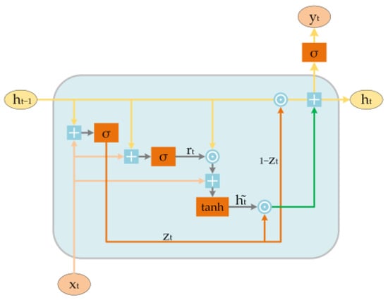
Figure 1.
The structure of gate recurrent unit (GRU) neuron. ⊙ represents Hadamard product.
The reset gate () allows the network to selectively discard previous information. The model will forget the calculated state and relearn from the input (Equation (3)) if is 0, which means that the reset gate is closed.
The update gate () is utilized to retain information from previous time steps (Equation (4)).
Lastly, the output is computed based on the state of the neuron at time step , denoted as (Equation (5)).
The weight matrices , , and correspond to the inputs, while is associated with the output. The , , and represent the weight matrices related to the hidden state of the GRU neurons. Their dimensions are associated with the structure of the HTM model and will be elucidated in the Algorithm and Model Implementation Sections. is the sigmoid activation function and represents the Hadamard product.
2.2. Hierarchical Temporal Memory (HTM)
HTM (Hierarchical Temporal Memory) is an unsupervised learning algorithm which incorporates a wealth of scientific knowledge about the neural system and borrows many terms from neuroscience. Figure 2a illustrates a biological neuron cell; similarly, Figure 2b shows a simplified HTM cell model. In this model, proximal dendrites (green) are responsible for receiving the feed-forward inputs that are shared among the internal cells of the columns, while the distal dendrites (blue) receive the inputs from the other cells within the same hierarchy. Each cell contains multiple distal dendrites, and these dendrites form multiple synapses (dots) with other cells. The synapses in HTM have dynamically changing “permanence values” that represent the stability of the connections and will be activated when the scalar “permanence value” surpasses the predefined threshold.
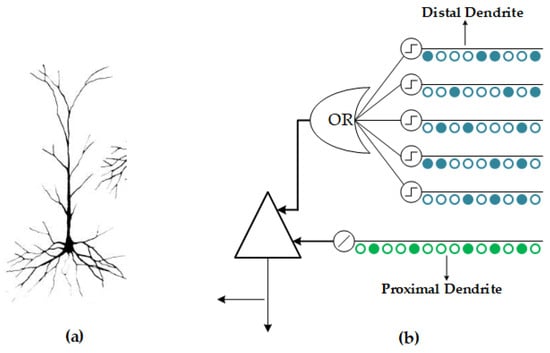
Figure 2.
(a) Biological neuron; (b) Hierarchical Temporal Memory (HTM) cell.
HTM is characterized by a prominent hierarchy that differs from those of RNNs. In HTM, multiple foundational pattern sequences stored at lower levels are aggregated to form more complex pattern sequences as the hierarchy ascends. Additionally, HTM cells within the same hierarchy can establish connections and share information with each other, which endows the HTM with a robust generalization capability and a capacity to handle multiple tasks with identical parameters.
In HTM, the prediction process involves several steps: encoding, spatial pooling, temporal memory, and the generation of results through the CLA classifier, as shown in Figure 3. The blue rectangle and arrow in Figure 3 signify the prediction process of the original HTM, whereas the orange rectangle and arrow represent the prediction process of the improved HTM.

Figure 3.
The prediction process of original and improved HTM.
- Sparse Distributed Representation Encoders: Unlike GRUs, HTM completes the entire prediction process through state transitions of cells, with the inactive state represented by a value of 0; meanwhile, the predictive and active states correspond to a value of 1. Consequently, prior to spatial pooling, the input data need to be encoded into 0–1 sequences using various encoders, such as the temporal encoder and the scalar encoder. These encoders are employed to handle the temporal and numerical information separately. Output sequences of encoders are referred to as Sparse Distributed Representation (SDR) sequences, which possess a sparsity characteristic. In fixed-length sequences, the proportion of “1” typically ranges from 0.02 to 0.04. Additionally, SDR sequences can be combined and decomposed through binary operations, such as “AND”, “OR”, and “NOT”. This allows for the efficient utilization of storage space and ensures stable computation speed, regardless of network scale.
- Spatial Pooler: Multiple “cell columns” composed of cells are vertically arranged to create a “region” horizontally. Each column corresponds to a specific binary sequence and becomes active when that particular sequence appears in the input sequence. The activity level in a cell column is determined by multiplying the number of active synapses in each active cell column by a corresponding “boost factor”. This boost factor is dynamically adjusted based on the activation frequency relative to the surrounding columns. The most active column inhibits a fixed proportion of other columns within the inhibition radius. This mechanism ensures that the spatial pooler maintains sparsity. Each input bit (0 or 1) corresponds to a cell within the active column, resulting in an increase or a decrease in the permanence value of synapses. Furthermore, the input activity level of cell columns that have never been activated will be enhanced until they become active to ensure that all columns contribute to the prediction results.
- Temporal Memory: In HTM, cells are activated in correspondence to each active column. However, if there are no cells in the predictive state, then all cells within the column will be activated. The dendritic segment is considered to be active when the number of active synapses connected to active cells surpasses a predefined threshold. When an HTM cell possesses an active dendritic segment, it will transition into the predictive state. The combination of cells in both the active and predictive states contribute to generating the prediction result also known as SDR for the specific region at the current time.
The permanence values of synapses undergo an increase and a decrease when they are connected to active cells and inactive cells, respectively. Furthermore, the dendritic segments that best match the previous prediction patterns are repeatedly selected and undergo the aforementioned operations to enhance their long-term prediction performance. However, these modifications only take effect upon the arrival of the next input corresponding to the column; otherwise, they remain invalid. Only cells activated in the predictive state at the current moment are considered to be correct predictions; this represents the “reward” and “punishment” mechanisms of the HTM. The increase and decrease in the synaptic permanence values induce changes in the states of some synapses; thus, the states of the dendritic segments and the cells are converted, and the predictions in the subsequent moment are ultimately influenced.
- 4.
- CLA Classifier: The internal structure of the CLA classifier is a single-layer feed-forward neural network. The input layer neurons correspond to the SDR sequence generated by TM, and the size of output layer depends on the parameters set up by the encoders. Essentially, the CLA classifier serves as a decoder by establishing one-to-one mapping between the output layer and the data.
It is evident that the HTM accomplishes “learning” and “prediction” through the distinct steps of spatial pooling and temporal memory. The online learning capability of HTM can be controlled by enabling or disabling the modification of synaptic values during the spatial pooling step.
2.3. GRU-Based HTM Improvement
The predictions of HTM are produced by cells transitioning into the predictive state from the previous time step. However, the inherent function of HTM cells is primarily to store the permanence values of synapses and these cells do not possess intrinsic memory capabilities. Consequently, it poses challenges for achieving a satisfactory prediction performance in the complex time series characterized by long durations and substantial temporal dependencies. In this study, we integrated the GRU neuron into the HTM network for the purpose of enhancing the ability of capturing complex event information and improving the accuracy of model calculations in long-term prediction.
Considering the advantages of GRU units, we propose the improved HTM algorithm based on the GRU model. In the improved HTM model, the input vector of GRU is constructed by taking into account the number of effective synapses in each dendritic segment of HTM cells. In contrast to the original temporal memory algorithm, the cell state is considered to be active and is set to 1 when the GRU computation result exceeds a predefined threshold. Meanwhile, the previous rule of converting the cell state based on the presence of active dendritic segments in cells is discarded. The final prediction outcome is obtained through the CLA classifier, where an SDR generated from temporal memory is input following these computations. The detailed process of improved HTM prediction is illustrated in Figure 3.
2.3.1. Weight Update Algorithm of GRU
The computation process of GRU prediction is elaborated in Section 2.1. During this process, the weight matrices , , , , , , and are initialized with random values, representing the weight matrices of the corresponding parameters. Subsequent to the prediction carried out by GRU, the weight matrices are updated based on the gradients of the prediction error. Detailed calculation steps are outlined in the following.
The square error of prediction is selected as the loss function, where represents the measured value, represents the predicted value, and represents the current time step.
The gradient of the parameter matrix can be calculated and vectorized using Equations (7)–(19):
The notation in the aforementioned equations refers to the parameters corresponding to the subsequent neuron and the apex T indicates the transpose of matrix.
GRU outputs are calculated using the equations described in Section 2.1 and the gradients are computed based on the error. The weight matrices are then updated utilizing Equation (20).
The learning rate, denoted as “learningRate”, is a hyperparameter used to regulate the degree to which a model learns from the current input. It determines the magnitude of the parameter updates during the training process.
2.3.2. Improved Temporal Memory Theory
By integrating GRU neurons into the HTM network, the temporal memory algorithm can be improved and implemented through the following computation process:
- Retrieve the count of active synapses in each dendritic segment of HTM cells at time step using the built-in method provided by HTM. Here, represents the number of dendritic segments per cell.
- 2.
- Calculate the GRU output according to the process described in Section 2.1.
- 3.
- Activate the cells if the output surpasses the predefined threshold.
- 4.
- Compute the square error and update the GRU weight parameters.
The reward and punishment mechanisms are preserved in the improved HTM. However, the original rule of cell activation based on the number of active synapses in dendritic segments has been discarded, as the improved HTM relies solely on the output of GRU. Additionally, the improved HTM introduces two hyperparameters: the learning rate can be initially set and dynamically adjusted using the Adam algorithm, while the activation threshold, denoted as “μ”, requires parameter tuning.
2.4. Algorithm and Model Implementation
The htm.core of the 2.1.16 version is a software implementation of the HTM algorithm, encompassing various components such as the encoder, the spatial pooler, the temporal memory, and the predictor. This comprehensive tool has been adopted for time series analysis, anomaly detection and data prediction. This htm.core is a Python library designed to run on the Windows platform, with the core algorithms implemented in C++ 17. In this study, we integrated the GRU prediction and training algorithms into the temporal memory process of the HTM by modifying the “TemporalMemory.hpp” and “TemporalMemory.cpp” source code files contained in the htm.core, using the C++ matrix operation library called Eigen. Considering that the cell indices of HTM are stored as a one-dimensional vector, the weight matrices corresponding to the inputs of GRU neurons are set to m × n (m is the number of HTM cells, equal to the product of the number of cell columns and the number of cells in each column; n represents the number of dendritic segments per HTM cell). Since each cell has n dendritic segments, the matrices related to the output and hidden state of GRU neurons are of size m × 1. All these matrices are initialized using the “setRandom” function provided by the Eigen library, assigning random values between 0 and 1. The input vector is obtained through methods contained in the “Connections” class of htm.core. The output of the GRU neuron is calculated to determine whether the cell should be activated through a comparison with “μ”. The weight matrices are updated by comparing the real results with previous prediction results when the input for the next time step arrives and activates the cell. Hyperparameters such as “LearningRate” and “μ” have been incorporated into the Python methods, allowing for flexible adjustments in practical applications.
2.5. Performance Metrics
To assess and compare the performance of the improved HTM model, we utilize the mean absolute percentage error () and the root mean square error () as evaluation metrics. The formulas for these metrics are described as follows:
where represents the measured value, represents the predicted value, and represents the total number of samples.
3. Experiments and Discussion
To evaluate the capacity and advantage of the proposed improved HTM model, several experiments were performed in this section. The experiments were conducted on a workstation running Windows Professional Edition (version 21H2). The hardware specifications included an Intel Xeon® W-2295 CPU, 128 GB of RAM, Python version 3.9.18, PyTorch version 2.1.0, and CUDA version 121.
3.1. Data Description
The Xiaoqushan Seafloor Observatory in the East China Sea is located near Xiaoqushan Island at coordinates 30.5° N, 122.2° E (Figure 4). It is approximately 20 km southeast of the Yangshan Deepwater Port and is characterized by an average water depth of 15 m. The station is situated in an irregular semidiurnal shallow tide zone adjacent to the deep-water channel, equipped with a variety of sensors including CTD and ADCP. Continuous observation data of temperature (7.5996 °C to 29.1057 °C), pressure (12.0439 dbar to 17.1256 dbar), and conductivity (12.1201 mmho/cm to 84.9530 mmho/cm), with a sampling interval of 10 s, were obtained from August 2014 to August 2015. And the salinity (7.0896 PSU to 87.7200 PSU) data were calculated using conductivity, temperature, and pressure data.
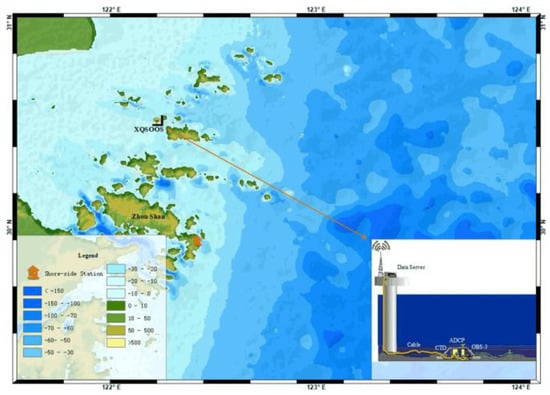
Figure 4.
Xiaoqushan Seafloor Observatory in the East China Sea.
The total experimental data comprise approximately 2.65 million records. About 260,000 records from 15 August to 15 September 2014 were allocated for the model pretraining and parameters tuning steps; meanwhile, testing was conducted using data spanning the entire year (2.65 million records). The training set size for all experiments remained consistent at 10,000 records.
3.2. Model Pretraining
In order to investigate the influence of pretraining on the accuracy of HTM, we calculated the squared errors in a step-by-step manner, as shown in Figure 5. It can be noted that the HTM is unable to generate reasonable predictions, resulting in a considerable error at the initial phase of learning. Nevertheless, as HTM continues to learn, the error decreases significantly and is maintained at a stable level. The mean square errors of the original and improved HTM were 1.69 and 1.39, respectively.
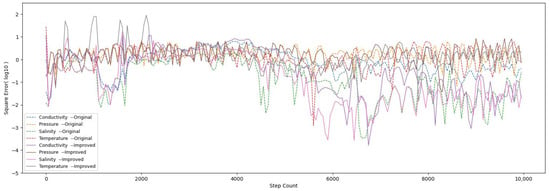
Figure 5.
Step-by-step square error (log10).
To assess the model’s accuracy, we calculated the RMSE of the prediction results on the test set with 1000 time steps for varying numbers of pretraining iterations. The resulting curves are illustrated in Figure 6.

Figure 6.
RMSE with variant training iterations of HTM and improved HTM.
The initial stage of the spatial pooler exhibits an unstable correspondence between the inputs (encoded time series data) and columns, resulting in unsatisfactory model prediction performance. However, a few iterations of pretraining lead to a conspicuous improvement in the model accuracy. It can be consequently inferred that conducting a certain number of pretraining iterations is effective in reducing errors during the initial stage and in expediting the model’s fitting process, though with online learning capabilities.
The prediction error of the original HTM decreased initially but later exhibited an upward trend for the temperature and pressure data, achieving their minimum values at iteration 1; meanwhile, the conductivity and salinity curves repeated at iteration 0, with marginal variance from iteration 1. Considering the HTM’s capability for online learning, the pretraining iterations of the original HTM model were set to 1. Compared to the original version, the improved HTM model maintained a consistent level of accuracy and model stability for iterations exceeding 2. Consequently, the pretraining iterations for the improved HTM model were set to 2.
3.3. Parameters Tuning
To determine the appropriate value for the newly introduced “μ”, specific tuning work was necessary. Meanwhile, the remaining configuration can be directly referenced from the parameters used in the Hotgym prediction example, considering the inherent characteristics of the HTM.
On the one hand, the weight matrices of GRU are initialized using the “setRandom” function from Eigen, which assigns random values between 0 and 1. On the other hand, the number of active synapses in the dendritic segments of the HTM are always greater than or equal to the value of zero. Combining these factors with the properties of the “sigmoid” and “tanh” functions, it can be inferred that the output of the GRU will always fall within the range of 0.5 to 1, setting the values for “μ” accordingly. The prediction errors on temperature, pressure, conductivity, and salinity data at 5 and 1000 time steps are calculated under different values of “μ” and presented in Figure 7.
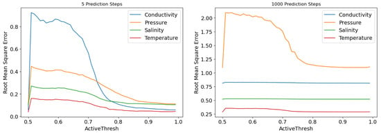
Figure 7.
RMSE with variant activation threshold on various data.
We noted that the error initially rises rapidly and then gradually decreases as the “μ” increases. Another noteworthy aspect is the significant reduction in the time required for single-step prediction as the “μ” increases, accompanied by descending computational complexity resulting from fewer cells being activated. Therefore, the “μ” is determined as 0.99 to strike a balance of accuracy between short-term and long-term predictions.
The model parameters of the HTM are shown in Table 1.

Table 1.
HTM model parameters.
3.4. Performance Evaluation of Improved HTM
3.4.1. Comparison with Original HTM
The prediction results of 1000 time steps are presented in Figure 8. Due to the large number of data points, the actual plotting was performed using a sampling interval for analysis. The measured data are represented by hollow circles in the plot; among these, the predictions made by HTM are indicated by green lines, while the predictions generated by the improved HTM are indicated by red lines.
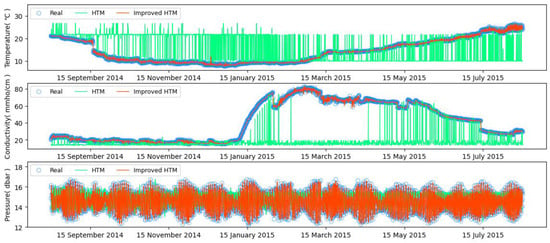
Figure 8.
HTM and improved HTM predictions on temperature and conductivity and pressure data.
The prediction results clearly illustrate that the original HTM is unserviceable, considering the numerous outliers in the form of spikes. In contrast, the improved HTM model with incorporated GRU neurons demonstrates a better fit to the actual values, with fewer outliers. The conductivity prediction results of the original HTM model initially align well with the actual values for the initial several months; meanwhile, significant errors arise later, indicating that the original HTM model is inadequate in capturing information for complex time series with long-term correlations.
To further assess the enhanced capability of the improved HTM model in capturing complex long-term dependencies in time series data, we additionally added a persistence model to the error estimation. It uses the actual values at time to predict the values at time , and the RMSE is calculated for the three models using temperature and conductivity data. The calculations are conducted for time steps of 5, 50, 500, and 1000 with the results presented in the form of boxplots in Figure 9. It is evident that the improved HTM consistently demonstrates smaller maximum error, average error, and median error compared to the persistence model and original HTM. These findings indicate a significant enhancement in the stability and the short- and long-term predictive performances of the improved HTM model in time series data compared to the original HTM.

Figure 9.
RMSE of Persistence Model & HTM & Improved HTM on temperature and conductivity data.
Despite the adoption of C++ to enhance computational efficiency, the improved HTM model requires more time to complete the same number of iterations with a training set containing 10,000 data points (as shown in Figure 10). The increase in training time varies from 22% to 105%, depending on the characteristics of the data and the number of iterations.
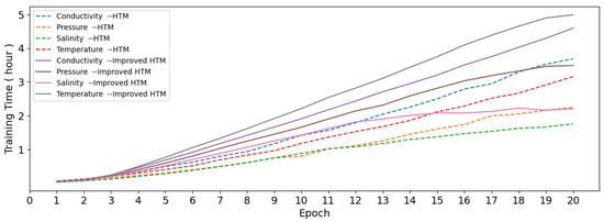
Figure 10.
Training time with variant training iterations of HTM and improved HTM.
3.4.2. Comparison with GRU
The same temperature data used in experiment 1 were chosen for training and testing the GRU model implemented with PyTorch. The prediction was performed using a time step of 1000 with observation window width of 50, while employing the Adam optimizer. By comparing the prediction results of the GRU and improved HTM models in Figure 11, it is obvious that the prediction curve of the GRU closely aligns with that of the improved HTM at the initial stage for months, suggesting comparable performance.
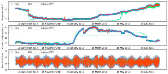
Figure 11.
GRU and improved HTM predictions on temperature, conductivity, and pressure data.
However, the improved HTM consistently outperforms GRU comparing the change in prediction over time. It is worth noting that the error of GRU-based prediction demonstrates a significant increase, while the improved HTM maintains a consistently low level, underscoring the superior performance of online learning method over the traditional offline learning method for ocean time series prediction.
The RMSE for GRU was calculated for various prediction time steps using the same dataset from experiment 2, and the results were visualized through boxplots (Figure 12). The performance of GRU is barely satisfactory in the short-term prediction, as indicated by the slightly higher maximum values, medians, and means of errors compared to the improved HTM. In the context of long-term prediction, the accuracy of improved HTM is, however, superior to that of GRU, with a lower quartile and a lower median of errors as the prediction time steps increase. Additionally, the improved HTM shows advantages, with lower fluctuation and greater stability than GRU.

Figure 12.
RMSE of GRU & Improved HTM on temperature and conductivity data.
4. Conclusions
In this study, we propose an improved HTM model that incorporates GRU neurons into the temporal memory algorithm. The performance of this improved HTM model is evaluated using observation data spanning from August 2014 to August 2015, collected at the Xiaoqushan Seafloor Observatory in the East China Sea. The comparison experiments between the improved model and the initial one validated the effectiveness and enhancement of the proposed improvement algorithm. Furthermore, the improved HTM exhibits notable advantages of online learning in predicting ocean observation data over a long period. Although the improved HTM was solely tested using CTD data, the improved HTM can also be applied to forecast other observation sequences with temporal dependencies.
It should be noted that the proposed algorithm introduces more computational complexity than the original one, while presenting an enhanced capability for capturing and learning from long-term complex time series. In the future, the code implementation will be further optimized to better address this issue.
In addition, parameter tuning is necessary in this study due to the incorporation of additional hyperparameters. It is noteworthy that the original HTM model can handle multiple tasks with identical parameters; this representative characteristic arises from the integration of learning and prediction processes within HTM (online learning). Therefore, a feasible choice for future research involves employing a self-learning network to process inputs and generate tailored outputs, followed by utilizing another network for prediction. This strategy could mitigate the impact of data format disparities on model parameters and streamline the parameter tuning process.
Author Contributions
Conceptualization, T.Q., R.Q. and Y.Y.; methodology, T.Q. and Y.Y.; software, T.Q.; validation, T.Q. and R.C.; formal analysis, T.Q.; investigation, Y.Y. and R.Q.; resources, T.Q. and R.C.; data curation, R.C.; writing—original draft preparation, T.Q.; writing—review and editing, T.Q., R.C., R.Q. and Y.Y.; visualization, T.Q., R.Q. and Y.Y.; supervision, T.Q., R.Q. and Y.Y.; project administration, R.Q.; funding acquisition, R.Q. All authors have read and agreed to the published version of the manuscript.
Funding
This research was funded by the Innovation Program of Shanghai Municipal Education Commission, grant number 2021-01-07-00-07-E00093,the National Key Research and Development Program of China, grant number 2021YFC2800501 and the Interdisciplinary Project in Ocean Research of Tongji University, grant number 2022-2-ZD-04.
Institutional Review Board Statement
Not applicable.
Informed Consent Statement
Not applicable.
Data Availability Statement
The data presented in this study are available on request from the corresponding author (accurately indicate status).
Acknowledgments
The authors are grateful to Yang Yu and Rufu Qin for their support in the theoretical aspects of this study. The authors thank Rufu Qin, Yang Yu and Ruixin Chen for their help in reviewing and editing this paper. We also thank the reviewers and editors for their suggestions to improve the quality of this paper.
Conflicts of Interest
The authors declare no conflicts of interest.
References
- Jiao, F.; Huang, L.; Song, R.; Huang, H. An Improved STL-LSTM Model for Daily Bus Passenger Flow Prediction during the COVID-19 Pandemic. Sensors 2021, 21, 5950. [Google Scholar] [CrossRef]
- Wu, C.; Wang, J.; Hao, Y. Deterministic and uncertainty crude oil price forecasting based on outlier detection and modified multi-objective optimization algorithm. Resour. Policy 2022, 77, 102780. [Google Scholar] [CrossRef]
- Zhang, J.; Wang, P.; Yan, R.; Gao, R.X. Long short-term memory for machine remaining life prediction. J. Manuf. Syst. 2018, 48, 78–86. [Google Scholar] [CrossRef]
- Wu, J.; Hu, K.; Cheng, Y.; Zhu, H.; Shao, X.; Wang, Y. Data-driven remaining useful life prediction via multiple sensor signals and deep long short-term memory neural network. ISA Trans. 2020, 97, 241–250. [Google Scholar] [CrossRef]
- Hu, S.; Shao, Q.; Li, W.; Han, G.; Zheng, Q.; Wang, R.; Liu, H. Multivariate Sea Surface Prediction in the Bohai Sea Using a Data-Driven Model. J. Mar. Sci. Eng. 2023, 11, 2096. [Google Scholar] [CrossRef]
- Alenezi, N.; Alsulaili, A.; Alkhalidi, M. Prediction of Sea Level in the Arabian Gulf Using Artificial Neural Networks. J. Mar. Sci. Eng. 2023, 11, 2052. [Google Scholar] [CrossRef]
- Xiao, C.; Chen, N.; Hu, C.; Wang, K.; Gong, J.; Chen, Z. Short and mid-term sea surface temperature prediction using time-series satellite data and LSTM-AdaBoost combination approach. Remote Sens. Environ. 2019, 233, 111358. [Google Scholar] [CrossRef]
- Du, X.; Sun, Y.; Song, Y.; Yu, Y.; Zhou, Q. Neural network models for seabed stability: A deep learning approach to wave-induced pore pressure prediction. Front. Mar. Sci. 2023, 10, 1322534. [Google Scholar] [CrossRef]
- Shamshirband, S.; Jafari Nodoushan, E.; Adolf, J.E.; Abdul Manaf, A.; Mosavi, A.; Chau, K.-W. Ensemble models with uncertainty analysis for multi-day ahead forecasting of chlorophyll a concentration in coastal waters. Eng. Appl. Comput. Fluid Mech. 2018, 13, 91–101. [Google Scholar] [CrossRef]
- Du, Z.; Qin, M.; Zhang, F.; Liu, R. Multistep-ahead forecasting of chlorophyll a using a wavelet nonlinear autoregressive network. Knowl. Based Syst. 2018, 160, 61–70. [Google Scholar] [CrossRef]
- Lee, Y.-S.; Tong, L.-I. Forecasting time series using a methodology based on autoregressive integrated moving average and genetic programming. Knowl. Based Syst. 2011, 24, 66–72. [Google Scholar] [CrossRef]
- Kumar, S.V.; Vanajakshi, L. Short-term traffic flow prediction using seasonal ARIMA model with limited input data. Eur. Transp. Res. Rev. 2015, 7, 1–9. [Google Scholar] [CrossRef]
- Chen, Q.; Guan, T.; Yun, L.; Li, R.; Recknagel, F. Online forecasting chlorophyll a concentrations by an auto-regressive integrated moving average model: Feasibilities and potentials. Harmful Algae 2015, 43, 58–65. [Google Scholar] [CrossRef]
- Ben Taieb, S.; Atiya, A.F. A Bias and Variance Analysis for Multistep-Ahead Time Series Forecasting. IEEE Trans. Neural Netw. Learn Syst. 2016, 27, 62–76. [Google Scholar] [CrossRef]
- Huang, S.; Chang, J.; Huang, Q.; Chen, Y. Monthly streamflow prediction using modified EMD-based support vector machine. J. Hydrol. 2014, 511, 764–775. [Google Scholar] [CrossRef]
- Sadeghifar, T.; Lama, G.F.C.; Sihag, P.; Bayram, A.; Kisi, O. Wave height predictions in complex sea flows through soft-computing models: Case study of Persian Gulf. Ocean. Eng. 2022, 245, 110467. [Google Scholar] [CrossRef]
- Hochreiter, S.; Schmidhuber, J. Long short-term memory. Neural Comput. 1997, 9, 1735–1780. [Google Scholar] [CrossRef]
- Zhang, Q.; Wang, H.; Dong, J.; Zhong, G.; Sun, X. Prediction of Sea Surface Temperature Using Long Short-Term Memory. IEEE Geosci. Remote Sens. Lett. 2017, 14, 1745–1749. [Google Scholar] [CrossRef]
- Barzegar, R.; Aalami, M.T.; Adamowski, J. Short-term water quality variable prediction using a hybrid CNN–LSTM deep learning model. Stoch. Environ. Res. Risk Assess. 2020, 34, 415–433. [Google Scholar] [CrossRef]
- Li, W.; Sengupta, N.; Dechent, P.; Howey, D.; Annaswamy, A.; Sauer, D.U. Online capacity estimation of lithium-ion batteries with deep long short-term memory networks. J. Power Sources 2021, 482, 228863. [Google Scholar] [CrossRef]
- Zhaowei, Q.; Haitao, L.; Zhihui, L.; Tao, Z. Short-Term Traffic Flow Forecasting Method With M-B-LSTM Hybrid Network. IEEE Trans. Intell. Transp. Syst. 2022, 23, 225–235. [Google Scholar] [CrossRef]
- Hawkins, J.; Ahmad, S.; Cui, Y. A Theory of How Columns in the Neocortex Enable Learning the Structure of the World. Front. Neural Circuits 2017, 11, 81. [Google Scholar] [CrossRef] [PubMed]
- Mackenzie, J.; Roddick, J.F.; Zito, R. An Evaluation of HTM and LSTM for Short-Term Arterial Traffic Flow Prediction. IEEE Trans. Intell. Transp. Syst. 2019, 20, 1847–1857. [Google Scholar] [CrossRef]
- Ahmad, S.; Lavin, A.; Purdy, S.; Agha, Z. Unsupervised real-time anomaly detection for streaming data. Neurocomputing 2017, 262, 134–147. [Google Scholar] [CrossRef]
- Cui, Y.; Ahmad, S.; Hawkins, J. Continuous Online Sequence Learning with an Unsupervised Neural Network Model. Neural Comput. 2016, 28, 2474–2504. [Google Scholar] [CrossRef]
- Lewis, M.; Purdy, S.; Ahmad, S.; Hawkins, J. Locations in the Neocortex: A Theory of Sensorimotor Object Recognition Using Cortical Grid Cells. Front. Neural Circuits 2019, 13, 22. [Google Scholar] [CrossRef]
- Kostavelis, I.; Gasteratos, A. On the optimization of Hierarchical Temporal Memory. Pattern Recognit. Lett. 2012, 33, 670–676. [Google Scholar] [CrossRef]
- Sekh, A.A.; Dogra, D.P.; Kar, S.; Roy, P.P.; Prasad, D.K. ELM-HTM guided bio-inspired unsupervised learning for anomalous trajectory classification. Cogn. Syst. Res. 2020, 63, 30–41. [Google Scholar] [CrossRef]
- Xu, H.; Zhang, Y.; Xu, C.; Li, J.; Liu, D.; Qin, R.; Luo, S.; Fan, D. Coastal seafloor observatory at Xiaoqushan in the East China Sea. Chin. Sci. Bull. 2011, 56, 2839–2845. [Google Scholar] [CrossRef]
- Chung, J.; Gulcehre, C.; Cho, K.; Bengio, Y. Empirical Evaluation of Gated Recurrent Neural Networks on Sequence Modeling. arXiv 2014, arXiv:1412.3555. [Google Scholar]
Disclaimer/Publisher’s Note: The statements, opinions and data contained in all publications are solely those of the individual author(s) and contributor(s) and not of MDPI and/or the editor(s). MDPI and/or the editor(s) disclaim responsibility for any injury to people or property resulting from any ideas, methods, instructions or products referred to in the content. |
© 2024 by the authors. Licensee MDPI, Basel, Switzerland. This article is an open access article distributed under the terms and conditions of the Creative Commons Attribution (CC BY) license (https://creativecommons.org/licenses/by/4.0/).